Computational time-reversal imaging with a small number of random and noisy measurements

Abstract

Computational time reversal imaging can be used to locate the position of multiple scatterers in a known background medium. The current methods for computational time reversal imaging are based on the null subspace projection operator, obtained through the singular value decomposition of the frequency response matrix. Here, we discuss the image recovery problem from a small number of random and noisy measurements, and we show that this problem is equivalent to a randomized approximation of the null subspace of the frequency response matrix.

IBI, University of Calgary

2500 University Drive NW, Calgary

Alberta, T2N 1N4, Canada

PACS:

02.30.Zz Inverse problems

43.60.Pt Signal processing techniques for acoustic inverse problems

43.60.Tj Wave front reconstruction, acoustic time-reversal

1 Introduction

Computational time-reversal imaging (CTRI) has become an important research area in recent years, with relevant applications in radar imaging, exploration seismics, nondestructive material testing, medical imaging [1-9] etc. CTRI uses the information carried by scattered acoustic, elastic or electro-magnetic waves to obtain images of the investigated domain [1]. It was shown that scattered acoustic waves can be time-reversed and focused onto their original source location through arbitrary media, using a so-called time-reversal mirror [2]. This important result shows how one can use CTRI to identify the location of multiple point scatterers (targets) in a known background medium [3]. In this case, a back-propagated signal is computed, rather than implemented in the real medium, and its peaks indicate the existence of possible scattering targets. The current methods for CTRI are based on the null subspace projection operator, obtained through the singular value decomposition (SVD) of the frequency response matrix [4-9]. Motivated by several results obtained in random low rank approximation theory, here we investigate the problem of image recovery from a small number of random and noisy measurements, and we show that this problem is equivalent to a randomized approximation of the null subspace of the frequency response matrix.

2 Frequency response matrix

We consider a system consisting of an array of $N$ transceivers (i.e. each antenna is an emitter and a receiver) located at $x_{n}\in R^{D}$ $(n=1,...,N)$, and a collection of $M$ distinct scatterers (targets) with scattering coefficients $\rho_{m}$, located at $y_{m}\in R^{D}$ $(m=1,...,M)$ (Fig. 1). Here, $D=1,2,3$ is the dimensionality of the space. Also, we assume that the wave propagation is well approximated in the space-frequency domain $(x,\omega)$ by the inhomogeneous Helmholtz equation [1-9]:

$$\left[\nabla^{2}+k_{0}^{2}\eta^{2}(x)\right]\psi(x,\omega)=-s(x,\omega),$$ (1)

where $\psi(x,\omega)$ is the wave amplitude produced by a localized source $s(x,\omega)$, $k_{0}=2\pi\omega/c_{0}=2\pi/\lambda$ is the wavenumber of the homogeneous background, with $\omega$ the frequency, $c_{0}$ the homogeneous background wave speed, and $\lambda$ the wavelength. Here, $\eta(x)$ is the index of refraction: $\eta(x)=c_{0}/c(x)$, where $c(x)$ is the wave speed at location $x$. In the background we have $\eta_{0}^{2}(x)=1$, while $\eta^{2}(x)=1+\alpha(x)$, measures the change in the wave speed at the scatterers location.

The fundamental solutions, or the Green functions, for this problem satisfy the following equations:

$$\left[\nabla^{2}+k_{0}^{2}\right]G_{0}(x,x^{\prime})=-\delta(x-x^{\prime}),$$ (2)

$$\left[\nabla^{2}+k_{0}^{2}\eta^{2}(x)\right]G(x,x^{\prime})=-\delta(x-x^{\prime}),$$ (3)

for the homogeneous and inhomogeneous media, respectively. The fundamental solution $G(x,x^{\prime})$ for the inhomogeneous medium can be written in terms of that for the homogeneous one $G_{0}(x,x^{\prime})$ as:

$$G(x,x^{\prime})=G_{0}(x,x^{\prime})+k_{0}^{2}\int\alpha(z)G_{0}(x,z)G(z,x^{\prime})dz.$$ (4)

This is an implicit integral equation for $G(x,x^{\prime})$. Since the scatterers are assumed to be pointlike, the regions with $\alpha(z)\neq 0$ are assumed to be finite, and included in compact domains $\Omega_{m}$ centered at $y_{m}$, $m=1,...,M$, which are small compared to the wavelength $\lambda$. Therefore we can write:

$$\alpha(z,\omega)=\sum_{m=1}^{M}\rho_{m}(\omega)\delta(z-y_{m}),$$ (5)

and consequently we obtain:

$$G(x,x^{\prime})\simeq G_{0}(x,x^{\prime})+\sum_{m=1}^{M}\rho_{m}(\omega)G_{0}(x,y_{m})G(y_{m},x^{\prime}).$$ (6)

If the scatterers are sufficiently far apart we can neglect the multiple scattering among the scatterers $(G(y_{m},x^{\prime})\simeq G_{0}(y_{m},x^{\prime}))$ and we obtain the Born approximation of the solution [10]:

$$G(x,x^{\prime})\simeq G_{0}(x,x^{\prime})+\sum_{m=1}^{M}\rho_{m}(\omega)G_{0}(x,y_{m})G_{0}(y_{m},x^{\prime}).$$ (7)

If $x$ corresponds to the receiver location $x_{i}$, and $x^{\prime}$ corresponds to the emitter location $x_{j}$, then we obtain:

$$G(x_{i},x_{j})\simeq G_{0}(x_{i},x_{j})+H_{ij}(\omega),$$ (8)

where

$$H_{ij}(\omega)=\sum_{m=1}^{M}G_{0}(x_{i},y_{m})\rho_{m}(\omega)G_{0}(y_{m},x_{j}),\quad i,j=1,...,N,$$ (9)

are the elements of the frequency response matrix $H(\omega)=[H_{ij}(\omega)]$. The response matrix $H(\omega)$ is obviously a complex and symmetric $N\times N$ matrix, since the same Green function is used in both the transmission and the reception paths.

3 Computational time-reversal imaging

An important step in CTRI is to determine the frequency response matrix $H(\omega)$. This can be done by performing a series of $N$ experiments, in which a single element of the array is excited with a suitable signal $s(\omega)$ and we measure the frequency response between this element and all the other elements of the array [1-9]. In general, given the Green function $G_{0}(x,x^{\prime})$, the general solution to the Helmholtz equation is the convolution:

$$\psi(x,\omega)=(G_{0}*s)(x,\omega)=\int G_{0}(x,x^{\prime})s(x^{\prime},\omega)dx^{\prime}.$$ (10)

Thus, if the $j$ antenna emits a signal $s_{j}(\omega)$ then, using the convolution theorem in the Fourier domain, the field produced at the location $r$ is $G_{0}(r,x_{j})s_{j}(\omega)$. If this field is incident on the $m$-th scatterer, it produces the scattered field $G_{0}(r,y_{m})\rho_{m}(\omega)G_{0}(r,x_{j})s_{j}$. Thus, the total wave field, due to a pulse emitted by a single element at $x_{j}$ and scattered by the $M$ targets can be expressed as:

$$\psi(r,\omega)=\sum_{m=1}^{M}G_{0}(r,y_{m})\rho_{m}(\omega)G_{0}(y_{m},x_{j})s_{j}(\omega).$$ (11)

If this field is measured at the $i$-th antenna we obtain:

$$\psi(x_{i},\omega)=\sum_{m=1}^{M}G_{0}(x_{i},y_{m})\rho_{m}(\omega)G_{0}(y_{m},x_{j})s_{j}=H_{ij}(\omega)s_{j}(\omega).$$ (12)

In CTRI one forms the symmetric self-adjoint matrix [1-9]:

$$K(\omega)=H^{*}(\omega)H(\omega)=\overline{H}(\omega)H(\omega),$$ (13)

where the star denotes the adjoint and the bar denotes the complex conjugate ($H^{*}=\overline{H}$, since $H$ is symmetric). $\overline{H}$ is the frequency-domain version of a time-reversed response matrix, thus $K(\omega)$ corresponds to performing a scattering experiment, time-reversing the received signals and using them as input for a second scattering experiment. Therefore, time-reversal imaging relies on the assumption that the Green function can be always calculated.

As long as the number of transceivers exceeds the number of scatterers, $M<N$, the matrix $K(\omega)$ is rank deficient and it has only $M$ non-zero eigenvalues, with the corresponding eigenvectors $v_{m}(\omega)$, $m=1,...,M$. When the scatterers are well resolved, the eigenvectors can be back-propagated as $g^{T}(r,\omega)v_{m}(\omega)$, and consequently the radiated wavefields focus at target locations. Thus, each eigenvector can be used to locate a single scatterer. Here, $g(r,\omega)$ is the Green function vector, which expresses the response at each array element due to a single pulse emitted from $r$:

$$g(r,\omega)=\left[\begin{array}[]{llll}G_{0}(x_{1},r,\omega)&G_{0}(x_{2},r,\omega)&...&G_{0}(x_{N},r,\omega)\end{array}\right]^{T}.$$ (14)

The above result does not apply to the case of poorly-resolved targets. In this case, the eigenvectors of $K(\omega)$ are linear combinations of the target Green function vectors $g(y_{m},\omega)$. Thus, back-propagating one of these eigenvectors generates a linear combination of wavefields, each focused on a different target location. The subspace-based algorithms, based on the multiple signal classification (MUSIC) method, can be used in this more general situation [7-9]. The signal subspace method assumes that the number $M$ of point targets in the medium is lower than the number of transceivers $N$, and the general idea is to localize multiple sources by exploiting the eigenstructure and the rank deficiency of the response matrix $H(\omega)$.

The SVD of the matrix $K(\omega)$ is given by:

$$K(\omega)=\sum_{n=1}^{N}\lambda_{n}(\omega)u_{n}(\omega)v_{n}^{*}(\omega),$$ (15)

where $u_{n}(\omega)$ and $v_{n}(\omega)$ are the left and right singular vectors. Since $H(\omega)$ is rank-deficient, all but the first $M$ singular values vanish: $\lambda_{1}(\omega)\geq...\geq\lambda_{M}(\omega)>0$, $\lambda_{j}(\omega)=0$, $j=M+1,...,N$. Therefore, the first $M$ singular vectors span the essential signal subspace, while the remaining $N-M$ columns span the null-subspace. The projection on the null-subspace is given by:

$$P_{null}(\omega)=\sum_{n=M+1}^{N}v_{n}(\omega)v_{n}^{*}(\omega)=I-\sum_{n=1}^{M}v_{n}(\omega)v_{n}^{*}(\omega),$$ (16)

where $I$ is the identity matrix. It follows immediately that $P_{null}(\omega)K(\omega)=0$, and therefore $P_{null}(\omega)g(r,\omega)=0$, for any $\omega$. Therefore, the target locations must correspond to the peaks in the MUSIC pseudo-spectrum for any $\omega$:

$$S_{MUSIC}(r,\omega)=\left\|P_{null}(\omega)g(r,\omega)\right\|^{-2},$$ (17)

where $g(r,\omega)$ is the free-space Green function vector. Thus, one can form an image of the scatterers by plotting, at each point $r$, the quantity $S_{MUSIC}(r,\omega)$. The resulting plot will have large peaks at the locations of the scatterers.

4 Randomized null-subspace approximation

Let us first present several results on random rank approximation. The SVD of a $M\times N$ ($N\leq M$) matrix $A=[a_{ij}]$ can be written as [11]:

$$A=\sum_{r=1}^{R}\lambda_{r}u_{r}v_{r}^{*},$$ (18)

where $R\leq N$ is the rank of $A$, $u_{r}$ and $v_{r}$ are the left and right singular vectors, and the singular values (in decreasing order) are: $\lambda_{1}\geq\lambda_{2}\geq...\geq\lambda_{R}>0$. If $N>M$ one can always compute the SVD of the transpose matrix and then swap the left and right singular vectors in order to recover the SVD of the original matrix. We also remind that the Frobenius and the spectral norms of $A$ are [11]:

$$\left\|A\right\|_{F}=\sqrt{\sum_{m=1}^{M}\sum_{n=1}^{N}\left|a_{mn}\right|^{2}},\quad\left\|A\right\|_{2}=\lambda_{1}.$$ (19)

If we define

$$A_{K}=\sum_{k=1}^{K}\lambda_{k}u_{k}v_{k}^{*},$$ (20)

for any $K\leq R$, then, by the Eckart-Young theorem, $A_{K}$ is the best rank $K$ approximation to $A$ with respect to the spectral norm and the Frobenius norm [11]. Thus, for any matrix $B$ of rank at most $K$, we have:

$$\left\|A-A_{K}\right\|_{F}^{2}\leq\left\|A-B\right\|_{F}^{2},\quad\left\|A-A_{K}\right\|_{2}^{2}\leq\left\|A-B\right\|_{2}^{2}.$$ (21)

From basic linear algebra we have:

$$A_{K}=A\left[\sum_{k=1}^{K}v_{k}v_{k}^{*}\right].$$ (22)

Also, we say that a matrix $A$ has a good rank $K$ approximation if $A-A_{K}$ is small with respect to the spectral norm and the Frobenius norm.

Our problem is to substitute $A_{K}$ with some other rank $K$ matrix $D$ , which is much simpler than $A_{K}$, and does not require the full knowledge of $A$. Therefore, the matrix $D$ must satisfy the general condition:

$$\left\|A-D\right\|_{F}^{2}\leq\left\|A-A_{K}\right\|_{F}^{2}+\xi,$$ (23)

where $\xi$ represents a tolerable level of error for the given application. Several important results have been recently obtained regarding this problem.

It has been shown that one can compute a rank $K$ approximation of $A$ from a randomly chosen submatrix of $A$ [12, 13]. For any $K\leq R$ and $0<\varepsilon,\delta<1$ this method uses a matrix $D$, containing only a random sample of $K$ rows of matrix $A$, so that:

$$\left\|A-D\right\|_{F}^{2}\leq\left\|A-A_{K}\right\|_{F}^{2}+\varepsilon\left\|A\right\|_{F}^{2},$$ (24)

holds with probability of at least $1-\delta$. Recently, the above result has been improved:

$$\left\|A-D\right\|_{F}^{2}\leq(1+\varepsilon)\left\|A-A_{K}\right\|_{F}^{2},$$ (25)

by taking into account that the additive error $\varepsilon\left\|A\right\|_{F}^{2}$ can be arbitrarily large compared to the true error $\left\|A-A_{K}\right\|_{F}^{2}$ [14]. These results show that the sparse matrix $D$ recovers almost as much from $A$ as the best rank approximation matrix $A_{K}$.

In a different approach [15], it has been shown that one can substitute $A_{K}$ with a sparse matrix $D=[d_{ij}]$, where $d_{ij}=a_{ij}$ with probability $p$, and $d_{ij}=0$ with probability $1-p$. This result asserts that it is possible to find a good low rank approximation to $A$ even after randomly omitting many of its entries. In particular, it has been shown that the stronger the spectral features of $A$ the more of its entries we can afford to omit.

Another observation is related to the noise effect on low rank approximation. One can model this by adding to $A$ a matrix $F$ whose entries are independent Gaussian random variables with mean $0$ and standard deviation $\sigma$. As long as $\sigma$ is not too big, the optimal rank $K$ approximation $(A+F)_{K}$ to $A+F$ will approximate $A$ nearly as well as $A_{K}$ [15]. This stability of low rank approximations with respect to Gaussian noise is well-understood, and in fact low rank approximations are frequently used with the explicit purpose of removing Gaussian noise.

The above results can be transferred to the CTRI problem by substituting the matrix $A$ with the frequency response matrix $H(\omega)$, and considering a sparse matrix $\widetilde{H}(\omega)$ satisfying the above conditions for the matrix $D$. Also, from the CTRI considerations, we can form the matrix:

$$\widetilde{K}(\omega)=\widetilde{H}^{*}(\omega)\widetilde{H}(\omega),$$ (26)

as a substitute for $K(\omega)$. Since $\widetilde{H}(\omega)$ is a rank $M$ approximation of $H(\omega)$, the rank of $\widetilde{K}(\omega)$ will also be $M$, and its SVD will be given by:

$$\widetilde{K}(\omega)=\sum_{n=1}^{N}\mu_{n}(\omega)a_{n}(\omega)b_{n}^{*}(\omega),$$ (27)

where $a_{n}(\omega)$ and $b_{n}(\omega)$ are the left and right singular vectors, and all but the first $M$ singular values vanish: $\mu_{1}(\omega)\geq...\geq\mu_{M}(\omega)>0$, $\mu_{j}(\omega)=0$, $j=M+1,...,N$. Now, since $\widetilde{H}(\omega)$ is a rank $M$ approximation of $H(\omega)$, the last $N-M$ right singular vectors of $\widetilde{K}(\omega)$ will approximate the null-subspace of $\widetilde{K}(\omega)$ (and implicitly of $\widetilde{H}(\omega)$). Thus, the approximate projection on the null-subspace is

$$\widetilde{P}_{null}(\omega)=\sum_{n=M+1}^{N}b_{n}(\omega)b_{n}^{*}(\omega)=I-\sum_{n=1}^{M}b_{n}(\omega)b_{n}^{*}(\omega),$$ (28)

with the corresponding MUSIC pseudo-spectrum given by:

$$\widetilde{S}_{MUSIC}(r,\omega)=\left\|\widetilde{P}_{null}(\omega)g(r,\omega)\right\|^{-2}.$$ (29)

In order to illustrate and validate numerically the above results, we have considered a two dimensional scenario, including $N=100$ transceivers, separated by $d=\lambda/2$ and located at $x_{n}=\left[\begin{array}[]{ll}0&n\lambda/2+a/2-N\lambda/4\end{array}\right]^{T}$, where $a=100\lambda$ is the side of the imaging area. The number of targets (with the scattering coefficients $\rho_{m}=1$) is set to $M=5$ and their position is randomly generated in the imaging area. The computational image grid is also set to $L\times L=300\times 300$ pixels. The two dimensional Green function is $G_{0}(x,x^{\prime})=\frac{i}{4}H_{0}^{(1)}(k_{0}|x-x^{\prime}|)$, where $H_{0}^{(1)}(.)$ is the zero order Hankel function of the first kind. The noise level is characterized by the signal to noise ratio (SNR). SNR compares the level of a desired signal to the level of background noise. The higher the ratio, the less obtrusive the background noise is. SNR measures the power ratio between a signal and the background noise:

$$SNR=P_{signal}/P_{noise}=(A_{signal}/A_{noise})^{2},$$ (30)

where $P$ is average power and $A$ is root mean square (RMS) amplitude.

Let us first consider the case when the matrix $\widetilde{H}(\omega)$ is obtained by randomly selecting $M\leq J\leq N$ rows of the matrix $H(\omega)$. In Figure 2 we give the results obtained for the extreme case of $J=M$ and for different levels of noise, $SNR=\infty,80,40,20,10,5,2,1$. One can see that even for this extreme case the results are actually pretty good. By increasing $J$ the quality of the image improves even at high levels of noise, as shown on Figure 3, where $J=1M,2M,3M,4M$ and the noise is fixed at $SNR=2$ on the first line of images, and respectively $SNR=1$ on the second line of images. If $J<M$ the algorithm doesn’t work.

In Figure 4 we give the results obtained when the elements of the matrix $\widetilde{H}(\omega)$ are selected randomly as: $\widetilde{H}_{ij}(\omega)=H_{ij}(\omega)$ with probability $p$, and $\widetilde{H}_{ij}(\omega)=0$ with probability $1-p$ (we also conserved the symmetry $\widetilde{H}_{ij}(\omega)=\widetilde{H}_{ji}(\omega)$ during the random selection). The figure ’matrix’ is organized on lines and columns. The lines correspond to the probability $p=1,0.5,0.25,0.1$, and the columns correspond to the noise level $SNR=\infty,10,5,2$.

5 Conclusion

We have shown that the problem of image recovery from a small number of random and noisy measurements is equivalent to a randomized approximation of the null subspace of the frequency response matrix. The obtained results show that one can recover the sparse time-reversal image from fewer (random) measurements than conventional methods use. From the analytical results and the numerical experiments we conclude that the minimum number of measurements is $MN\ll N^{2}$, where $M$ is the rank of the full matrix $H(\omega)$.

Figure 1: Geometry of a time-reversal imaging experiment, containing $N$ transceivers and $M$ scattering targets.

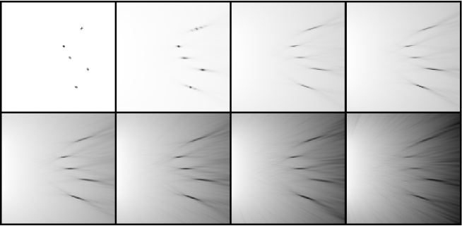
Figure 2: Numerical results for $\widetilde{H}(\omega)$ obtained by randomly selecting $J=M$ rows of the matrix $H(\omega)$, for different levels of noise: $SNR=\infty,80,40,20,10,5,2,1$ (from top left corner to bottom right corner).

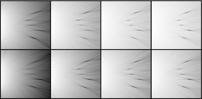
Figure 3: Numerical results for $\widetilde{H}(\omega)$ obtained by randomly selecting $J=M,2M,3M,4M$ rows of the matrix $H(\omega)$: first line $SNR=2$; second line $SNR=1$.

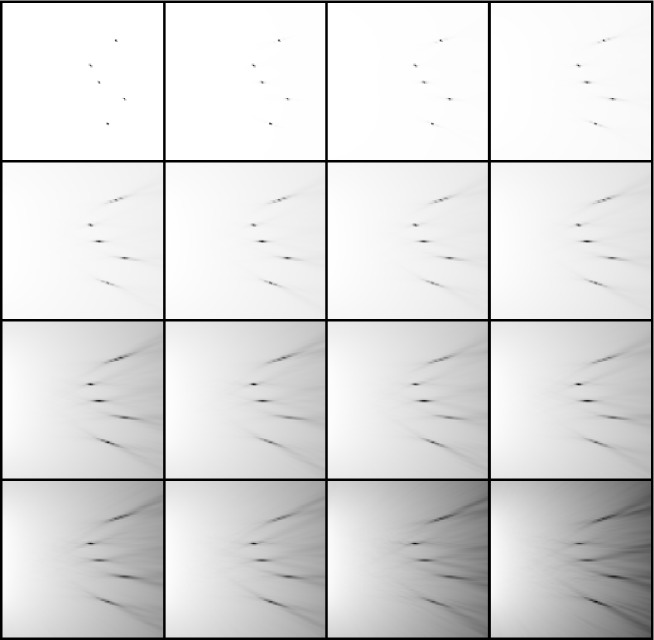
Figure 4: Numerical results obtained when the elements of the matrix $\widetilde{H}(\omega)$ are selected randomly as: $\widetilde{H}_{ij}(\omega)=H_{ij}(\omega)$ with probability $p$, and $\widetilde{H}_{ij}(\omega)=0$ with probability $1-p$. The lines correspond to the probability $p=1,0.5,0.25,0.1$, and the columns correspond to the noise level $SNR=\infty,10,5,2$.

References

- [1] L. Borcea, G. Papanicolaou, C. Tsogka, J. Berryman, Imaging and time reversal in random media, Inverse Problems, 18 (2002) 1247.
- [2] M. Fink, D. Cassereau, A. Derode, C. Prada, P. Roux, M. Tanter, J.-L. Thomas and F. Wu, Reports on Progress in Physics 63 (2000) 1933.
- [3] C. Prada, E. Kerbrat, D. Cassereau, M. Fink, Time reversal techniques in ultrasonic nondestructive testing of scattering media, Inverse Problems, 18 (2002) 1761.
- [4] C. Prada, L. Thomas, M. Fink, The Iterative Time Reversal Process: Analysis of the Convergence, Journal of the Acoustical Sociefy of America, 97 (1995) 62.
- [5] C. Prada, M. Fink, Eigenmodes of the time reversal operator: A solution to selective focusing in multiple-target media, Wave Motion, 20 (1994) 151.
- [6] C. Prada, S. Manneville. D. Spoliansky, M. Fink, Decomposition of the Time Reversal Operator: Detection and Selective Focusing on Two Scatterers, Journal of the Acoustical Society of America, 99 (1996) 2067.
- [7] F.K. Gruber, E.A. Marengo, A.J. Devaney, Timereversal imaging with multiple signal classification considering multiple scattering between the targets, Journal of the Acoustical Society of America, 115 (2004) 3042.
- [8] E.A. Marengo, F.K. Gruber, Subspace-Based Localization and Inverse Scattering of Multiply Scattering Point Targets, EURASIP Journal on Advances in Signal Processing, (2007) Article ID 17342.
- [9] H. Lev-Ari, A. J. Devaney, The time-reversal technique reinterpreted: Subspace-based signal processing for multi-static target location, IEEE Sensor Array and Multichannel Signal Processing Workshop, Cambridge (MA), USA, (2000) 509.
- [10] J. H. Taylor, Scattering Theory, Wiley, New York, 1972.
- [11] G. H.Golub, C. F. Van Loan, Matrix Computations, Johns Hopkins University Press, Baltimore, 1996.
- [12] A. Frieze, R. Kannan, S. Vempala, Fast Monte-Carlo algorithms for finding low rank approximations, Journal of the ACM, 51(6) (2004) 1025.
- [13] P. Drineas, R. Kannan, M. W. Mahoney, Fast Monte Carlo Algorithms for Matrices II: Computing a Low-Rank Approximation to a Matrix, SIAM Journal of Computing, 36(1) (2006) 158.
- [14] A. Deshpande, S. Vempala, Adaptive Sampling and Fast Low-rank Matrix Approximation, Proc. of 10th International Workshop on Randomization and Computation (RANDOM), 2006.
- [15] Dimitris Achlioptas, Frank McSherry, Fast computation of low-rank matrix approximations, Journal of the ACM, 54(2) (2007) Article 9.