Kadanoff-Baym approach to quantum transport through interacting nanoscale systems: From the transient to the steady-state regime

Abstract

We propose a time-dependent many-body approach to study the short-time dynamics of correlated electrons in quantum transport through nanoscale systems contacted to metallic leads. This approach is based on the time-propagation of the Kadanoff-Baym equations for the nonequilibrium many-body Green’s function of open and interacting systems out of equilibrium. An important feature of the method is that it takes full account of electronic correlations and embedding effects in the presence of time-dependent external fields, while at the same time satisfying the charge conservation law. The method further extends the Meir-Wingreen formula to the time domain for initially correlated states. We study the electron dynamics of a correlated quantum wire attached to two-dimensional leads exposed to a sudden switch-on of a bias voltage using conserving many-body approximations at Hartree-Fock, second Born and GW level. We obtain detailed results for the transient currents, dipole moments, spectral functions, charging times, and the many-body screening of the quantum wire as well as for the time-dependent density pattern in the leads, and we show how the time-dependence of these observables provides a wealth of information on the level structure of the quantum wire out of equilibrium. For moderate interaction strenghts the 2B and GW results are in excellent agreement at all times. We find that many-body effects beyond the Hartree-Fock approximation have a large effect on the qualitative behavior of the system and lead to a bias dependent gap closing and quasiparticle broadening, shortening of the transient times and washing out of the step features in the current-voltage curves.

I Introduction

The description of electron transport through nanoscale systems contacted to metallic leads is currently under intensive investigation especially due to the possibility of miniaturizing integrated devices in electrical circuits.book Several theoretical methods have been proposed to address the steady state properties of these systems.

Ab initio formulations based on Time-Dependent (TD) Density Functional Theoryrg.1984 ; vl.1999 ; sa.2004 ; sa2.2004 ; dvt.2004 ; ewk.2004 (DFT) and Current Density Functional Theoryvk.1996 ; v.2004 ; szvdv.2005 ; kbe.2006 ; jbg.2007 provide a virtual exact framework to account for correlation effects both in the leads and the device but lack of a systematic route to improve the level of the approximations. Ad hoc approximations have been successfully implemented to describe qualitative features of the I/V characteristic of molecular junctions in the Coulomb blockade regime.tfsb.2005 ; p.2005 ; se.2008 ; sgc.2008 More sophisticated approximations are, however, needed for, e.g., non-resonant tunneling transport through weakly coupled molecules.ewk.2004 ; dvpl.2000 ; stbmo.2003 ; qvclhn.2007 ; kby.2007

The possibility of including relevant physical processes through an insightful selection of Feynman diagrams is the main advantage of Many-Body Perturbation Theory (MBPT) over one-particle schemes. Even though computationally more expensive MBPT offers an invaluable tool to quantify the effects of electron correlations by analyzing, e.g., the quasi-particle spectra, life-times, screened interactions, etc. One of the most remarkable advances in the MBPT formulation of electron transport was given by Meir and Wingreen who provided an equation for the steady state current through a correlated device regionmw.1992 ; jwm.1994 thus generalizing the Landauer formula.l.1957 The Meir-Wingreen formula is cast in terms of the interacting Green’s function and self-energy in the device region and can be approximated using standard diagrammatic techniques. Exploiting Wick’s theoremFetterWalecka a general diagram for the self-energy can be written in terms of bare Green’s functions and interaction lines. Any approximation to the self-energy which contains a finite number of such diagrams does, however, violate many conservation laws. Conserving approximationsbk.1961 ; b.1962 ; vbdvls.2005 ; bbvl.2007 require the resummation of an infinite number of diagrams and are of paramount importance in nonequilibrium problems as they guarantee satisfaction of fundamental conservation laws such as charge conservation. Examples of conserving approximations are the Hartree-Fock (HF), second Born (2B), GW, T-matrix, and fluctuation exchange (FLEX) approximations.bs.1989 ; vlds.2006 The success of the GW approximationh.1965 ; ag.1998 in describing spectral features of atoms and moleculesnrdsdcf.2005 ; sdvl.2006 ; sdvl.2009 as well as of interacting model clustersvgh.1995 prompted efforts to implement the Meir-Wingreen formula at the GW level in simple molecular junctions and tight-binding models.tr.2007 ; dfmo.2007 ; wshm.2008 ; tr.2008 ; t.2008 ; shlm.2009

The advantage of using molecular devices in future nanoelectronics is, however, not only the miniaturization of integrated circuits. Nanodevices can work at the THertz regime and hence perform operations in few picoseconds or even faster. Space and time can both be considerably reduced. Nevertheless, at the sub-picosecond time scale stationary steady-state approaches are inadequate to extract crucial quantities like, e.g., the switching- or charging-time of a molecular diode, and consequently to understand how to optimize the device performance. Despite the importance that an increase in the operational speed may have in practical applications, the ultrafast dynamical response of nanoscale devices is still largely unexplored. This paper wants to make a further step towards the theoretical modeling of correlated TD quantum transport.

Recently several practical schemes have been proposed to tackle TD quantum transport problems of noninteracting electrons.ksarg.2005 ; zmjg.2005 ; hhlkch.2006 ; mgm.2007 ; bcg.2008 In some of these schemes the electron-electron interaction can be included within a TDDFT frameworksa.2004 ; ksarg.2005 and few calculations on the transient electron dynamics of molecular junctions have been performed at the level of the adiabatic local density approximation.cevt.2006 ; bsdv.2005 ; zwymc.2007 Alternatively, approaches based on Bohm trajectorieso.2007 ; aso.2009 or on the density matrix renormalization groupahfrbd.2006 have been put forward to calculate TD currents and densities through interacting quantum systems. So far, however, no one has extended the diagrammatic MBPT formulation of Meir and Wingreen to the time-domain. As in the steady-state case the MBPT formulation allows for including relevant scattering mechanisms via a proper selection of physically meaningful Feynman diagrams. The appealing nature of diagrammatic expansions renders MBPT an attractive alternative to investigate out-of-equilibrium systems.

In a recent Lettermssvl.2008 we proposed a time-dependent MBPT formulation of quantum transport which is based on the real-time propagation of the Kadanoff-Baym (KB) equationsdsvl.2006 ; dvl.2007 ; vfva.2009 ; bbvlds.2009 ; book2 ; d.1984 ; kb.2000 for open and interacting systems. The KB equations are equations of motion for the nonequilibrium Green’s function from which basic properties of the system can be calculated. It is the purpose of this paper to give a detailed account of the theoretical derivation and to extend the numerical analysis to quantum wires connected to two-dimensional leads. For practical calculations we have implemented the fully self-consistent HF, 2B and GW conserving approximations. Our results reduce to those of steady-state MBPT implementations in the long time limit. Having full access to the transient dynamics we are able, however, to extract novel information like the switching- and charging-times, the time-dependent renormalization of the electronic levels, the role of initial correlations, the time-dependent dipole moments etc. Furthermore, the non-locality in time of the 2B and GW self-energies allows us to highlight non-trivial memory effects occuring before the steady-state is reached. We also wish to emphasize that our approach is not limited to DC biases. Arbitrary driving fields like AC biases, voltage pulses, pumping fields, etc. can be dealt with at the same computational cost.

The paper is organized as follows. All derivations and formulas are given in Section II. We present the class of many-body systems that can be studied within our KB formulation in Section II.1 and derive the equations of motion for the nonequilibrium Green’s function in the device region in Section II.2 (see also Appendix A). The equations of motion are then used to prove the continuity equation for all conserving approximations, Section II.3, and to extend the Meir-Wingreen formula to the time domain for initially correlated systems, Section II.4. Using an inbedding technique in Section II.5 we derive the main equations to calculate the time-dependent density in the leads. In Section III we present the results of our TD simulations for a one-dimensional wire connected to two-dimensional leads. The Keldysh Green’s function, which is the basic quantity of the KB approach, of the open wire is studied in Section III.1 showing different time-dependent regimes relevant to the subsequent analysis. In Section III.2 and III.3 we calculate the TD current and dipole moment respectively. We find that the 2B and GW results are in excellent agreement at all times and can differ substantially from the HF results. We also perform the Fourier analysis of the transient oscillations and reveal the underlying out-of-equilibrium electronic structure of the open wire.skrg.2008 The dynamically screened interaction of the GW approximation is investigated in Section III.4 with emphasis on the time-scales of retardation effects. Section III.5 is devoted to the study of the TD rearrangement of the density in the two-dimensional leads after the switch-on of an external bias. Such an analysis permits us to test the validity of a commonly used assumption in quantum transport, i.e., that the leads remain in thermal equilibrium. Finally, in Section IV we draw our main conclusions and future perspectives.

II Theory

II.1 The model Hamiltonian

We consider a class of quantum correlated open systems (which we call central regions) coupled to noninteracting reservoirs (which we call leads), see Fig. 1.

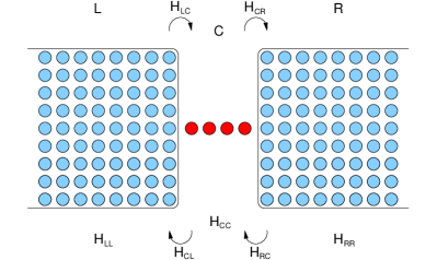
Figure 1: Sketch of the transport setup. The correlated central region (C) is coupled to semi-infinite left (L) and right (R) tight-binding leads via tunneling Hamiltonians $\mathbf{H}_{\alpha\textnormal{\scriptsize{C}}}$ and $\mathbf{H}_{\textnormal{\scriptsize{C}}\alpha}$, $\alpha={\rm L,R}$.

The Hamiltonian has the general form

$$\hat{H}(t)=\hat{H}_{\rm C}(t)+\sum_{\alpha}\hat{H}_{\alpha}(t)+\hat{H}_{T}-\mu\hat{N},$$ (1)

where $\hat{H}_{\rm C}$, $\hat{H}_{\alpha}$, $\hat{H}_{T}$ are the central region, the lead $\alpha$ and the tunneling Hamiltonians respectively and $\hat{N}$ is the particle number operator coupled to chemical potential $\mu$. We assume that there is no direct coupling between the leads. The correlated central region has a Hamiltonian of the form

$$\hat{H}_{\rm C}(t)=\sum_{ij,\sigma}h_{ij}(t)\hat{d}_{i\sigma}^{\dagger}\hat{d}_{j\sigma}+\frac{1}{2}\sum_{\begin{subarray}{c}ijkl\\ \sigma\sigma^{\prime}\end{subarray}}v_{ijkl}\hat{d}_{i\sigma}^{\dagger}\hat{d}_{j\sigma^{\prime}}^{\dagger}\hat{d}_{k\sigma^{\prime}}\hat{d}_{l\sigma},$$ (2)

where $i,j$ label a complete set of one-particle states in the central region, $\sigma,\sigma^{\prime}$ are spin-indices and $\hat{d}^{\dagger},\hat{d}$ are the creation and annihilation operators respectively. The one-body part of the Hamiltonian $h_{ij}(t)$ may have an arbitrary time-dependence, describing, e.g., a gate voltage or pumping fields. The two-body part accounts for interactions between the electrons where $v_{ijkl}$ are, for example in the case of a molecule, the standard two-electron integrals of the Coulomb interaction. The lead Hamiltonians have the form

$$\hat{H}_{\alpha}(t)=U_{\alpha}(t)\hat{N}_{\alpha}+\sum_{ij,\sigma}h_{ij}^{\alpha}\,\hat{c}_{i\sigma\alpha}^{\dagger}\hat{c}_{j\sigma\alpha},$$ (3)

where the creation and annihilation operators for the leads are denoted by $\hat{c}^{\dagger}$ and $\hat{c}$. Here $\hat{N}_{\alpha}=\sum_{i,\sigma}\hat{c}_{i\sigma\alpha}^{\dagger}\hat{c}_{i\sigma\alpha}$ is the operator describing the number of particles in lead $\alpha$. The one-body part of the Hamiltonian $h_{ij}^{\alpha}$ describes metallic leads and can be calculated using a tight-binding representation, or a real-space grid or any other convenient basis set. We are interested in exposing the leads to an external electric field which varies on a time-scale much longer than the typical plasmon time-scale. Then, the coarse-grained time evolution can be performed assuming a perfect instantaneous screening in the leads and the homogeneous time-dependent field $U_{\alpha}(t)$ can be interpreted as the sum of the external and the screening field, i.e., the applied bias. This effectively means that the leads are treated at a Hartree mean field level. We finally consider the tunneling Hamiltonian $\hat{H}_{T}$

$$\hat{H}_{T}=\sum_{ij,\sigma\alpha}V_{i,j\alpha}[\hat{d}_{i\sigma}^{\dagger}\hat{c}_{j\sigma\alpha}+\hat{c}_{j\sigma\alpha}^{\dagger}\hat{d}_{i\sigma}]$$ (4)

which describes the coupling of the leads to the interacting central region. This completes the full description of the Hamiltonian of the system. In the next section we study the equations of motion for the corresponding Green’s function.

II.2 Equation of motion for the Keldysh Green’s function

We assume the system to be contacted and in equilibrium at inverse temperature $\beta$ before time $t=t_{0}$ and described by Hamiltonian $\hat{H}_{0}$. For times $t>t_{0}$ the system is driven out of equilibrium by an external bias and we aim to study the time-evolution of the electron density, current, etc.. In order to describe the electron dynamics in this system we use Keldysh Green’s function theory (for a review see Ref.d.1984, ) which allows us to include many-body effects in a diagrammatic way. The Keldysh Green’s function is defined as the expectation value of the contour-ordered product

$$\mbox{\boldmath$\mathcal{G}$}_{rs}(z,z^{\prime}) = -i\frac{{\rm Tr}\left\{\mathcal{T}[e^{-i\int d\bar{z}\hat{H}(\bar{z})}\hat{a}_{r}(z)\hat{a}^{\dagger}_{s}(z^{\prime})]\right\}}{{\rm Tr}\left\{e^{-\beta\hat{H}_{0}}\right\}}$$ (5)

$$= -i\langle\mathcal{T}[\hat{a}_{r}(z)\hat{a}^{\dagger}_{s}(z^{\prime})]\rangle,$$

where $\hat{a}$ and $\hat{a}^{\dagger}$ are either lead or central region operators and the indices $r$ and $s$ are collective indices for position and spin. The variable $z$ is a time contour variable that specifies the location of the operators on the time contour. The operator $\mathcal{T}$ orders the operators along the Keldysh contour displayed in Fig. 2, consisting of two real time branches and the imaginary track running from $t_{0}$ to $t_{0}-i\beta$. In the definition of the Green’s function the trace is taken with respect to the many-body states of the system.
All time-dependent one-particle properties can be calculated from $\mathcal{G}$. For instance, the time-dependent density matrix is given as

$$n_{rs}(t)=-i\mbox{\boldmath$\mathcal{G}$}_{rs}(t_{-},t_{+}),$$ (6)

where the times $t_{\pm}$ lie on the lower/upper branch of the contour. The equations of motion for the Green’s function of the full system can be easily derived from the definition Eq. (5) and read

$$i\partial_{z}\mbox{\boldmath$\mathcal{G}$}(z,z^{\prime}) = \delta(z,z^{\prime})\mathbf{1}+\mathbf{H}(z)\mbox{\boldmath$\mathcal{G}$}(z,z^{\prime})$$ (7)

$$+ \int d\bar{z}\,\mbox{\boldmath$\Sigma$}^{\rm MB}(z,\bar{z})\mbox{\boldmath$\mathcal{G}$}(\bar{z},z^{\prime}),$$

$$-i\partial_{z^{\prime}}\mbox{\boldmath$\mathcal{G}$}(z,z^{\prime}) = \delta(z,z^{\prime})\mathbf{1}+\mbox{\boldmath$\mathcal{G}$}(z,z^{\prime})\mathbf{H}(z^{\prime})$$ (8)

$$+ \int d\bar{z}\,\mbox{\boldmath$\mathcal{G}$}(z,\bar{z})\mbox{\boldmath$\Sigma$}^{\rm{MB}}(\bar{z},z),$$

where $\mbox{\boldmath$\Sigma$}^{\rm MB}$ is the many-body self-energy, $\mathbf{H}(z)$ is the matrix representation of the one-body part of the full Hamiltonian and the integration is performed over the Keldysh-contour. This equation of motion needs to be solved with the boundary conditionsk.1957 ; ms.1959

$$\begin{split}\mbox{\boldmath$\mathcal{G}$}(t_{0},z^{\prime})&=-\mbox{\boldmath$\mathcal{G}$}(t_{0}-i\beta,z^{\prime}),\\ \mbox{\boldmath$\mathcal{G}$}(z,t_{0})&=-\mbox{\boldmath$\mathcal{G}$}(z,t_{0}-i\beta),\end{split}$$ (9)

which follow directly from the definition of the Green’s function Eq. (5). Explicitly, the one-body Hamiltonian $\mathbf{H}$ for the case of two leads, Left (L) and Right (R) connected to a central region (C), is

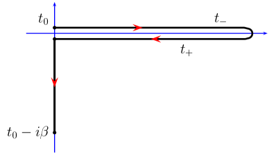
Figure 2: Keldysh contour $\gamma$. Times on the upper/lower branch are specified with the subscript $\mp$.

$$\mathbf{H}=\left[\begin{array}[]{ccc}\mathbf{H}_{\textnormal{\scriptsize{LL}}}&\mathbf{H}_{\textnormal{\scriptsize{LC}}}&\mathbf{0}\\ \mathbf{H}_{\textnormal{\scriptsize{CL}}}&\mathbf{H}_{\textnormal{\scriptsize{CC}}}&\mathbf{H}_{\textnormal{\scriptsize{CR}}}\\ \mathbf{0}&\mathbf{H}_{\textnormal{\scriptsize{RC}}}&\mathbf{H}_{\textnormal{\scriptsize{RR}}}\end{array}\right]$$ (10)

where the different block matrices describe the projections of the one-body part $\mathbf{H}$ of the Hamiltonian onto different subregions. They are explicitly given as

$$\left(\mathbf{H}_{\alpha\alpha}\right)_{i\sigma,j\sigma^{\prime}}(z) = \left[h_{ij}^{\alpha}+\delta_{ij}(U_{\alpha}(z)-\mu)\right]\delta_{\sigma\sigma^{\prime}},$$ (11)

$$\left(\mathbf{H}_{\rm{CC}}\right)_{i\sigma,j\sigma^{\prime}}(z) = \left[h_{ij}(z)-\delta_{ij}\mu\right]\delta_{\sigma\sigma^{\prime}},$$ (12)

$$\left(\mathbf{H}_{\rm{C}\alpha}\right)_{i\sigma,j\sigma^{\prime}} = \left(\mathbf{H}_{\alpha\rm{C}}^{\dagger}\right)_{j\sigma^{\prime},i\sigma,}=V_{i,j\alpha}\delta_{\sigma\sigma^{\prime}}.$$ (13)

We focus on the dynamical processes occuring in the central region. These are described by the Green’s function $\mbox{\boldmath$\mathcal{G}$}_{\rm{CC}}$ projected onto region C. We therefore want to extract from the block matrix structure for the Green’s function

$$\mbox{\boldmath$\mathcal{G}$}=\left[\begin{array}[]{ccc}\mbox{\boldmath$\mathcal{G}$}_{\textnormal{\scriptsize{LL}}}&\mbox{\boldmath$\mathcal{G}$}_{\textnormal{\scriptsize{LC}}}&\mbox{\boldmath$\mathcal{G}$}_{\textnormal{\scriptsize{LR}}}\\ \mbox{\boldmath$\mathcal{G}$}_{\textnormal{\scriptsize{CL}}}&\mbox{\boldmath$\mathcal{G}$}_{\textnormal{\scriptsize{CC}}}&\mbox{\boldmath$\mathcal{G}$}_{\textnormal{\scriptsize{CR}}}\\ \mbox{\boldmath$\mathcal{G}$}_{\textnormal{\scriptsize{RL}}}&\mbox{\boldmath$\mathcal{G}$}_{\textnormal{\scriptsize{RC}}}&\mbox{\boldmath$\mathcal{G}$}_{\textnormal{\scriptsize{RR}}}\end{array}\right]$$ (14)

an equation for $\mbox{\boldmath$\mathcal{G}$}_{\rm{CC}}$. The many-body self-energy in Eq. (7) has nonvanishing entries only for indices in region C. This is an immediate consequence of the fact that the diagrammatic expansion of the self-energy starts and ends with and interaction line which in our case is confined in the central region (see last term of Eq. (2)). This also implies that $\mbox{\boldmath$\Sigma$}^{\rm{MB}}[\mbox{\boldmath$\mathcal{G}$}_{\rm{CC}}]$ is a functional of $\mbox{\boldmath$\mathcal{G}$}_{\rm{CC}}$ only. From these considerations it follows that in the one-particle basis the matrix structure of $\mbox{\boldmath$\Sigma$}^{\rm{MB}}$ is given as

$$\mbox{\boldmath$\Sigma$}^{\rm{MB}}=\left[\begin{array}[]{ccc}0&0&0\\ 0&\mbox{\boldmath$\Sigma$}^{\rm{MB}}_{\rm{CC}}[\mbox{\boldmath$\mathcal{G}$}_{\rm{CC}}]&0\\ 0&0&0\end{array}\right].$$ (15)

The projection of the equation of motion (7) onto regions ${\rm CC}$ and $\alpha{\rm C}$ yields

$$\begin{split}&\Bigl{\{}i\partial_{z}\mathbf{1}-\mathbf{H}_{\rm CC}(z)\Bigr{\}}\mbox{\boldmath$\mathcal{G}$}_{\rm CC}(z,z^{\prime})=\delta(z,z^{\prime})\mathbf{1}\,\,+\\ &\sum_{\alpha}\mathbf{H}_{{\rm C}\alpha}\mbox{\boldmath$\mathcal{G}$}_{\alpha\rm C}(z,z^{\prime})+\int d\bar{z}\,\mbox{\boldmath$\Sigma$}_{\rm CC}^{\rm MB}(z,\bar{z})\mbox{\boldmath$\mathcal{G}$}_{\rm CC}(\bar{z},z^{\prime})\end{split}$$ (16)

for the central region and

$$\Bigl{\{}i\partial_{z}\mathbf{1}-\mathbf{H}_{\alpha\alpha}(z)\Bigr{\}}\mbox{\boldmath$\mathcal{G}$}_{\alpha\rm{C}}(z,z^{\prime})=\mathbf{H}_{\alpha\rm{C}}\mbox{\boldmath$\mathcal{G}$}_{\rm{CC}}(z,z^{\prime})$$ (17)

for the projection on $\alpha{\rm C}$. The latter equation can be solved for $\mbox{\boldmath$\mathcal{G}$}_{\alpha\rm{C}}$, taking into account the boundary conditions of Eq. (9), to yield

$$\begin{split}\mbox{\boldmath$\mathcal{G}$}_{\alpha\rm C}(z,z^{\prime})=\int d\bar{z}\,\mathbf{g}_{\alpha\alpha}(z,\bar{z})\,\mathbf{H}_{\alpha\rm C}\mbox{\boldmath$\mathcal{G}$}_{\rm CC}(\bar{z},z^{\prime}),\end{split}$$ (18)

where the integral is along the Keldysh contour. Here we defined $\mbox{\boldmath$g$}_{\alpha\alpha}$ as the solution of

$$\Bigl{\{}i\partial_{z}\mathbf{1}-\mathbf{H}_{\alpha\alpha}(z)\Bigr{\}}\mbox{\boldmath$g$}_{\alpha\alpha}(z,z^{\prime})=\delta(z,z^{\prime})\mathbf{1},$$ (19)

with boundary conditions Eq. (9). The function $\mbox{\boldmath$g$}_{\alpha\alpha}$ is the Green’s function of the isolated and biased $\alpha$-lead. We wish to stress that a Green’s function $\mbox{\boldmath$g$}_{\alpha\alpha}$ with boundary conditions Eq. (9) automatically ensures the correct boundary conditions for the $\mbox{\boldmath$\mathcal{G}$}_{\alpha\rm C}(z,z^{\prime})$ in Eq. (18). Any other boundary conditions would not only lead to an unphysical transient behavior but also to different steady state results.sa.2004 This is the case for, e.g., initially uncontacted Hamiltonians in which the equilibrium chemical potential of the leads is replaced by the electrochemical potential, i.e., the sum of the chemical potential and the bias.

Taking into account Eq. (18) the first term on the righthand side of Eq. (16) becomes

$$\sum_{\alpha}\mathbf{H}_{\rm{C}\alpha}\mbox{\boldmath$\mathcal{G}$}_{\alpha\rm{C}}(z,z^{\prime})=\int d\bar{z}\,\mbox{\boldmath$\Sigma$}_{\rm{em}}(z,\bar{z})\mbox{\boldmath$\mathcal{G}$}_{\rm{CC}}(\bar{z},z^{\prime}),$$ (20)

where we have introduced the embedding self-energy

$$\mbox{\boldmath$\Sigma$}_{\rm{em}}(z,z^{\prime})=\sum_{\alpha}\mbox{\boldmath$\Sigma$}_{\rm{em},\alpha}(z,z^{\prime})=\sum_{\alpha}\mathbf{H}_{{\rm C}\alpha}\,\mathbf{g}_{\alpha\alpha}(z,z^{\prime})\mathbf{H}_{\alpha\rm C},$$ (21)

which accounts for the tunneling of electrons from the central region to the leads and vice versa. The embedding self-energies $\mbox{\boldmath$\Sigma$}_{\rm{em},\alpha}$ are independent of the electronic interactions and hence of $\mbox{\boldmath$\mathcal{G}$}_{\rm{CC}}$, and are therefore completely known once the lead Hamiltonians $\hat{H}_{\alpha}$ of Eq. (3) are specified. Inserting (20) back to (16) then gives the equation of motion

$$\begin{split}&\Bigl{\{}i\partial_{z}\mathbf{1}-\mathbf{H}_{\rm CC}(z)\Bigr{\}}\mbox{\boldmath$\mathcal{G}$}_{\rm CC}(z,z^{\prime})\\ &=\delta(z,z^{\prime})\mathbf{1}+\int d\bar{z}\,\left[\mbox{\boldmath$\Sigma$}_{\rm CC}^{\rm MB}+\mbox{\boldmath$\Sigma$}_{\rm em}\right](z,\bar{z})\,\mbox{\boldmath$\mathcal{G}$}_{\rm CC}(\bar{z},z^{\prime}).\end{split}$$ (22)

An adjoint equation can similarly be derived from Eq. (8). Equation (22) is an exact equation for the Green’s function $\mbox{\boldmath$\mathcal{G}$}_{\rm{CC}}$, for the class of Hamiltonians of Eq. (1), provided that an exact expression for $\mbox{\boldmath$\Sigma$}^{\rm{MB}}_{\rm CC}[\mbox{\boldmath$\mathcal{G}$}_{\rm{CC}}]$ as a functional of $\mbox{\boldmath$\mathcal{G}$}_{\rm{CC}}$ is inserted. In practical implementations Eq. (22) is converted to a set of coupled real-time equations, known as the Kadanoff-Baym equations (see Appendix A). These equations are solved by means of time-propagation techniques.sdvl.2009b For the case of unperturbed systems the contributions of the integral in Eq. (22) coming from the real-time branches of the contour cancel and the integral needs only to be taken on the imaginary vertical track. The equation for the Green’s function then becomes equivalent to the one of the equilibrium finite-temperature formalism. In a time-dependent situation the vertical track therefore accounts for initial correlations due to both many-body interactions, incorporated in $\mbox{\boldmath$\Sigma$}^{\rm{MB}}_{\rm CC}$, and contacts with the leads, incorporated in $\mbox{\boldmath$\Sigma$}_{\rm{em}}$. In our implementation (see Appendix A) we always solve the contacted and correlated equation first on the the imaginary track, before we propagate the Green’s function in time in the presence of an external field. However, to study initial correlations we are free to set the embedding and many-body self-energy to zero before time-propagation, which is equivalent to neglect the vertical track of the contour.mssvl.2008 This would correspond to starting with an equilibrium configuration that describes an initially uncontacted and noninteracting central region. This class of initial configurations is commonly used in quantum transport calculations, where both the interactions and the couplings are considered to be switched on in the distant past. The assumption is then made that the system thermalizes before the bias is switched on. Even when this assumption is fulfilled there are practical difficulties to study transient phenomena, as one has to propagate the system until it has thermalized before a bias can be switched on. It is therefore an advantage of our approach that thermalization assumptions are not necessary.
To solve the equation of motion Eq. (22) we need to find an approximation for the many-body self-energy $\mbox{\boldmath$\Sigma$}^{\rm{MB}}[\mbox{\boldmath$\mathcal{G}$}_{\rm{CC}}]$ as a functional of the Green’s function $\mbox{\boldmath$\mathcal{G}$}_{\rm{CC}}$. This approximation can be constructed using diagrammatic techniques based on Wick’s theorem familiar from equilibrium theory FetterWalecka which can be straightforwardly be extended to the case of contour-ordered Green’s functions.d.1984 In our case the perturbative expansion is in powers of the two-body interaction and the unperturbed system consists of the noninteracting, but contacted and biased system. We stress, however, that eventually all our expressions are given in terms of fully dressed Green’s functions leading to fully self-consistent equations for the Green’s function. This full self-consistency is essential to guarantee the satisfaction of the charge conservation law, as is discussed in the next section.

II.3 Charge conservation

The approximations for $\mbox{\boldmath$\Sigma$}^{\rm{MB}}_{\rm CC}[\mbox{\boldmath$\mathcal{G}$}_{\rm{CC}}]$ that we use in this work involve the Hartree-Fock, second Born and GW approximation, which are discussed in detail in Refs. dvl.2007, ; sdvl.2009, ; sdvl.2009b, ; dvl.2005, and are displayed pictorially in Fig. 3.

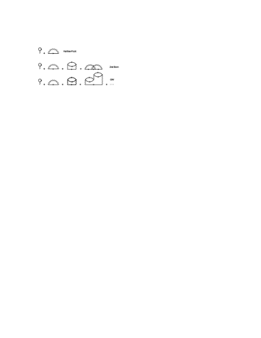
Figure 3: Diagrammatic representation of the many-body approximations for $\mbox{\boldmath$\Sigma$}_{\rm CC}^{\rm MB}$.

These are all examples of so-called conserving approximations for the self-energy, that guarantee satisfaction of fundamental conservation laws such as charge conservation. As shown by Baym b.1962 , a self-energy approximation is conserving whenever it can be written as the derivative of a functional $\Phi$, i.e.

$$\mbox{\boldmath$\Sigma$}^{\rm{MB}}_{{\rm CC},rs}[\mbox{\boldmath$\mathcal{G}$}_{\rm{CC}}](z,z^{\prime})=\frac{\delta\Phi[\mbox{\boldmath$\mathcal{G}$}_{\rm{CC}}]}{\delta\mbox{\boldmath$\mathcal{G}$}_{{\rm CC},sr}(z^{\prime},z)}.$$ (23)

This form of the self-energy is by itself not sufficient to guarantee that the conservation laws are obeyed. A second condition is that the equations of motion for the Green’s function need to be solved fully self-consistently for this form of the self-energy (see, e.g., Ref. sdvl.2009, ). For an open system, like our central region, charge conservation does not imply that the time derivative of the number of particles $N_{\rm{C}}(t)$ is constant in time. It rather implies that the time-derivative of $N_{\rm{C}}(t)$, also known as the displacement current, is equal to the sum of the currents that flow into the leads. Below we give a proof in which the importance of the $\Phi$-derivability is clarified. We start by writing the number of particles $N_{\rm{C}}(t)$ as (see Eq. (6))

$$N_{\rm C}(t)=-i{\rm Tr}_{\rm C}\left[\mbox{\boldmath$\mathcal{G}$}_{\rm CC}(t_{-},t_{+})\right],$$ (24)

where the trace is taken over all one-particle indices in the central region. Subtracting the equation of motion (22) from its adjoint and setting $z=t_{-},z^{\prime}=t_{+}$ then yields

$$\frac{dN_{\rm C}(t)}{dt}=-2{\rm Re}\,{\rm Tr}_{\rm C}\left[\int d\bar{z}\,\mbox{\boldmath$\Sigma$}_{\rm{CC}}(t_{-},\bar{z})\mbox{\boldmath$\mathcal{G}$}_{\rm{CC}}(\bar{z},t_{+})\right],$$ (25)

where $\mbox{\boldmath$\Sigma$}_{\rm{CC}}=\mbox{\boldmath$\Sigma$}_{\rm{CC}}^{\rm{MB}}+\mbox{\boldmath$\Sigma$}_{\rm{em}}$. By similar reasonings we can calculate the current $I_{\alpha}$ flowing across the interface between lead $\alpha$ and the central region. The total number of particles in lead $\alpha$ is $N_{\alpha}=-i{\rm Tr}_{\alpha}\left[\mbox{\boldmath$\mathcal{G}$}_{\alpha\alpha}(t_{-},t_{+})\right]$, where the trace is taken over all one-particle indices in lead $\alpha$. Projecting the equation of motion (7) on region $\alpha\alpha$ yields

$$i\partial_{z}\mbox{\boldmath$\mathcal{G}$}_{\alpha\alpha}(z,z^{\prime}) = \delta(z,z^{\prime})\mathbf{1}+\mathbf{H}_{\alpha\alpha}(z)\mbox{\boldmath$\mathcal{G}$}_{\alpha\alpha}(z,z^{\prime})$$ (26)

$$+ \mathbf{H}_{\alpha\rm C}(z)\mbox{\boldmath$\mathcal{G}$}_{{\rm C}\alpha}(z,z^{\prime}).$$

Subtracting this equation from its adjoint one finds

$$I_{\alpha}(t) = -\frac{dN_{\alpha}(t)}{dt}=2{\rm Re}\,{\rm Tr}_{\alpha}\left[\mathbf{H}_{\alpha\rm C}\mbox{\boldmath$\mathcal{G}$}_{{\rm C}\alpha}(t_{-},t_{+})\right]$$ (27)

$$= 2{\rm Re}\,{\rm Tr}_{\rm C}\left[\mbox{\boldmath$\mathcal{G}$}_{{\rm C}\alpha}(t_{-},t_{+})\mathbf{H}_{\alpha\rm C}\right].$$

Substituting in this expression the explicit solution (18) for $\mbox{\boldmath$\mathcal{G}$}_{\alpha\rm C}$ as well as the solution for its adjoint $\mbox{\boldmath$\mathcal{G}$}_{{\rm C}\alpha}$ we can write the current $I_{\alpha}$ in terms of the embedding self-energy $\mbox{\boldmath$\Sigma$}_{\rm{em},\alpha}$ as

$$I_{\alpha}(t)=2{\rm Re}\,{\rm Tr}_{\rm C}\left[\int d\bar{z}\,\mbox{\boldmath$\mathcal{G}$}_{\rm CC}(t_{-},\bar{z})\mbox{\boldmath$\Sigma$}_{{\rm em},\alpha}(\bar{z},t_{+})\right].$$ (28)

Exploiting this result Eq. (25) takes the form

$$\begin{split}&\frac{dN_{\rm C}(t)}{dt}=I_{\rm L}+I_{\rm R}-\int d\bar{z}\,{\rm Tr}_{\rm C}\\ &\times\left[\mbox{\boldmath$\Sigma$}^{\rm MB}_{\rm{CC}}(t_{-},\bar{z})\mbox{\boldmath$\mathcal{G}$}_{\rm{CC}}(\bar{z},t_{+})-\mbox{\boldmath$\mathcal{G}$}_{\rm{CC}}(t_{-},\bar{z})\mbox{\boldmath$\Sigma$}^{\rm MB}_{\rm{CC}}(\bar{z},t_{+})\right].\end{split}$$ (29)

Charge conservation implies that the integral in Eq. (29) vanishes. This is a direct consequence of the invariance of the functional $\Phi$ under gauge transformations. Indeed, changing the external potential by an arbitrary purely time-dependent function $\Lambda_{r}(z)$ (with the boundary condition $\Lambda_{r}(t_{0})=\Lambda_{r}(t_{0}-i\beta))$ changes the Green’s function according tob.1962

$$\mbox{\boldmath$\mathcal{G}$}_{{\rm CC},rs}[\Lambda](z,z^{\prime})=e^{i\Lambda_{r}(z)}\mbox{\boldmath$\mathcal{G}$}_{{\rm CC},rs}(z,z^{\prime})e^{-i\Lambda_{s}(z^{\prime})},$$ (30)

as can be checked directly from the equations of motion for the Green’s function. From its definition Eq. (23) it follows that the $\Phi$-functional consists of closed diagrams in terms of the Green’s function $\mbox{\boldmath$\mathcal{G}$}_{\rm CC}$. The phase factors of Eq. (30) thus cancel each other at every vertex and therefore $\Phi$ is independent of the functions $\Lambda_{r}$. This implies that

$$0 = \sum_{q\in\rm C}\frac{\delta\Phi}{\delta\Lambda_{q}(z)}$$ (31)

$$= \sum_{qrs\in\rm C}\int d\bar{z}d\bar{z}^{\prime}\frac{\delta\Phi}{\delta\mbox{\boldmath$\mathcal{G}$}_{{\rm CC},sr}(\bar{z}^{\prime},\bar{z})}\frac{\delta\mbox{\boldmath$\mathcal{G}$}_{{\rm CC},sr}(\bar{z}^{\prime},\bar{z})}{\delta\Lambda_{q}(z)}$$

$$= \sum_{qrs\in\rm C}\int d\bar{z}d\bar{z}^{\prime}\,\mbox{\boldmath$\Sigma$}_{{\rm CC},rs}^{\rm MB}(\bar{z},\bar{z}^{\prime})\frac{\delta\mbox{\boldmath$\mathcal{G}$}_{{\rm CC},sr}(\bar{z}^{\prime},\bar{z})}{\delta\Lambda_{q}(z)},$$

where the sums run over all one-particle indices in the central region. Here we explicitly used the $\Phi$-derivability condition of the self-energy of Eq. (23). If we now insert the derivative of the Green’s function with respect to $\Lambda_{r}$ from Eq. (30) in Eq. (31) and evaluate the resulting expression in $z=t_{\pm}$ we obtain the integral in Eq. (29). Therefore the last term in Eq. (29) vanishes and the time-derivative of the number of particles $N_{\rm C}(t)$ in the central region is equal to the sum of the currents that flow into the leads. We mention that in the long time limit the number of particles in region C is constant provided that the system attains a steady state. In this case $I_{\rm L}+I_{\rm R}=0$ and we recover the result of Ref. tr.2008, as a special case.

II.4 Equation for the time-dependent current

The time-dependent current in Eq. (28) accounts for the initial many-body and embedding effects. In the absence of an external perturbation $I_{\alpha}(t)=0$ at any time. The exact vanishing of the current is guaranteed by the contribution of the vertical track in the integral. Discarding this contribution is equivalent to starting with an initially uncorrelated and uncontacted system in which case there will be some thermalization time during which charge fluctuations will give rise to nonzero transient currents.
Equation (28) involves an integral over the Keldysh contour. Using the extended Langreth theoreml.book ; sa.2004 ; TDDFTbook for the contour of Fig. 2 we can express $I_{\alpha}(t)$ in terms of real time and imaginary time integrals

$$I_{\alpha}(t)=2\textnormal{Re}\,{\rm Tr}_{\rm C}\left[\int_{t_{0}}^{t}d\bar{t}\,\mbox{\boldmath$\mathcal{G}$}_{\rm CC}^{<}(t,\bar{t})\mbox{\boldmath$\Sigma$}_{{\rm em},\alpha}^{A}(\bar{t},t)\right.$$

$$+\int_{t_{0}}^{t}d\bar{t}\,\mbox{\boldmath$\mathcal{G}$}_{\rm CC}^{R}(t,\bar{t})\mbox{\boldmath$\Sigma$}_{{\rm em},\alpha}^{<}(\bar{t},t)$$

$$\left.-i\int_{0}^{\beta}d\tau\,\mbox{\boldmath$\mathcal{G}$}_{\rm CC}^{\rceil}(t,\tau)\mbox{\boldmath$\Sigma$}_{{\rm em},\alpha}^{\lceil}(\tau,t)\right],$$ (32)

where we refer to Appendix A for the definition of the various superscripts. Equation (32) provides a generalization of the Meir-Wingreen formulamw.1992 to the transient time-domain. As anticipated the last term in Eq. (32) explicitly accounts for the effects of initial correlations and initial-state dependence. If one assumes that both dependences are washed out in the long-time limit ($t\rightarrow\infty$), then the last term in Eq. (32) vanishes and we can safely take the limit $t_{0}\rightarrow-\infty$. Furthermore, if in this limit the Green’s function becomes a a function of the relative times only, i.e., $\mbox{\boldmath$\mathcal{G}$}_{\rm CC}(t,t^{\prime})\rightarrow\mbox{\boldmath$\mathcal{G}$}_{\rm CC}(t-t^{\prime})$, we can Fourier transform with respect to the relative time to obtain the Green’s function $\mbox{\boldmath$\mathcal{G}$}_{\rm CC}(\omega)$ and the self-energy $\mbox{\boldmath$\Sigma$}_{\rm{em}}(\omega)$ in frequency or energy space. This is typically the case for DC bias voltages where $\lim_{t\rightarrow\infty}U_{\alpha}(t)=U_{\alpha}$. In terms of the Fourier transformed quantities Eq. (32) reduces to the Meir-Wingreen formulamw.1992 for the steady state current

$$I_{\alpha}^{S}=-i\,{\rm Tr}_{\rm C}\int_{-\infty}^{\infty}\frac{d\omega}{2\pi}\mbox{\boldmath$\Gamma$}_{\alpha}(\omega)\Bigl{\{}\mbox{\boldmath$\mathcal{G}$}_{\rm CC}^{<}(\omega)-2i\pi f_{\alpha}(\omega){\bf A}(\omega)\Bigr{\}},$$ (33)

where

$$\mbox{\boldmath$\Gamma$}_{\alpha}(\omega)=-2\,{\rm Im}\,\{\mbox{\boldmath$\Sigma$}_{\rm{em},\alpha}^{R}(\omega)\},$$ (34)

$${\bf A}(\omega)=-\frac{1}{2\pi i}[\mbox{\boldmath$\mathcal{G}$}_{\rm CC}^{R}(\omega)-\mbox{\boldmath$\mathcal{G}$}_{\rm CC}^{A}(\omega)],$$ (35)

and where $f_{\alpha}$ is the Fermi distribution for lead $\alpha$ with electrochemical potential $\mu+U_{\alpha}$. This expression has been used recently to perform steady state transport calculations at GW level.tr.2007 ; tr.2008 ; t.2008 The present formalism allows for an extension of this work to the time-dependent regime.

II.5 Electron density in the leads

In our investigations we are not only interested in calculating the density in the central region, but are also interested in studying the densities in the leads. In the following we will therefore derive an equation from which these lead densities can be calculated. If we on the righthand side of Eq. (26) insert the adjoint of Eq. (18) we obtain the expression

$$i\partial_{z}\mbox{\boldmath$\mathcal{G}$}_{\alpha\alpha}(z,z^{\prime}) = \delta(z,z^{\prime})\mathbf{1}+\mathbf{H}_{\alpha\alpha}(z)\mbox{\boldmath$\mathcal{G}$}_{\alpha\alpha}(z,z^{\prime})$$ (36)

$$+ \int d\bar{z}\mbox{\boldmath$\Sigma$}_{\rm{in},\alpha}(z,\bar{z})\mbox{\boldmath$g$}_{\alpha\alpha}(\bar{z},z^{\prime}),$$

where we defined the inbedding self-energy as

$$\mbox{\boldmath$\Sigma$}_{\rm{in},\alpha}(z,z^{\prime})=\mathbf{H}_{\alpha{\rm C}}\mbox{\boldmath$\mathcal{G}$}_{\rm{CC}}(z,z^{\prime})\mathbf{H}_{{\rm C}\alpha}.$$ (37)

If we solve Eq. (36) in terms of $\mbox{\boldmath$g$}_{\alpha\alpha}$ and take the time arguments at $t_{\pm}$ we obtain

$$\mbox{\boldmath$\mathcal{G}$}_{\alpha\alpha}(t_{-},t_{+}) = \mbox{\boldmath$g$}_{\alpha\alpha}(t_{-},t_{+})+$$

$$+ \int d\bar{z}d\bar{\bar{z}}\mbox{\boldmath$g$}_{\alpha\alpha}(t_{-},\bar{z})\mbox{\boldmath$\Sigma$}_{\rm{in},\alpha}(\bar{z},\bar{\bar{z}})\mbox{\boldmath$g$}_{\alpha\alpha}(\bar{\bar{z}},t_{+}).$$

We see from Eq. (6) that with this equation we can obtain the spin occupation of orbital $i$ in lead $\alpha$ by taking $r=s=i\sigma\alpha$. The integral in Eq. (LABEL:leaddens) is taken along the Keldysh contour. In practice we solve the Kadanoff-Baym equations for $\mbox{\boldmath$\mathcal{G}$}_{\rm{CC}}$ first. After this we construct the inbedding self-energy $\mbox{\boldmath$\Sigma$}_{\rm{in}}$ and calculate the lead density from Eq. (LABEL:leaddens) converted into real time, using the conversion table of Ref. TDDFTbook, .

III Numerical results

In this Section we specialize to central regions consisting of quantum chains modelled using a tight-binding parametrization. We studied the case for which the chain extends from site 1 to site 4 and is coupled to a left and right two-dimensional reservoirs with 9 transverse channels in the left and right leads, as illustrated in Fig. 1. The parameters for the system are chosen as follows. The longitudinal and transverse nearest neighbor hoppings in the leads are set to $T_{\alpha}^{\lambda}=T_{\alpha}^{\tau}=-2.0$, $\alpha={\rm L,R}$, whereas the on-site energy $a^{\alpha}$ is set equal to the chemical potential, i.e., $a^{\alpha}=\mu$. The leads are therefore half-filled. Precise definitions of these parameters can be found in Appendix B. The endsites of the central chain are coupled only to the terminal sites of the central row in both leads and the hopping parameters are $V_{1,5\rm L}=V_{4,5\rm R}=-0.5$ (see Appendix B for the labeling). The central chain has on-site energies $h_{ii}=0$ and hoppings $h_{ij}=-1.0$ between neighboring sites $i$ and $j$. The electron-electron interaction in the central region has the form $v_{ijkl}=v_{ij}\,\delta_{il}\delta_{jk}$ with

$$v_{ij}=\begin{cases}v_{ii}&i=j\\ \frac{v_{ii}}{2|i-j|}&i\neq j\end{cases}$$ (39)

and interaction strength $v_{ii}=1.5$. For these parameters the equilibrium Hartree-Fock levels of the isolated chain lie at $\epsilon_{1}=0.39$, $\epsilon_{2}=1.32$, $\epsilon_{3}=3.19$, $\epsilon_{4}=4.46$. In all our simulations the chemical potential is fixed between the highest occupied molecular orbital (HOMO) $\epsilon_{2}$ and the lowest unoccupied molecular orbital (LUMO) $\epsilon_{3}$ levels at $\mu=2.26$ and the inverse temperature $\beta$ is set to $\beta=90$ which corresponds to the zero temperature limit (i.e. results do not change anymore for higher values of $\beta$). In this work we will consider the case of a suddenly applied constant bias at an initial time $t_{0}$, i.e. we take $U_{\alpha}(t)=U_{\alpha}$ for $t>t_{0}$ and $U_{\alpha}(t)=0$ for $t\leq t_{0}$. Additionally, the bias voltage is applied symmetrically to the leads, i.e., $U_{L}=-U_{R}=U$, and the total potential drop is $2U$.

III.1 Keldysh Green’s functions in the double-time plane

All physical quantities calculated in our work have been extracted from the different components of the Keldysh Green’s function. Due to their importance we decided to present the behavior of the lesser Green’s function $\mbox{\boldmath$\mathcal{G}$}^{<}$ as well as of the right Green’s function $\mbox{\boldmath$\mathcal{G}$}^{\rceil}$ in the double-time plane for the Hartree-Fock approximation. The Green’s functions corresponding to the 2B and GW are qualitatively similar but show more strongly damped oscillations.

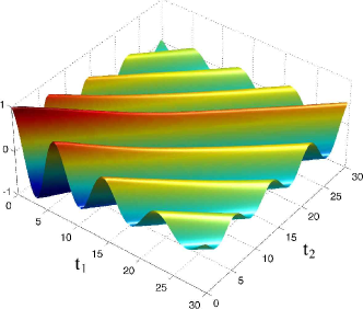
Figure 4: The imaginary part of the lesser Green’s function $\mbox{\boldmath$\mathcal{G}$}^{<}_{{\rm CC},HH}(t_{1},t_{2})$ of the central region in molecular orbital basis corresponding to the HOMO level of the central chain. Bias voltage $U=1.2$, HF approximation.

In Fig. 4 we display the imaginary part of $\mbox{\boldmath$\mathcal{G}$}^{<}_{{\rm CC},HH}(t,t^{\prime})$ in the basis of the initial Hartree-Fock molecular orbitals, for an applied bias $U=1.2$. This matrix element corresponds to the HOMO level of the molecular chain. The value of the Green’s function on the time diagonal, i.e., $n_{H}(t)={\rm Im}[\mbox{\boldmath$\mathcal{G}$}^{<}_{{\rm CC},HH}(t,t)]$ gives the level occupation number per spin. We see that $n_{H}(t)$ decays from a value of $1.0$ at the initial time to a value of $0.5$ at time $t=30$. An analysis of the LUMO level occupation $n_{L}(t)$ shows that almost all the charge is transferred to this level. The discharging of the HOMO level and the charging of the LUMO level is also clearly observable in the dipole moment as it causes a density oscillation in the system (see Section III.3). When we move away from the time-diagonal we consider the time-propagation of holes in the HOMO level. We observe a damped oscillation the frequency of which corresponds to the removal energy of an electron from the HOMO level, leading to a distinct peak in the spectral function (see Section III.2 below).

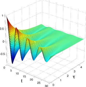
Figure 5: The imaginary part of the mixed Green’s function $\mbox{\boldmath$\mathcal{G}$}^{\rceil}_{{\rm CC},HH}(t,\tau)$ of the central region in molecular orbital basis. Bias voltage $U=1.2$, HF approximation.

The imaginary part of $\mbox{\boldmath$\mathcal{G}$}^{\rceil}_{{\rm CC},HH}(t,\tau)$ within the HF approximation is displayed in Fig. 5 for real times between $t=0$ and $t=30$ and imaginary times from $\tau=0$ to $\tau=5$. This mixed-time Green’s function accounts for initial correlations as well as initial embedding effects (within the HF approximation only the latter). At $t=0$ we have the ground-state Matsubara Green’s function and as the real time $t$ increases all elements of $\mbox{\boldmath$\mathcal{G}$}^{\rceil}_{\rm CC}(t,\tau)$ approach zero independently of the value of $\tau$. This behavior indicates that initial effects die out in the long-time limit and that the decay rate is directly related to the time for reaching a steady state. A very similar behavior is found within the 2B and GW approximation but with a stronger damping of the oscillations.

III.2 Time-dependent current

The time-dependent current at the right interface between the chain and the two-dimensional lead is shown in Fig. 6 for the HF, 2B and GW approximations for two different values of the applied bias $U=0.8$ (weak) and $1.2$ (strong).

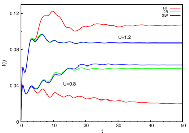
Figure 6: Transient currents flowing into the right lead for the HF, 2B and GW approximations with the applied bias $U=0.8$ (three lowest curves) and $U=1.2$.

The first remarkable feature is that the 2B and GW results are in excellent agreement at all times both in the weak and strong bias regime while the HF current deviates from the correlated results already after few time units. This result indicates that a chain of 4 atoms is already long enough for screening effects to play a crucial role. The 2B and GW approximations have in common the first three diagrams of the perturbative expansion of the many-body self-energy illustrated in Fig. 3. We thus conclude that the first order exchange diagram (Fock) with an interaction screened by an electron-hole propagator with a single polarization bubble (with fully dressed Green’s functions) contains the essential physics of the problem. We also wish to emphasize that the 2B approximation includes the so called second-order exchange diagram which is also quadratic in the interaction. This diagram is less relevant due to the restricted phase-space that two electrons in the chain have to scatter and exchange.

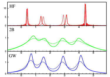
Figure 7: Spectral functions $A(\omega)$ for HF (uppermost plot), 2B (middle plot) and GW (bottom plot) approximation with the applied bias $U=0.8$ (solid line) and $U=1.2$ (dashed line).

We then turn our attention to the spectral function which is defined as

$$A(T,\omega)=-{\rm Im}{\rm Tr}_{\rm C}\int\frac{dt}{2\pi}\,e^{i\omega t}[\mbox{\boldmath$\mathcal{G}$}_{\rm CC}^{>}-\mbox{\boldmath$\mathcal{G}$}_{\rm CC}^{<}](T+\frac{t}{2},T-\frac{t}{2}).$$ (40)

For values of $T$ after the transients have died out the spectral function becomes independent of $T$. For such times we denote the spectral function by $A(\omega)$ and it is easy to show that $A(\omega)={\rm Tr}_{\rm C}[{\bf A}(\omega)]$ where ${\bf A}(\omega)$ is defined in Eq. (35). This function displays peaks that correspond to removal energies (below the chemical potential) and electron addition energies (above the chemical potential). The spectral functions of our system are displayed in Fig. 7. At weak bias the HOMO-LUMO gap in the HF approximation is fairly the same as the equilibrium gap whereas the 2B and GW gaps collapse causing both the HOMO and the LUMO to move in the bias window. As a consequence the steady-state HF current is notably smaller than the 2B and GW currents. This effect has been previously observed by Thygesent.2008 and is confirmed by our time-dependent simulations.

A new scenario does, however, emerge in the strong bias regime. The HF HOMO and LUMO levels move into the bias window and lift the steady-state current above the corresponding 2B and GW values. This can be explained by observing that the peaks of the HF spectral function $A(\omega)$ are very sharp compared to the rather broadened structures in the 2B and GW approximations, see Fig. 7. In the correlated case the HOMO and LUMO levels can be exploited only partially by the electrons to scatter from left to right and we thus observe a suppression of the current with respect to the HF case. From a mathematical point of view the steady-state current is roughly proportional to the integral of $A(\omega)$ over the bias window which is larger in the HF approximation.

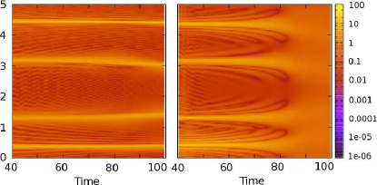
Figure 8: Real-time evolution of the spectral function $A(T,\omega)$ for the HF (left panel) and the 2B approximation (right panel) for an applied bias of $U=1.2$. On the horizontal axis the time $T$ and the vertical axis the frequency $\omega$.

The time-evolution of the spectral function $A(T,\omega)$ as a function of $T$ is illustrated in Fig. 8 for the case of the HF and the 2B approximation. For these results, the ground state system was propagated without bias up to $T=40$ after which a bias was suddenly turned on. The HF peaks remain rather sharp during the entire evolution and the HOMO-LUMO levels come nearer to each other at a constant speed. On the contrary, the broadening of the 2B peaks remains small during the initial transient regime (up to $T=70$) to then increase dramatically. This behavior indicates that there is a critical charging time after which an enhanced renormalization of quasiparticle states takes place causing a substantial reshaping of the equilibrium spectral function.

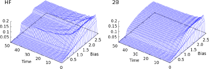
Figure 9: Transient right current $I_{\rm R}(U,t)$ as a function of applied bias voltage and time in the HF (left panel) and 2B (right panel) approximations.

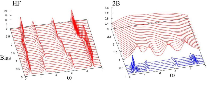
Figure 10: Spectral function $A(\omega)$ for the HF (left panel) and 2B (right panel) approximation, as a function of the bias voltage. For the 2B approximation the spectral functions for bias voltages until $U=0.6$ were divided by a factor 30 (blue lines in the figure)

The time-dependent current at the right interface as a function of applied voltage and time is shown in Fig. 9 for the HF and 2B approximation. The figures nicely illustrate how steady state results are obtained from time-dependent calculations: after the transients have died out we see the formation of the characteristic I-V curves familiar from steady state transport calculations. In the HF approximation one clearly observes the typical staircase structure with steps that correspond to an applied voltage that includes one more resonance in the bias window. These steps appear at bias voltages $U=0.9$ and $U=1.8$. This result is corroborated by the left panel of Fig. 10 in which we display the bias-dependent spectral function for the HF approximation. Here we see a sudden shift in the spectral peaks at these voltages. The HF results thus bear a close resemblance to the standard non-interacting results, the main difference being that the HF position of the levels gets renormalized by the applied bias.

We now turn our attention to the 2B approximation in the right panel of Fig.9. We notice a clear step at bias voltage of $U=0.7$ but the broadening of the level peaks due to quasiparticle collisions completely smears out the second step and the current increases smoothly as a function of the applied voltage. This is again corroborated in the right panel of Fig.10 where we observe a sudden broadening of the spectral function at a bias of $U=0.7$. To make this effect clearly visible in the figure we divided the spectral functions for biases up to $U=0.6$ by a factor of $30$. We further notice that for the 2B approximation there is a faster gap closing as a function of the bias voltage as compared to the HF approximation. Very similar results are obtained within the GW approximation. We can therefore conclude that electronic correlations beyond Hartree-Fock level have a major impact on both transient and steady-state currents.

III.3 Time-dependent dipole moment

To study how the charge redistribute along the chain after a bias voltage is switched on we calculated the time-dependent dipole moment

$$d(t)=\sum_{i=1}^{4}x_{i}n_{i}(t)$$ (41)

where the $x_{i}$ are the coordinates of the sites of the chain (with a lattice spacing of one) with origin between sites 2 and 3. As observed in Section III.1 the chain remains fairly charge neutral during the entire time evolution. However, a charge rearrangement occurs as can be seen from Fig. 11. At $U=1.2$ both the HOMO and the LUMO are inside the bias window, the lowest level remains below and the highest level above. Electrons in the initially populated HOMO then move to the empty LUMO and get only partially reflected back. This generates damped oscillations with the HOMO-LUMO gap as the main frequency, a non-vanishing steady value for the LUMO population and a partially filled HOMO. Due to the different (odd/even) approximate spatial symmetry of the HOMO/LUMO levels a net dipole moment develops.

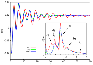
Figure 11: Dipole moment of the central region as a function of time for bias $U=1.2$. The inset shows the Fourier transform of the dipole moment.

As we pointed out in a recent Letter,mssvl.2008 the oscillations in the transient current reflect the electronic transitions between the ground state levels of the central region and the electrochemical potentials of the left and right leads. However, the oscillations are visible in all observable quantities through the oscillations of the Green’s function discussed in Section III.1. Detailed information on the electronic level structure of the chain can be extracted from the Fourier transform of $d(t)$, see inset in Fig. 11. One clearly recognize the presence of sharp peaks superimposed to a broad continuum. The peaks occur at energies corresponding to electronic transitions from lead states at the left/right electrochemical potential to chain eigenstates or to intrachain transitions. We will denote a transition energy between leads ${\rm L}$ and ${\rm R}$ and chain eigenstate $i$ by $\Delta\epsilon_{{\rm L}i}$ and $\Delta\epsilon_{i{\rm R}}$. Similarly we will denote a transition energy between states in the central region as $\Delta\epsilon_{ij}$. In the inset of Fig. 11 the main peak structures are labeled from the highest to the lowest transition energies with letters (a) to (e) and we will use these labels to denote the various transitions discussed below. The possible transition energies can be determined form the position of the peaks in the spectral functions and the lead levels. As expected the dominant peak occurs at the intrachain transition energy $\Delta\epsilon_{23}\approx 1.5$ (c). This roughly corresponds to the average of the equilibrium and nonequilibrium gaps and, therefore, must be traced back to charge fluctuations between the HOMO and LUMO. The other observable transition energies are $\Delta\epsilon_{{\rm L}2}\approx 2.0$ (b), $\Delta\epsilon_{{\rm L}3}\approx 0.5$ (e) and $\Delta\epsilon_{{\rm L}4}\approx 1.0$ (d) from the left lead and $\Delta\epsilon_{1{\rm R}}\approx 0.65$ (e), $\Delta\epsilon_{2{\rm R}}\approx 0.4$ (e), $\Delta\epsilon_{3{\rm R}}\approx 2.0$ (b) and $\Delta\epsilon_{4{\rm R}}\approx 3.4$ (a) from the right lead. Some of the peaks with transition energies close to each other ($\Delta\epsilon_{{\rm L}2}$ & $\Delta\epsilon_{3{\rm R}}$ (b) and $\Delta\epsilon_{{\rm L}3}$ & $\Delta\epsilon_{1{\rm R}}$ & $\Delta\epsilon_{2{\rm R}}$(e)) are merged together and broadened. The broadening is not only due to embedding and many-body effects but also to the dynamical renormalization of the position of the energy levels. Further information can be extracted from the peak intensities. The peak of the $\Delta\epsilon_{{\rm L}4}$ (d) transition is very strong due to the sharpness of that particular resonance, see Fig. 7, and its initial low population. On the contrary, the transition $\Delta\epsilon_{{\rm L}1}$ from the left lead to the highly populated level $\epsilon_{1}$ is extremely weak due to the Pauli blockade and not visible. Correlation effects beyond Hartree-Fock theory causes a fast damping of all sofar discussed transitions. Only the transitions $\Delta\epsilon_{{\rm L}4}$ (d) and $\Delta\epsilon_{23}$ (c) are visible in the Fourier spectrum of the 2B and GW approximation.

III.4 Time dependent screened interaction $W$

In Fig. 12 we show the trace of the lesser component of the time-dependent screened interaction of the GW approximation in the double-time plane. This interaction is defined as $W=v+v\,P\,W$ where $P$ is the full polarization bubblesdvl.2009 (with dressed Green’s functions) of the connected and correlated system, and gives information on the strength and efficiency of the dynamical screening of the repulsive interactions. The good agreement between the 2B and GW approximations implies that the dominant contribution to the screening comes from the first bubble diagram, that is $W^{<}\approx vP^{<}v$. From Fig. 12 we see that the trace of the imaginary part of $W^{<}(t,t)$ is about 3. Considering that the trace of the instantaneous bare interaction $v$ is 6 we conclude that the screening diagrams reduce the magnitude of the repulsion by a factor of 2. Another interesting feature of the screened interaction is that it decays rather fast when the separation of the time arguments increases. From Fig. 12 we see that after a time $t\approx 7$ the retarded interaction is negligibly small. It is worth noting that such a time scale is much smaller than the typical time scales to reach a steady state, see Fig. 6.

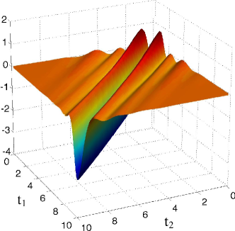
Figure 12: Imaginary part of the trace of the screened interaction $W^{<}(t_{1},t_{2})$ in the GW approximation.

III.5 Time-dependent Friedel oscillations in the leads

We implemented the method described in Section II.5 and based on the inbedding technique to investigate the electron dynamics in the leads. This study is of special importance since it challenges one of the main assumption in quantum transport calculations, i.e., that the leads remain in thermal equilibrium during the entire evolution.

In Fig. 13 we show the evolution of the density in the two-dimensional 9-row wide leads (see Fig. 1) after the sudden switch-on of a bias voltage. We display snapshots of the lead densities at times $t=0,1.7,3.6$ and $10$ where up to 10 layers deep into the leads (where to improve the visibility we interpolated the density between the sites). Since the atomic wire is connected to the central site it acts as an impurity and we see density oscillations in the leads following diamond-like pattern. These present Friedel oscillations that propagate along preferred directions.

The preferred directions in the density pattern can be understood from linear response theory. Given a square lattice with nearest neighbor hopping $T=T^{\lambda}=T^{\tau}$ the retarded density response function in Fourier space reads

$$\chi({\bf q},\omega) = \int\frac{d{\bf k}}{(2\pi)^{2}}\frac{f(\epsilon_{{\bf k}})-f(\epsilon_{{\bf k}+{\bf q}})}{\omega-\epsilon_{{\bf k}}+\epsilon_{{\bf k}+{\bf q}}+i\eta}$$ (42)

$$= 2\int\frac{d{\bf k}}{(2\pi)^{2}}\frac{f(\epsilon_{{\bf k}})(\epsilon_{{\bf k}}-\epsilon_{{\bf k}+{\bf q}})}{(\omega+i\eta)^{2}-(\epsilon_{{\bf k}}-\epsilon_{{\bf k}+{\bf q}})^{2}},$$

where $\epsilon_{{\bf k}}=2T(\cos k_{x}+\cos k_{y})$ is the energy dispersion and the integral is done over the first Brillouin zone and $f$ is the Fermi distribution function. At half filling the Fermi energy is zero and the Fermi surface is a square with vertices in $(0,\pm\pi)$ and $(\pm\pi,0)$. The dominant contribution to the integral comes from the values of ${\bf k}$ close to such vertices where the density of states has van Hove singularities. The response function $\chi({\bf q}=\alpha{\bf Q},\omega=0)$, with ${\bf Q}=(\pi,\pi)$ the nesting vector, is discontinuous for $\alpha=1$. Indeed, for every occupied ${\bf k}$ there exists an $\alpha<1$ such that $\epsilon_{{\bf k}+{\bf q}}=\epsilon_{{\bf k}}<0$ and the integrand diverges at zero frequency. On the other hand for $\alpha>1$ the vector ${\bf k}+{\bf q}$ corresponds to an unoccupied state with energy $\epsilon_{{\bf k}+{\bf q}}>0$ and due to the presence of the Fermi function the integrand of Eq.(42) is well behaved even for $\omega=0$. The discontinuity at ${\bf Q}=(\pi,\pi)$ is analogous to the discontinuity at $2k_{F}$ in the electron gas and leads to the Friedel oscillations with diamond symmetry observed in Fig. 13. By adding reciprocal lattice vectors we find that there are four equivalent directions for these Friedel oscillations given by the vectors ${\bf Q}=\pm(\pi,\pm\pi)$. Each of these vectors gives in real space rise to a density change of the form $\delta n(\mathbf{r})\sim e^{{i\mathbf{Q}}\cdot\mathbf{r}}$. Therefore a single impurity in a 2D lattice induces a cross-shaped density pattern. Due to the fact that in our case the lattice ends at the central chain, we only observe two arms of this cross.

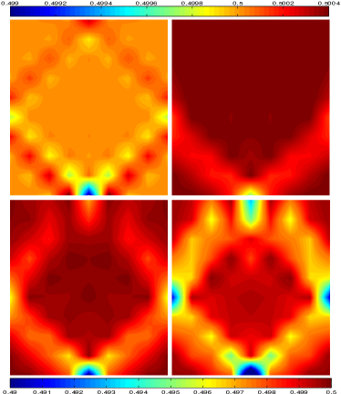
Figure 13: Snapshots of the density in left lead for HF approximation after the bias $U=1.2$ switch-on. On the horizontal axes the transverse dimension of the lead (9 rows wide, with the site connected to the chain in the center) and 10 layers deep. Upper panel left: Initial density, Upper panel right: density at time $t=1.7$, Lower left panel: density at time $t=3.6$, Lower right panel: density at time $t=10$. The upper colorbar refers to the initial density in the upper left panel. The lower colorbar refers to the remaining pictures.

The results of Fig. 13 also allows for testing the assumption of thermal equilibrium in the leads. The equilibrium density [Top-left panel] is essentially the same as its equilibrium bulk value at 0.5. After the switching of the bias a density corrugation with the shape of a diamond starts to propagate deep into the lead. The largest deviation from the bulk density value occurs at the corners of the diamond and is about $2\%$ at the junction while it reduces to about $1\%$ after 10 layers. We also verified that the discrepancy is about 3 times larger for leads with only three transverse channels. We conclude that the change in the lead density goes like the inverse of the cross section. Our results suggests that for a mean field description of 2D leads with 9 transverse channels it is enough to include few atomic layers for an accurate self-consistent time-dependent calculations of the Hartree potential.

IV Conclusions

We proposed a time-dependent many-body approach based on the real-time propagation of the KB equations to tackle quantum transport problems of correlated electrons. We proved the continuity equation for any $\Phi$-derivable self-energy, a fundamental property in non-equilibrium conditions, and generalize the Meir-Wingreen formula to account for initial correlations and initial embedding effects. This requires an extension of the Keldysh contour with the thermal segment $(t_{0},t_{0}-i\beta)$ and the consideration of mixed-time Green’s functions having one real and one imaginary time argument. The Keldysh Green’s function in the device region $\mbox{\boldmath$\mathcal{G}$}_{\rm{CC}}$ is typically used to calculate currents and densities in the device. In this work we also developed an exact inbedding scheme to extract from $\mbox{\boldmath$\mathcal{G}$}_{\rm{CC}}$ the TD density in the leads.

The theoretical framework and the implementation scheme were tested for one-dimensional wires connected to two-dimensional leads using different approximations for the many-body self-energy. We found that already for 4-sites wires screening effects play a crucial role. The 2B and GW approximations are in excellent agreement at all times for moderate interaction strength (of the same order of magnitude of the hopping integrals) while the HF approximation tends to deviate from the GW and 2B results after very short times. These differences were related to the sharp peaks of the HF spectral function as compared to the rather broad structures observed in 2B and GW. Our numerical results indicate that the largest part of the correlation effects are well described by the first bubble diagram of the self-energy, common to both the 2B and GW approximation. The screened interaction was explicitely calculated in the GW approximation showing that the screening reduces the interaction strenght by a factor of 2 and that retardation effects are absent after a time-scale much shorter than the typical transient time-scale. The electron dynamics obtained using a correlated self-energy differ from the HF dynamics in many respects: 1) At moderate bias the HOMO-LUMO gap closes while in the HF approximation it remains fairly constant; 2) The HOMO and LUMO resonances are rather sharp during the transient time to then suddenly broaden when approaching the steady state. This indicates the occurrence of an enhanced renormalization of quasiparticle states. The HF widths instead remain unaltered. 3) The transient time in the correlated case is much shorter than in HF, see Fig. 11.

The transient behavior of time-dependent quantities like the current and dipole moment exhibit oscillations of characteristic frequencies that reflect the underlying level-structure of the system. Calculating the ultrafast response of the device to an external driving field thus constitutes an alternative method to gain insight into the quasi-particle positions and life-times out of equilibrium. We performed a discrete Fourier analysis of the TD dipole-moment in the transient regime and related the characteristic frequencies to transitions either between different levels of the wire or between the levels of the wire and the electrochemical potential of the leads. The hight of the peaks in the Fourier transform can be interpreted as the amount of density which oscillate between the levels of a given transition. In all approximations we found that the density mainly sloshes between the HOMO and the LUMO.

One of the main assumption in quantum transport calculations is that the leads remain in thermal equilibrium and therefore that the bulk density is not affected by the presence of the junction. To investigate this assumption we considered two-dimensional leads thus going beyond the so called wide-band-limit approximation. By virtue of an exact inbedding technique we calculated the lead density both in and out equilibrium. In the proximity of the junction the density exhibits Friedel-like oscillations whose period depend on the value of the Fermi momentum along the given direction.

In conclusion the real-time-propagation of the KB equations for open and inhomogeneous systems provide a very powerful tool to study the electron dynamics of a typical quantum transport set-up. In this work we considered only DC biases. However, more complicated driving fields like AC biases or pumping fields can be dealt with at the same computational cost and the results will be the subject of a future publication. Besides currents and densities the MBPT framework also allows for calculating higher order correlators. It is our intention to use the KB equations to study shot-noise in quantum junctions using different levels of approximation for the Green’s function.

Appendix A The embedded Kadanoff-Baym equations

To apply Eq. (22) in practice we need to transform it to real-time equations that we solve by time-propagation. This can be done in Eq. (22) by considering time-arguments of the Green’s function and self-energy on different branches of the contour. We therefore have to define these components first. Let us therefore consider a function on the Keldysh contour of the general form

$$F(z,z^{\prime}) = F^{\delta}(z)\delta(z,z^{\prime})$$ (43)

$$+ \theta(z,z^{\prime})F^{>}(z,z^{\prime})+\theta(z^{\prime},z)F^{<}(z,z^{\prime}),$$

where $\theta(z,z^{\prime})$ is a contour Heaviside function,d.1984 i.e. $\theta(z,z^{\prime})=1$ for $z$ later than $z^{\prime}$ on the contour and zero otherwise, and $\delta(z,z^{\prime})=\partial_{z}\theta(z,z^{\prime})$ is the contour delta function. By restricting the variables $z$ and $z^{\prime}$ on different branches of the contour we can define the various components of $F$ as

$$F^{\lessgtr}(t,t^{\prime}) = F(t_{\mp},t_{\pm}^{\prime}),$$ (44)

$$F^{\rceil}(t,\tau) = F(t_{\pm},t_{0}-i\tau),$$ (45)

$$F^{\lceil}(\tau,t) = F(t_{0}-i\tau,t_{\pm}),$$ (46)

$$F^{M}(\tau-\tau^{\prime}) = -iF(t_{0}-i\tau,t_{0}-i\tau^{\prime}),$$ (47)

and

$$F^{R/A}(t,t^{\prime})=F^{\delta}(t)\delta(t-t^{\prime})\mp\theta(\pm t\mp t^{\prime})[F^{>}(t,t^{\prime})-F^{<}(t,t^{\prime})].$$ (48)

For the Green’s function there is no singular contribution, i.e., $\mbox{\boldmath$\mathcal{G}$}^{\delta}=0$, but the self-energy has a singular contribution of Hartree-Fock form, i.e., $\mbox{\boldmath$\Sigma$}^{\delta}=\mbox{\boldmath$\Sigma$}^{\rm HF}[\mbox{\boldmath$\mathcal{G}$}]$.d.1984 With these definitions we can now convert Eq. (22) to equations for the separate components. This is conveniently done using the conversion table in Ref. TDDFTbook, . We then obtain the following set of equations

$$i\partial_{t}\mbox{\boldmath$\mathcal{G}$}^{\lessgtr}(t,t^{\prime}) = \mathbf{H}_{\rm{CC}}(t)\mbox{\boldmath$\mathcal{G}$}^{\lessgtr}(t,t^{\prime})+\left[\mbox{\boldmath$\Sigma$}^{R}\cdot\mbox{\boldmath$\mathcal{G}$}^{\lessgtr}\right](t,t^{\prime})$$

$$+ \left[\mbox{\boldmath$\Sigma$}^{\lessgtr}\cdot\mbox{\boldmath$\mathcal{G}$}^{A}\right](t,t^{\prime})+\left[\mbox{\boldmath$\Sigma$}^{\rceil}\star\mbox{\boldmath$\mathcal{G}$}^{\lceil}\right](t,t^{\prime}),$$

$$-i\partial_{t^{\prime}}\mbox{\boldmath$\mathcal{G}$}^{\lessgtr}(t,t^{\prime}) = \mbox{\boldmath$\mathcal{G}$}^{\lessgtr}(t,t^{\prime})\mathbf{H}_{\rm{CC}}(t^{\prime})+\left[\mbox{\boldmath$\mathcal{G}$}^{R}\cdot\mbox{\boldmath$\Sigma$}^{\lessgtr}\right](t,t^{\prime})$$

$$+ \left[\mbox{\boldmath$\mathcal{G}$}^{\lessgtr}\cdot\mbox{\boldmath$\Sigma$}^{A}\right](t,t^{\prime})+\left[\mbox{\boldmath$\mathcal{G}$}^{\rceil}\star\mbox{\boldmath$\Sigma$}^{\lceil}\right](t,t^{\prime}),$$

$$i\partial_{t}\mbox{\boldmath$\mathcal{G}$}^{\rceil}(t,\tau) = \mathbf{H}_{\rm CC}(t)\mbox{\boldmath$\mathcal{G}$}^{\rceil}(t,\tau)+\left[\mbox{\boldmath$\Sigma$}^{R}\cdot\mbox{\boldmath$\mathcal{G}$}^{\rceil}\right](t,\tau)$$ (51)

$$+ \left[\mbox{\boldmath$\Sigma$}^{\rceil}\star\mbox{\boldmath$\mathcal{G}$}^{\mathrm{M}}\right](t,\tau),$$

$$-i\partial_{t}\mbox{\boldmath$\mathcal{G}$}^{\lceil}(\tau,t) = \mbox{\boldmath$\mathcal{G}$}^{\lceil}(\tau,t)\mathbf{H}_{\rm CC}(t)+\left[\mbox{\boldmath$\mathcal{G}$}^{\lceil}\cdot\mbox{\boldmath$\Sigma$}^{A}\right](\tau,t)$$ (52)

$$+ \left[\mbox{\boldmath$\mathcal{G}$}^{M}\star\mbox{\boldmath$\Sigma$}^{\lceil}\right](\tau,t),$$

$$-\partial_{\tau}\mbox{\boldmath$\mathcal{G}$}^{M}(\tau-\tau^{\prime}) = \mathbf{1}\delta(\tau-\tau^{\prime})+\mathbf{H}_{\rm{CC}}\mbox{\boldmath$\mathcal{G}$}^{M}(\tau-\tau^{\prime})$$ (53)

$$+ i\left[\mbox{\boldmath$\Sigma$}^{M}\star\mbox{\boldmath$\mathcal{G}$}^{\mathrm{M}}\right](\tau-\tau^{\prime}),$$

which are commonly known as the Kadanoff-Baym equations. The symbols $\cdot$ and $\star$ are a shorthand notation for the real-time and imaginary-time convolutions

$$\begin{split}&\left[a\cdot b\right](t,t^{\prime})=\int_{0}^{\infty}a(t,\bar{t})b(\bar{t},t^{\prime})d\bar{t},\\ &\left[a\star b\right](t,t^{\prime})=-i\int_{0}^{\beta}a(t,\tau)b(\tau,t^{\prime})d\tau.\end{split}$$ (54)

In practice we first solve Eq. (53) which describes the initial equilibrium Green’s function. This equation is decoupled from the other two, since $\mbox{\boldmath$\Sigma$}^{M}$ depends on $\mbox{\boldmath$\mathcal{G}$}^{M}$ only. The initial conditions for the other Green’s functions $G^{\lessgtr}$ and $G^{\rceil\lceil}$ are then determined by $\mbox{\boldmath$\mathcal{G}$}^{M}$ as follows

$$\mbox{\boldmath$\mathcal{G}$}^{>}(0,0) = i\mbox{\boldmath$\mathcal{G}$}^{M}(0^{+}),$$ (55)

$$\mbox{\boldmath$\mathcal{G}$}^{<}(0,0) = i\mbox{\boldmath$\mathcal{G}$}^{M}(0^{-}),$$ (56)

$$\mbox{\boldmath$\mathcal{G}$}^{\rceil}(0,\tau) = i\mbox{\boldmath$\mathcal{G}$}^{M}(-\tau),$$ (57)

$$\mbox{\boldmath$\mathcal{G}$}^{\lceil}(\tau,0) = i\mbox{\boldmath$\mathcal{G}$}^{M}(\tau).$$ (58)

With these initial conditions the Eqs.(LABEL:eq:kb1)-(52) can be solved using a time-stepping algorithm.sdvl.2009b

Appendix B Embedding self-energy

From Eq. (21) and Eq. (13) we see that the embedding self-energy has the form

$$\mbox{\boldmath$\Sigma$}_{{\rm em},\alpha,kl}(z,z^{\prime})=\sum_{ij}V_{k,i\alpha}\mbox{\boldmath$g$}_{\alpha\alpha,ij}(z,z^{\prime})V_{j\alpha,l},$$ (59)

where $k$ and $l$ label orbitals in the central region. As can be seen from this equation, the calculation of the embedding self-energy requires the determination of $\mbox{\boldmath$g$}_{\alpha\alpha}$. Since for the isolated lead $\alpha$ the time-dependent field is simply a gauge, $\mbox{\boldmath$g$}_{\alpha\alpha}$ is of the form

$$\mbox{\boldmath$g$}_{\alpha\alpha}(z,z^{\prime})=\mbox{\boldmath$g$}_{\alpha\alpha}^{0}(z,z^{\prime})\exp\left(-i\int_{z^{\prime}}^{z}d\bar{z}\,U_{\alpha}(\bar{z})\right),$$ (60)

where $\mbox{\boldmath$g$}_{\alpha\alpha}^{0}$ is the Green’s function for the unbiased lead, and the integral in the exponent is a contour integral. The Green’s function $\mbox{\boldmath$g$}^{0}_{\alpha\alpha}$ has the form

$$\mbox{\boldmath$g$}_{\alpha\alpha}^{0}(z,z^{\prime})=\theta(z,z^{\prime})\mbox{\boldmath$g$}^{0,>}_{\alpha\alpha}(z,z^{\prime})+\theta(z^{\prime},z)\mbox{\boldmath$g$}^{0,<}_{\alpha\alpha}(z,z^{\prime}).$$ (61)

It therefore remains to specify $\mbox{\boldmath$g$}^{0,\lessgtr}_{\alpha\alpha}$. In the following we will for convenience separate out the spin part from the Green’s function and write $\mbox{\boldmath$g$}^{0}_{\alpha\alpha,i\sigma,j\sigma^{\prime}}=\delta_{\sigma\sigma^{\prime}}\mbox{\boldmath$g$}^{0}_{\alpha\alpha,ij}$. We will now give give an explicit expression for $\mbox{\boldmath$g$}^{0}_{\alpha\alpha,ij}$ for the case of two-dimensional leads. The case of three dimensions can be treated similarly. We consider a lead Hamiltonian of a tight-binding form, that is separable in the longitudinal ($x$) and the transverse ($y$) directions. Therefore the indices in the one-particle matrix $h_{ij}^{\alpha}$ of Eq. (3) denote sites $i=(x,y),j=(x^{\prime},y^{\prime})$ where $x$ and $y$ are integers running from zero to $N_{x}^{\alpha}$ and $N_{y}^{\alpha}$. At the end of the derivation we take the limit $N_{x}^{\alpha}\rightarrow\infty$. The Hamiltonian matrix for the leads is then of the form

$$h^{\alpha}_{ij}(t)=\delta_{xx^{\prime}}\tau^{\alpha}_{yy^{\prime}}+\delta_{yy^{\prime}}\lambda^{\alpha}_{xx^{\prime}}+a^{\alpha}\delta_{ij},$$ (62)

where $\lambda$ and $\tau$ are matrices that represent longitudinal and transverse chains and $a^{\alpha}$ is an on-site energy. Hence

$$\mbox{\boldmath$g$}_{\alpha\alpha,ij}^{0,\lessgtr}(z,z^{\prime})=\sum_{p}U^{\alpha}_{ip}\,\mbox{\boldmath$g$}^{0,\lessgtr}_{\alpha\alpha,p}(z,z^{\prime})U_{pj}^{\alpha\dagger},$$ (63)

where $p=(p_{x},p_{y})$ is a two-dimensional index spanning the same one-particle space. The matrix $U^{\alpha}=D^{\tau\alpha}\otimes D^{\lambda\alpha}$ is a direct product of the unitary matrices $D^{\tau\alpha}$ and $D^{\lambda\alpha}$ that diagonalize the matrices $\tau^{\alpha}$ and $\lambda^{\alpha}$ in Eq. (62) The functions $\mbox{\boldmath$g$}^{0,\lessgtr}_{\alpha\alpha,p}$ have the explicit form

$$\mbox{\boldmath$g$}_{\alpha\alpha,p}^{0,<}(z,z^{\prime}) = if(\epsilon_{p\alpha})e^{-i\int_{z^{\prime}}^{z}d\bar{z}\,(\epsilon_{p\alpha}-\mu)},$$ (64)

$$\mbox{\boldmath$g$}_{\alpha\alpha,p}^{0,>}(z,z^{\prime}) = i(f(\epsilon_{p\alpha})-1)e^{-i\int_{z^{\prime}}^{z}d\bar{z}\,(\epsilon_{p\alpha}-\mu)},$$ (65)

with $f(\epsilon)=1/(e^{\beta(\epsilon-\mu)}+1)$ the Fermi distribution function. In these expressions $\epsilon_{p\alpha}=\epsilon_{p_{y}\alpha}^{\tau}+\epsilon_{p_{x}\alpha}^{\lambda}$, where $\epsilon_{p_{y}\alpha}^{\tau}$ and $\epsilon_{p_{x}\alpha}^{\lambda}$ are the eigenvalues of matrices $\tau^{\alpha}$ and $\lambda^{\alpha}$.

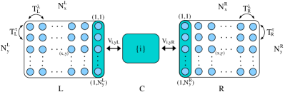
Figure 14: Tight-binding system for finite 2D leads connected to scattering central region.

In the case the matrices $\tau^{\alpha}$ and $\lambda^{\alpha}$ represent tight-binding chains with nearest neigbour hoppings $T_{\alpha}^{\tau}$ and $T_{\alpha}^{\lambda}$ and zero on-site energy, we have

$$D^{\lambda\alpha}_{xp_{x}} = \sqrt{\frac{2}{N_{x}^{\alpha}+1}}\sin(\frac{\pi xp_{x}}{N_{x}^{\alpha}+1}),$$ (66)

$$\epsilon_{p_{x}\alpha}^{\lambda} = 2T_{\alpha}^{\lambda}\cos(\frac{\pi p_{x}}{N_{x}^{\alpha}+1}),$$ (67)

and similarly for the transverse transformation matrix $D^{\tau\alpha}_{yp_{y}}$ and energy $\epsilon_{p_{y}\alpha}^{\tau}$. If we insert these expressions in Eq. (63) and take the limit $N_{x}\rightarrow\infty$ such that we can replace summation over $p_{x}$ by an integration over the angular variable $\phi=\pi p_{x}/(N_{x}^{\alpha}+1)$, then we obtain

$$\mbox{\boldmath$g$}_{\alpha\alpha,ij}^{0,<}(z,z^{\prime}) = \frac{4i}{N_{y}^{\alpha}+1}\sum_{p_{y}=1}^{N_{y}^{\alpha}}\sin(\frac{\pi yp_{y}}{N_{y}^{\alpha}+1})\sin(\frac{\pi y^{\prime}p_{y}}{N_{y}^{\alpha}+1})$$ (68)

$$\times \frac{1}{\pi}\int_{0}^{\pi}d\phi\sin(x\phi)\sin(x^{\prime}\phi)$$

$$\times f(\epsilon_{p\alpha})e^{-i\int_{z^{\prime}}^{z}d\bar{z}\,(\epsilon_{p\alpha}-\mu)},$$

where now

$$\epsilon_{p\alpha}=a^{\alpha}+2T_{\alpha}^{\tau}\cos(\frac{\pi p_{y}}{N_{y}^{\alpha}+1})+2T_{\alpha}^{\lambda}\cos\phi.$$ (69)

The expression for $\mbox{\boldmath$g$}_{\alpha\alpha,ij}^{0,>}$ is obtained from Eq. (68) by simply replacing the Fermi function $f$ by $f-1$. Let us now turn to the embedding self-energy. In this work we consider the case that we only have hopping elements $V_{i,k\alpha}$ between central sites $i$ and the first tranverse layer of the leads, which are labeled by elements $k=(1,y)$ where $y=1\ldots N_{y}^{\alpha}$. However, the entire formalism can extended to more general cases. This means that we take

$$V_{i,k\alpha}=\left\{\begin{array}[]{cc}V_{i,y\alpha}&\mbox{if $k=(1,y)$}\\ 0&\mbox{otherwise}\end{array}\right..$$ (72)

In that case in Eq. (68) only the contribution with $x=x^{\prime}=1$ survives. Then the product of the sine functions can be written in terms of the eigenenergies of the isolated leads as

$$\mbox{\boldmath$\Sigma$}_{{\rm em},\alpha,kl}^{<}(z,z^{\prime}) = \sum_{y,y^{\prime},p_{y}=1}^{N_{y}^{\alpha}}\frac{4iV_{k,y\alpha}V_{y^{\prime}\alpha,l}}{N_{y}^{\alpha}+1}$$ (73)

$$\times \sin(\frac{\pi yp_{y}}{N_{y}^{\alpha}+1})\sin(\frac{\pi y^{\prime}p_{y}}{N_{y}^{\alpha}+1})$$

$$\times \frac{1}{\pi}\int_{E_{p_{y}\alpha}^{-}}^{E_{p_{y}\alpha}^{+}}\frac{d\epsilon}{2|T_{\alpha}^{\lambda}|}\sqrt{1-\left(\frac{E_{p_{y}\alpha}}{2T_{\alpha}^{\lambda}}\right)^{2}}$$

$$\times f(\epsilon)e^{-i\int_{z^{\prime}}^{z}d\bar{z}\,(\epsilon-\mu)},$$

where we defined $E_{p_{y}\alpha}=\epsilon-a^{\alpha}-\epsilon_{p_{y}\alpha}^{\tau}$ and $E_{p_{y}\alpha}^{\pm}=a^{\alpha}+\epsilon_{p_{y}\alpha}^{\tau}\pm 2|T_{\alpha}^{\lambda}|$. The expression for $\mbox{\boldmath$\Sigma$}_{{\rm em},\alpha}^{>}$ is obtained from Eq. (73) by simply replacing the Fermi function $f$ by $f-1$. In the case that there is no transverse coupling, i.e., $T_{\alpha}^{\tau}=0$, the integral is independent of $p_{y}$ and the sum over $p_{y}$ can be performed to yield $\delta_{yy^{\prime}}$. Then the 2D self-energy becomes a sum of self-energies over separate 1D leads.

References

- (1) For a recent overview see, e.g., Introducing Molecular Electronics, edited by G. Cuniberti, G. Fagas, and K. Richter, Lecture Notes in Physics (Springer, New York, 2005).
- (2) E. Runge and E. K. U. Gross, Phys. Rev. Lett. 52, 997 (1984).
- (3) R. van Leeuwen, Phys. Rev. Lett. 82, 3863 (1999).
- (4) G. Stefanucci and C.-O. Almbladh, Phys. Rev.B 69, 195318 (2004).
- (5) G. Stefanucci and C.-O. Almbladh, Europhys. Lett. 67, 14 (2004).
- (6) M. Di Ventra and T. N. Todorov, J. Phys.: Condens. Matter 16, 8025 (2004).
- (7) F. Evers, F. Weigend and M. Koentopp, Phys. Rev. B 69, 235411 (2004).
- (8) G. Vignale and W. Kohn, Phys. Rev. Lett. 77, 2037 (1996).
- (9) G. Vignale, Phys. Rev. B 70, 201102(R) (2004).
- (10) N. Sai, M. Zwolak, G. Vignale and M. Di Ventra, Phys. Rev. Lett. 94, 186810 (2005).
- (11) M. Koentopp, K. Burke and F. Evers, Phys. Rev. B 73, 121403(R) (2006).
- (12) J. Jung, P. Bokes, and R. W. Godby, Phys. Rev. Lett. 98, 259701 (2007).
- (13) C. Toher, A. Filippetti, S. Sanvito, and K. Burke, Phys. Rev. Lett 95, 146402 (2005).
- (14) J. J. Palacios, Phys. Rev. B 72, 125424 (2005).
- (15) P. Schmitteckert and F. Evers, Phys. Rev. Lett. 100, 086401 (2008).
- (16) R. Stadler, V. Geskin, and J. Cornil, Phys. Rev. B 78, 113402 (2008).
- (17) M. Di Ventra, S. T. Pantelides and N. D. Lang, Phys. Rev. Lett. 84, 979 (2000).
- (18) K. Stokbro, J. Taylor, M. Brandbyge, J.-L. Mozos, and P. Ordejòn, Comput. Mater. Sci. 27, 151 (2003).
- (19) S. Y. Quek, L. Venkataraman, H. J. Choi, S. G. Louie, M. S. Hybertsen, and J. B. Neaton, Nano Lett. 7, 3477 (2007).
- (20) S.-H. Ke, H. U. Baranger and W. Yang, J. Chem. Phys. 126, 201102 (2007)
- (21) Y. Meir and N. S. Wingreen, Phys. Rev. Lett. 68, 2512 (1992).
- (22) A.P.Jauho, N.S.Wingreen and Y.Meir, Phys.Rev.B50, 5528 (1994).
- (23) R. Landauer, IBM J. Res. Dev. 1, 233 (1957).
- (24) A. L. Fetter and J. D. Walecka, Quantum Thoery of Many-Particle Systems (McGraw-Hill, New York, 1971).
- (25) G. Baym and L. P. Kadanoff, Phys. Rev. 124, 287 (1961).
- (26) G. Baym Phys. Rev. 127, 1391 (1962).
- (27) U. von Barth, N. E. Dahlen, R. van Leeuwen and G. Stefanucci, Phys. Rev. B 72, 235109 (2005).
- (28) M.Bonitz,K.Balzer and R.van Leeuwen Phys.Rev.B76, 045341 (2007).
- (29) N. E. Bickers and D. J. Scalapino Ann. Phys. (N.Y.) 93, 206 (1989).
- (30) R. van Leeuwen, N. E. Dahlen and A. Stan Phys. Rev. B 74, 195105 (2006).
- (31) L. Hedin, Phys. Rev., 139, A796 (1965).
- (32) F. Aryasetiawan and O. Gunnarsson, Rep. Prog. Phys., 61 237 (1998).
- (33) T. A. Niehaus, M. Rohlfing, F. Della Sala, A. Di Carlo, and Th. Frauenheim, Phys. Rev. A 71, 022508 (2005).
- (34) A. Stan, N. E. Dahlen and R. van Leeuwen, Europhys. Lett. 76, 298 (2006).
- (35) A. Stan, N. E. Dahlen and R. van Leeuwen, J. Chem. Phys. 130, 114105 (2009).
- (36) B. Verdozzi, R. W. Godby and S. Holloway, Phys. Rev. Lett. 74, 2327 (1995).
- (37) K. S. Thygesen and A.Rubio, J. Chem. Phys.126, 091101 (2007).
- (38) P. Darancet, A. Ferretti, D. Mayou and V. Olevano Phys. Rev.B 75, 075102 (2007).
- (39) X. Wang, C. D. Spataru, M. S. Hybertsen and A. J. Millis, Phys. Rev. B 77, 045119 (2008).
- (40) K. S. Thygesen and A. Rubio Phys.Rev.B77, 115333 (2008)
- (41) K. S. Thygesen, Phys. Rev. Lett. 100, 166804 (2008).
- (42) C. D. Spataru, M. S. Hybertsen, S. G. Louie and A. J. Millis, arXiv:0903.2683.
- (43) S. Kurth, G. Stefanucci, C.-O. Almbladh, A. Rubio and E. K. U. Gross, Phys. Rev. B 72, 035308 (2005).
- (44) Y. Zhu, J. Maciejko, T. Ji and H. Guo, Phys. Rev. B 71, 075317 (2005).
- (45) D. Hou, Y. He, X. Liu, J. Kang, J. Chen and R. Han, Physica E 31, 191 (2006).
- (46) V. Moldoveanu, V. Gudmundsson and A. Manolescu, Phys. Rev. B 76, 085330 (2007).
- (47) P. Bokes, F. Corsetti and R. W. Godby, Phys. Rev. Lett. 101, 046402 (2008).
- (48) C.-L. Cheng, J. S. Evans and T. Van Voorhis, Phys. Rev. B 74, 155112 (2006).
- (49) N. Sai, N. Bushong, R. Hatcher and M. Di Ventra, Phys. Rev. B 75, 115410 (2007).
- (50) X. Zheng, F. Wang, C. Y. Yam, Y. Mo and G. H. Chen, Phys. Rev. B 75, 195127 (2007).
- (51) X. Oriols, Phys. Rev. Lett. 98, 066803 (2007).
- (52) G. Albareda, J. Suñè, and X. Oriols, Phys. Rev. B 79, 075315 (2009).
- (53) K. A. Al-Hassanieh, A. E. Feiguin, J. A. Riera, C. A. Büsser, and E. Dagotto, Phys. Rev. B 73 , 195304 (2006).
- (54) P. Myöhänen, A. Stan, G. Stefanucci and R. van Leeuwen, Europhys. Lett. 84, 67001 (2008).
- (55) N.E.Dahlen, A.Stan and R.van Leeuwen J.Phys.Conf.Ser. 35, 324 (2006).
- (56) N. E. Dahlen and R. van Leeuwen, Phys. Rev. Lett. 98, 153004 (2007).
- (57) M. Puig von Friessen, C. Verdozzi, and C.-O. Almbladh, condmat arXiv:0905.2061.
- (58) K. Balzer, M. Bonitz, R. van Leeuwen, N. E. Dahlen and A. Stan, Phys. Rev.B (accepted).
- (59) L. P. Kadanoff and G. Baym, Quantum Statistical Mechanics (Benjamin, New York, 1962).
- (60) P. Danielewicz, Ann. Phys. (N.Y.) 152, 239 (1984).
- (61) N.-H. Kwong and M. Bonitz Phys. Rev. Lett. 84, 1768 (2000).
- (62) G. Stefanucci, S. Kurth, A. Rubio and E. K. U. Gross, Phys. Rev. B 77, 075339 (2008).
- (63) R. Kubo, J. Phys. Soc. Jpn. 12, 570 (1957).
- (64) P. C. Martin and J. Schwinger, Phys. Rev. 155, 1342 (1959).
- (65) A. Stan, N. E. Dahlen and R. van Leeuwen, J. Chem. Phys. 130, 224101 (2009).
- (66) D.C.Langreth in Linear and Nonlinear Electron Transport in Solids eds. J.T.Devreese, E.Van Doren (Plenum, New York).
- (67) R. van Leeuwen, N. E. Dahlen, G. Stefanucci, C. O. Almbladh, and U. von Barth, Time-Dependent Density Functional Theory (Springer, New York, 2006); Lect. Notes Phys. 706, 33 (2006).
- (68) N. E. Dahlen and R. van Leeuwen, J. Chem. Phys. 122, 164102 (2005).