Searching for Dark Matter in Messier 33

Abstract

Among various approaches for indirect detection of dark matter, synchrotron emission due to secondary electrons/positrons produced in galactic WIMPs annihilation is raising an increasing interest. In this paper we propose a new method to derive bounds in the $m_{\chi}$–$\left\langle\sigma_{\text{A}}v\right\rangle$ plane by using radio continuum observations of Messier 33, paying particular attention to a low emitting Radio Cavity. The comparison of the expected radio emission due to the galactic dark matter distribution with the observed one provides bounds which are comparable to those obtained from a similar analysis of the Milky Way. Remarkably, the present results are simply based on archival data and thus largely improvable by means of specifically tailored observations. The potentiality of the method compared with more standard searches is discussed by considering the optimistic situation of a vanishing flux (within the experimental sensitivity) measured inside the cavity by a high resolution radio telescope like ALMA. Under the best conditions our technique is able to produce bounds which are comparable to the ones expected after five years of Fermi LAT data taking for an hadronic annihilation channel. Furthermore, it allows to test the hypothesis that space telescopes like Pamela and Fermi LAT are actually observing electrons and positrons due to galactic dark matter annihilation into leptons.

1. Introduction

Weakly Interacting Massive Particles (WIMPs) still represent the most natural candidate for Dark Matter (DM) whose detection is one of the main purposes of astrophysical and cosmological observations nowadays (Bertone et al., 2005, Komatsu et al., 2008).

From a theoretical point of view, models of WIMPs arise straightforwardly in supersymmetric extensions of the Electroweak Standard Model as the lightest supersymmetric particle. These candidates can annihilate in couples to produce ordinary particles as final states which, in principle, can be detected.

Concerning the produced electromagnetic radiation, gamma-rays provide the most promising opportunity due to the very low attenuation in the interstellar medium, and to its high detection efficiency (see for example Jungman et al., 1995, Bergstrom, 2000, Bertone et al., 2005 for a review of this extensively studied issue). In this respect the activity of the recently launched Fermi Large Area Telescope provides an exciting chance to have a large amount of data on the gamma-ray sky between 20 MeV and 300 GeV, including the largely unexplored energy window above 10 GeV Abdo et al. (2008).

Nevertheless, high energy electrons and positrons, once produced in the annihilation cascade of WIMP pairs, interact with gas, radiation and the magnetic field in the galaxy (Baltz & Edsjo, 1998, Donato et al., 2003, Hooper & Silk, 2004). During their propagation in the galactic medium they release secondary radiation in the radio and X-ray bands (Blasi et al., 2002, Tasitsiomi et al., 2003, Aloisio et al., 2004, Baltz & Wai, 2004, Colafrancesco, 2005, Colafrancesco, 2006, Bergstrom et al., 2006, Regis & Ullio, 2008, Jeltema & Profumo, 2008, Zhang & Sigl, 2008), giving rise to a further signal of the DM annihilation that is, in principle, detectable.

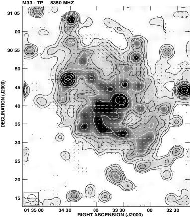
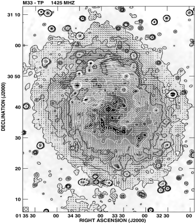
Figure 1.— Radio continuum emission from M33 at $\lambda=3.6$ cm (left) and $\lambda=20$ cm (right), with apparent B-vectors of polarized intensity superimposed. The beam areas are shown in the left corner of each figure. Contour levels are 0.5, 1, 2, 3, 4, 8, 16, 32 and 64 mJy/beam for the $3.6$ cm and 0.3, 0.6, 0.9, 1.2, 1.8, 2.4, 3.6, 4.8, 9.6 and 19.2 mJy/beam at $20$ cm Tabatabaei et al. 2007b .

In Borriello et al., 2009, some of the authors of the present paper have developed a semianalytical approach to compute the synchrotron emission from the Milky Way (MW) WIMP pairs annihilation. The comparison of the theoretical DM radio signal from our Galaxy with the observed emission, (where only the CMB is modelled and removed) allows to draw an exclusion plot in the $m_{\chi}$–$\left\langle\sigma_{\text{A}}v\right\rangle$ plane. For this purpose one can use the code described in de Oliveira Costa et al., 2008 where most of the whole sky radio observations in the range 10 MHz-100 GHz are collected and a scheme is described to derive interpolated, CMB cleaned sky maps at any frequency in this range. This result, however, is strongly affected by two problems:

• The difficulties in removing the foreground contribution from the radio continuum. Such a removal would allow, at least, an important refinement of the $m_{\chi}$–$\left\langle\sigma_{\text{A}}v\right\rangle$ bounds or, even better, the detection of DM. Let us recall that different approaches to the foreground removal at the WMAP frequencies produced very different results, exhibiting a residual signal (which has been interpreted as a signature of the DM annihilation) as in Finkbeiner, 2004 and Hooper at al., 2007 or no additional feature, as in a more recent analysis performed by the WMAP team itself Gold et al. (2008).

• The fact that the measured quantities are averaged by the integration along the line of sight which prevents a proper estimate of the local values of both galactic magnetic field and radio continuum emission. The high level of uncertainty on the local values of the MW magnetic field propagates on the results after the integration along the line of sight (an order ten kpc long path) is performed.

To overcome problems ii) we will reapply such an analysis to the nearby, close to face–on, $Scd$ galaxy Messier 33 (M33), taking advantage of the thinness of the region source of the signal. This galaxy is the third largest in the Local Group and is located at a distance of $840$ kpc from us Freedman et al. (1991). It has been extensively studied at all wavelengths: radio continuum (Tabatabaei et al. 2007b, , Tabatabaei et al. 2007c, , Tabatabaei et al., 2008), far infrared Tabatabaei et al. 2007a , near IR Cioni et al. (2007), optical Massey et al. (2006), UV (Ciani et al., 1984, Gordon et al., 1999), and X–ray Haberl & Pietsch (2001). Its kinematics has also been the subject of many studies Carignan (2006). M33 has an inclination of $\sim 56^{\circ}$ and due to its rather flocculent nature, it presents well defined arm and interarm regions. Some of the latter regions can be characterized by a particularly low level of radio emissivity (hereafter denoted for simplicity Radio Cavities), even though placed not far from the galactic center, and thus where possibly a non negligible magnetic field is at work. Hence, the poor radio emission would be simply due to a lack of astrophysical electrons/positrons. In this framework, the presence of a halo of WIMPs would inject in any case a flux of electron/positrons. These particles, while diffusing in the galaxy and propagating in the magnetic field, have to produce a radio signal compatible with the observed one. The requirement that the DM induced radio signal coming from a particular Radio Cavity of M33 does not overcome the observed one straightforwardly fixes bounds in the $m_{\chi}$–$\left\langle\sigma_{\text{A}}v\right\rangle$ plane.

Analyses devoted to the study of radio emission by external galaxies are already present in literature (see for example Tasitsiomi et al., 2003 and Colafrancesco, 2006), even if not focussing on Radio Cavities. It is worth noticing that the main advantage of considering a small region rather than the whole galaxy is that this approach allows to keep the different astrophysical hypothesis much more under control. For the purposes of the present work, M33 provides an ideal case since it is near, it has a small bulge–to–disk ratio, and therefore, it is possible to trace the inter–arm regions also relatively close to the central and densest regions. Moreover, due to its relatively small inclination (e.g. compared to M31), it allows to minimize the effects of the integration of the signal along the line of sight.

Unfortunately we cannot solve the first problem. The radio emission of galaxies like M33 has three components: the clumpy thin disk ($\sim 200$ pc scale height) with thermal and synchrotron emission from star-forming regions and supernova remnants, the smooth thick disk ($\sim 1$ kpc) with mostly synchrotron emission by young electrons originating from the thin disk, and the smooth halo (unknown extent) with synchrotron emission by old electrons from the thin disk. The relative contributions may vary from galaxy to galaxy, but in general the radio from the thick disk dominates, as visible in edge-on galaxies Beck (2009). The emission from the dark matter halo will mix with the thick disk emission but the mixing ratio is of course unknown. For this reason we preferred a conservative approach not subtracting any possible astrophysical component.

The paper is organized as follows. In Section 2 we describe the main characteristics of M33 Radio Cavity, whereas in Section 3 we compute the expected radio signal coming from it. Finally, in Sec. 4 we derive our constraints for WIMPs in the $m_{\chi}$–$\left\langle\sigma_{\text{A}}v\right\rangle$ plane and give our conclusions.

2. The radio cavity in M33

In the present analysis, we use the observations of M33 at $\lambda=3.6$ cm and $\lambda=20$ cm described in Tabatabaei et al. 2007b, and reported in Fig. 1.

A detailed description of the data acquisition reduction and analysis can be found in the above quoted reference. Here we shall just point out a few relevant facts. The data at $\lambda=3.6$ cm were obtained using the 100-m Effelsberg radiotelescope and the final map has a HPBW of $80^{\prime\prime}$ and an r.m.s noise of $\sim 220\,\mu$Jy/beam. On the other hand the data at $\lambda=20$ cm were obtained using the VLA-D array and corrected for lack of flux, due to missing short spacing, using single dish 20 cm observations obtained at the Effelsberg radiotelescope. The resulting map has an HPBW of $51^{\prime\prime}$ and an r.m.s noise of $\sim 70\,\mu$Jy/beam.

For the purpose of this work, the most noticeable feature, marked as a circle in Fig. 2, is the interarm cavity located at RA $\simeq 1^{{\rm h}}$33^m24.0^s and Dec $\simeq 30^{\circ}\ 35^{\prime}\ 39.0^{\prime\prime}$, i.e. at $\simeq 0.14^{\circ}$ SE of the bright nucleus (2.1 kpc from the center). This cavity has an area of $\sim 5\times 10^{3}$ arcsec², and is therefore well resolved at all wavelengths.

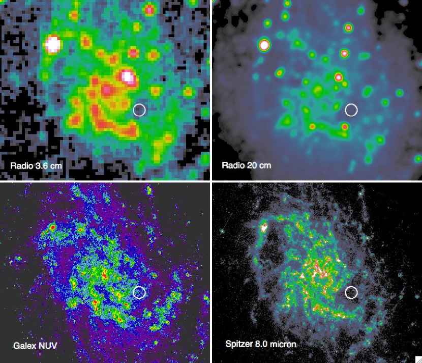
Figure 2.— Emission from M33 at different wavelengths. From the upper left clockwise: radio continuum at 3.6 cm, radio continuum at 20 cm, far infrared at 8.0 $\mu m$ (data from Spitzer telescope), and Near UV at 2300 Å. The Radio Cavity is marked by a circle.

Despite the small optical and radio flux coming from the cavity, there is no reason to believe the magnetic field there to be significantly smaller than the one in the surrounding regions. Therefore, the cavity is the ideal place to look for a DM signal, since there the ratio between the DM radio signal and the astrophysical foreground reaches its maximum value.

3. DM synchrotron signal

Let us first assume that M33 is perfectly face–on (later we will correct for the angle it forms with the line of sight) and consider a cartesian galactocentric coordinate system $(x,y,z)$ with the $z$–axis pointing in our direction. If $j_{\nu}$ is the synchrotron emissivity due to DM annihilation, the radio flux coming from an elementary volume $dV$ within M33 is given by $dI_{\nu}=j_{\nu}dV/4\pi D^{2}$, where $D$ is the distance of M33 from us.

Thanks to the face–on approximation and the large value of $D$, we can simply write $dV=D^{2}d\Omega dz$ and consider the integration along the line of sight as a simple integration along the $z$–axis. At last, the thinness of the integration volume allows us to take into account the angle $\theta$ the galaxy forms with the line of sight by simply multiplying the flux by $\cos{\theta}$. The result is

$$\frac{dI_{\nu}}{d\Omega}(\alpha,\beta)=\frac{\cos{\theta}}{4\pi}\int j_{\nu}(x,y,z)dz\ ,$$ (1)

where $\alpha=(x/D)\cos\theta$ and $\beta=y/D$ are two visual angles and where we chose the $y$–axis to be coincident with the M33 major axis.

We perform the integration of Eq. 1 over the range $z\in[-2\,\textrm{kpc},2\,\textrm{kpc}]$. This choice does not sensibly affect the results due to the exponential decrease of the DM synchrotron emissivity away from the galactic disk.

An analytical expression of $j_{\nu}$ can be found in Borriello et al., 2009 in terms of the DM density profile, the magnetic field and the interstellar radiation field (ISRF). The remaining parts of this section are therefore devoted to the parametrization of the Radio Cavity in M33.

3.1. Dark Matter density profile

It is not yet possible to uniquely determine the DM density of M33, nonetheless both a cored and a spiked profile can be deduced fitting the galaxy rotation curve (see Fig. 5 of Corbelli, 2003). The cored case is well represented by a Burkert Burkert (1995) density profile

$$\rho(r)=\left(1+\frac{r}{r_{0}}\right)^{-1}\left[1+\left(\frac{r}{r_{0}}\right)^{2}\right]^{-1}\rho_{0}\ ,$$

while the spiked profile is well described by and a NFW density distribution Navarro et al. (1996)

$$\rho(r)=\left(\frac{r}{r_{0}}\right)^{-1}\left(1+\frac{r}{r_{0}}\right)^{-2}\rho_{0}\ .$$

We consider two of the various fits obtained in Corbelli, 2003. Their defining parameters are:

model	$r_{0}$ (kpc)	$\rho_{0}$ (GeV $c^{-2}$ cm-3)
NFW	35	0.0574
Burkert	12	0.420

Profiles with a central slope steeper than $r^{-1}$ like the Moore profile Moore et al. (1999) are excluded Corbelli (2003).

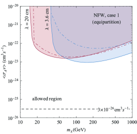
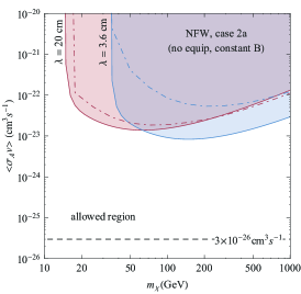
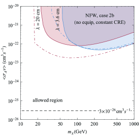
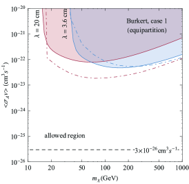
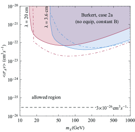
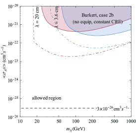
Figure 3.— Constraints in the $m_{\chi}$–$\left\langle\sigma_{A}v\right\rangle$ plane from radio observation of the Radio Cavity of M33 at 3.6 and 20 cm. Full annihilation into $b\bar{b}$ couples is assumed. The upper panels refers to a NFW DM density profile, the lower ones to a Burkert profile. Three cases are considered: (1) the equipartition hypotesis is verified; (2a) it is not and $B$ is constant across the cavity; (2b) it is not and CRE density is constant across the cavity. Solid lines refer to M33, while dot–dashed lines show the bounds obtainable – under the same physical hypothesis – for the MW (as in Borriello et al. (2009)).

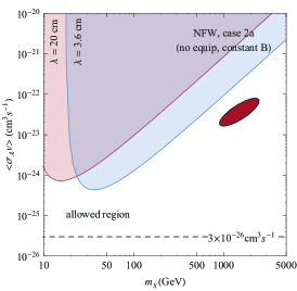
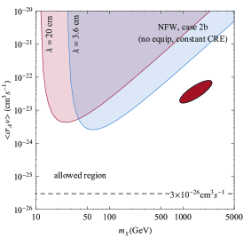
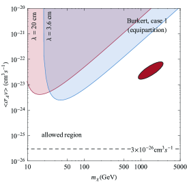
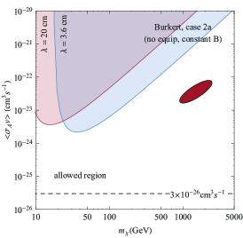
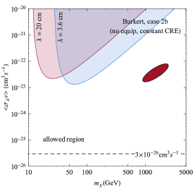
Figure 4.— As in Fig. 3 but for DM particles fully annihilating into $\mu^{+}\mu^{-}$ couples. This time the benchmark case is represented by the Pamela/Fermi LAT/Hess favored region (as in Meade et al., 2009) corresponding to the elliptical spot centered at about $10^{3}$ GeV and $10^{-23}$ cm³s^-1.

3.2. Magnetic Field

Following Tabatabaei et al., 2008, the equipartition total magnetic field strength in the radio cavity is estimated as $7.1\pm 0.5\ \mu$G. An exponential decrease is assumed to describe the field along the $z$ axis:

$$B=B_{0}\,e^{-|z|/z_{0}},$$ (2)

where $z_{0}$ is the scale height of the magnetic field. Observations of edge-on galaxies give a scale height of about 1.8 kpc for the synchrotron emission (see Beck, 2009). This leads to a magnetic field scale height of $z_{0}\sim\,7$ kpc, assuming a nonthermal spectral index of $\sim\,1$ (see e.g. Klein et al., 1982).

In the case in which the equipartition hypothesis were not valid the situation would be more involved and two cases can be taken into account:

(a) If the field strength is constant across the cavity, the cosmic ray electrons (CRE) have to be deficient to explain the low radio emission. $B$ can hardly be constant with height, too, but it could decrease even slower than with a scaleheight of 7 kpc if CREs suffer from strong energy losses (which is probable). We estimated a 7.5 $\mu$G field strength in this case and a scaleheight that could vary from 5 to 10 kpc;

(b) If however the CRE density is about constant across the cavity, the field there would be smaller than 7 $\mu$G and, if it is also constant with height, the $B$–scaleheight would be 2 times smaller. We estimated $B\sim 3.2\,\mu$G and $z_{0}=3.5$ kpc. This is however quite unlikely because CREs loose energy with height.

3.3. Interstellar Radiation Field

Once the high electrons are injected, they lose energy due, mainly, to two physical process: the synchrotron radiation we are interested in, and inverse Compton scattering off of the ISRF photons. Therefore, we need to characterize the ISRF in the cavity to properly subtract the amount of energy lost in the scattering with the photons.

According to Deul, 1989 we assume for the ISRF in the disk of M33 $U_{rad}^{(D)}(R)=5.32\,e^{-R/2.10}\,\chi,$ where $\chi=0.539$ eV cm^-3 is the MW’s ISRF at the Solar System position Weingartner & Draine (2001). The previous expression is obtained by setting the ISRF equal to $\chi$ to a galactocentric radius of $3.5$ kpc. To deduce the scale height of the exponential decrease of the ISRF far from the disk, we rescale the MW field in the same way. A galactocentric distance of $2.11$ kpc in M33 corresponds to $5.12$ kpc in the MW. Using the model described in Porter & Strong, 2005 it is possible to deduce that the MW’s ISRF scale height at a radius of $5.12$ kpc is equal to $3.72$ kpc which, when rescaled to M33, gives $1.53$ kpc.

Putting things together we parameterize the ISRF in the Radio Cavity as:

$$U_{rad}(z)=U_{0}\,e^{-|z|/h_{0}}\ ,$$

with $U_{0}=1.05$ eV cm^-3, and $h_{0}=1.53$ kpc.

4. Results and Conclusions

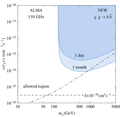
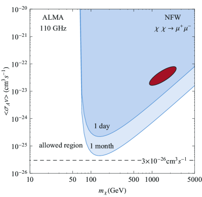
Figure 5.— Exclusion plots corresponding to a null detection (within the experimental sensitivity) radio flux. The left panel refers to DM particles annihilating into $b\,\bar{b}$ quarks derived for one day and one month of observation. The dot-dashed line represents the forecast (at 5$\sigma$) for five years of Fermi LAT data taking obtained by means of Galprop for optimized parameters (see Baltz et al., 2008 for details). The right panel refers instead to annihilation into $\mu^{+}\mu^{-}$. The exclusion regions are superimposed to the ellipse favored by Pamela/Fermi LAT/Hess data (see Meade et al., 2009).

Following the approach described above one can compute the expected radio emission due to electrons/positrons produced in the annihilation in pairs of WIMPs forming the halo of M33, and in particular the signal coming from the Radio Cavity which cannot overcome the observed signal. Hence, by using the observations of M33 at $\lambda=3.6$ cm and $\lambda=20$ cm, we obtained the exclusion plots reported in Fig. 3 and 4. Three cases are plotted for each wavelength and DM density profile: The equipartition hypothesis is verified (case 1: $B=7.1\,\mu$G, $z_{0}=7.0\,$kpc); The equipartition hypothesis is not verified and the field strength is constant across the cavity (case 2a: $B=7.5\,\mu$G, $z_{0}=10\,$kpc) or the CRE density is constant (case 2b: $B=3.2\,\mu$G, $z_{0}=3.5\,$kpc). Let us first consider the results shown in Fig. 3. For both wavelengths the bounds are compared to those corresponding to the MW (dot–dashed lines), derived in the same particle physics hypothesis Borriello et al. (2009) in which DM particles fully annihilate into $b\bar{b}$ couples. The results are quite dependent on the DM profile chosen, due to the position of the radio cavity (quite near the galactic center). In fact, assuming a Burkert density profile one gets less constraining results. In fact, at $2.1$ kpc from the galaxy center the Burkert profile is about $2/5$ of the NFW one, therefore we obtain six times weaker bounds from the cored case.

It is quite encouraging to observe that, at least for a favored case of an equipartition magnetic field and for a NFW profile, this calculation provides comparable or stringent bounds on DM than the ones obtained from our Galaxy. Moreover the M33 radio data used were not tailored for this aim, and thus could be largely improved in terms of resolution (see below).

Let us consider the case of very heavy WIMP directly annihilating into charged leptons as recently proposed in order to explain the positron excess observed by Pamela satellite Adriani et al. (2009) and the $e^{+}$-$e^{-}$ excess seen by Fermi LAT Abdo et al. (2008). This unexpected flux is made of electrons with energy greater that $\sim 100$ GeV. The synchrotron emission due to electrons of this energy is peaked around 100 GHz, quite far from the values we are considering here. Fig. 4 shows the bounds for the case in which the DM particle fully annihilate into $\mu^{+}\mu^{-}$ couples. In this case the DM contributes only for $\sim$ 1 % to the observed flux at 20 cm, while the situation improves at 3.6 cm, where the DM accounts for a order 10 % of the emission. Therefore, higher frequency observations would be needed to adequately consider this case.

Among ground-based telescopes, highest resolution (0.03$\arcsec$) and sensitivity (0.060 mJy) observations at high-frequencies ($\nu\sim$ 100 GHz) will be achieved by the Atacama Large Millimeter Array (ALMA). In addition Rotation Measurements Synthesis Heald et al. (2000) at as many wave wavelengths as possible will lead to a more precise magnetic field study, hopefully removing the degeneracy of possibilities shown in Fig. 3 and 4. Such a high angular resolution could improve our results. In fact if one can identify a small region inside the cavity from which one detects a vanishing flux (within the experimental sensitivity) this naturally results in a significant improvement of our bounds. To be quantitative let us consider ALMA observing at a 110 GHz in a compact configuration (50 antennas, 3.7 arcsec beam, 16 GHz bandwith). By using the ALMA Sensitivity Calculator, one gets a 0.01 mK surface brightness sensitivity for one day of exposure time.

In Fig. 5 we report the exclusion plots corresponding to the above null detection assumption for a NFW DM density profile. The left panel shows the results obtained for annihilation into $b\,\bar{b}$ while the right one refers to $\mu^{+}\mu^{-}$. For the hadronic case we compare our bounds, derived for one day and one month of observation, with the forecast (at 5$\sigma$) corresponding to five years of Fermi LAT data taking Baltz et al., 2008. Interestingly radio observations perform better for heavy WIMPs. In the right panel our exclusion regions are superimposed to the ellipse favored by Pamela/Fermi LAT/Hess data (see Meade et al., 2009 and references therein).

To summarize, we derived the expected secondary radiation due to synchrotron emission from high energy electrons/positrons produced in DM annihilations in M33. The comparison of the expected DM induced emission with radio continuum observations, especially focussed on a particular low emitting Radio Cavity, allows to obtain bounds in the $m_{\chi}$–$\left\langle\sigma_{\text{A}}v\right\rangle$ plane. By using not tailored archival data we are able to put bounds comparable with ones obtainable by full sky observations of the radio emission from our Galaxy. This suggests the possibility that focused observations of small and well known astrophysical object could gain a great predictive power. To be more quantitative on the potentiality of the method we have considered an optimistic scenario were a high resolution radio telescope like ALMA does not detect any flux (within the experimental sensitivity) in a region inside the radio cavity. In this case the bounds we can derive on WIMPs parameters are better than the corresponding Fermi LAT forecast in the case of heavy WIMPs decaying into hadrons. Assuming instead annihilation into muons we could be able to rule out the region favored by Pamela/Fermi LAT/Hess in a single day of observation.

References

- Abdo et al. (2008) Abdo, A. A. et al. 2009, Phys. Rev. Lett., 102, 181101
- Adriani et al. (2009) Adriani, O. et al. 2009, Phys. Rev. Lett. 102, 051101
-
(3)
ALMA Sensitivity Calculator,
http://www.eso.org/sci/facilities/alma/observing/tools/etc/ - Aloisio et al. (2004) Aloisio, R., Blasi, P., & Olinto, A.V. 2004, JCAP, 0405, 007
- Baltz & Edsjo (1998) Baltz, E. A., & Edsjo, J. 1999, Phys. Rev. D, 59, 023511
- Baltz & Wai (2004) Baltz, E. A., & Wai, L. 2004, Phys. Rev. D, 70, 023512
- Baltz et al. (2008) Baltz, E. A. et al. 2008, JCAP, 0807, 013
- Beck (2009) Beck, R. 2009, Ap&SS, 320, 77
- Bergstrom (2000) Bergstrom, L. 2000, Rept. Prog. Phys., 63, 793
- Bergstrom et al. (2006) Bergstrom, L., Fairbairn, M., & Pieri, L. 2006, Phys. Rev. D, 74, 123515
- Bertone et al. (2005) Bertone, G., Hooper, D., & Silk, J. 2005, Phys. Rept., 405, 279
- Blasi et al. (2002) Blasi, P., Olinto, A. V., & Tyler, C. 2003, Astropart. Phys., 18, 649
- Borriello et al. (2009) Borriello, E., Cuoco, A., & Miele, G. 2009, Phys. Rev. D, 79, 023518
- Burkert (1995) Burkert, A. 1995, ApJ, 447, L25
- Carignan (2006) Carignan, C., Chemin, L., Huchtmeier, W. K., & Lockman, F. J. 2006, ApJ, 641, L109
- Ciani et al. (1984) Ciani, A., D’Odorico, S., Benvenuti, P. 1984, A&A, 137, 223
- Cioni et al. (2007) Cioni, M.-R. L. et al., arXiv:0709.2949
- Colafrancesco (2005) Colafrancesco, S., Profumo, S., & Ullio, P. 2006, A&A, 455, 21
- Colafrancesco (2006) Colafrancesco, S., Profumo, S., & Ullio, P. 2007, Phys. Rev. D, 75, 023513
- Corbelli (2003) Corbelli, E. 2003, MNRAS, 342, 199
- de Oliveira Costa et al. (2008) de Oliveira-Costa, A., Tegmark, M., Gaensler, B. M., Jonas, J., Landecker, T. L., & Reich, P. 2008, MNRAS, 388, 247
- Deul (1989) Deul, E. R. 1989, A&A, 218, 78
- Donato et al. (2003) Donato, F., Fornengo, N., Maurin, D., Salati P., & Taillet, R. 2004, Phys. Rev. D, 69, 063501
- Finkbeiner (2004) Finkbeiner, D. P. 2004, arXiv:astro-ph/0409027
- Freedman et al. (1991) Freedman, W. L., Wilson, C. D., & Madore, B. F. 1991, ApJ, 372, 455.
- Gold et al. (2008) Gold, B., et al. 2009, ApJS, 180, 265
- Gordon et al. (1999) Gordon, K. D., Hanson, M. M., Clayton, G. C., Rieke, G. H., & Misselt, K. A. 1999, ApJ, 519, 165
- Haberl & Pietsch (2001) Haberl, F., & Pietsch, W. 2001, A&A, 373, 438
- Heald et al. (2000) (Heald, G. et al. 2000, A&A 503, 409)
- Hooper & Silk (2004) Hooper, D., & Silk, J. 2005, Phys. Rev. D, 71, 083503
- Hooper at al. (2007) Hooper, D., Finkbeiner, D. P., & Dobler, G., 2007, Phys. Rev. D, 76, 083012
- Jeltema & Profumo (2008) Jeltema, T. E., & Profumo, S. 2008, ApJ, 686, 1045
- Jungman et al. (1995) Jungman, G., Kamionkowski, M., & Griest, K. 1996, Phys. Rept., 267, 195
- Klein et al. (1982) Klein, U., Beck, R., Buczilowski, U. R., & Wielebinski, R. 1982, A&A, 108, 176
- Komatsu et al. (2008) Komatsu, E., et al. 2009, APJS, 180, 330
- Massey et al. (2006) Massey, P., Olsen, K. A. G., Hodge, P. W., Strong, S. B., Jacoby, G. H., Schlingman, W., & Smith, R. C. 2006, AJ, 131, 2478
- Meade et al. (2009) Meade, P., Papucci, M., Strumia, A., & Volansky, T. 2009, arXiv:0905.0480 [hep-ph].
- Moore et al. (1999) Moore, B., Ghigna, S., Governato, F., Lake, G., Quinn, T. R., Stadel, J. & Tozzi P. 1999, ApJ., 524, L19
- Navarro et al. (1996) Navarro, J. F., Frenk, C.S., & White, S. D. M. 1997, ApJ, 490, 493
- Porter & Strong (2005) Porter, T. A., & Strong, A. W. 2005, astro-ph/0507119
- Regis & Ullio (2008) Regis, M., & Ullio, P. 2008, Phys. Rev. D, 78, 043505
- (42) Tabatabaei, F. S., et al. 2007, A&A, 466, 509
- (43) Tabatabaei, F. S., Krause, M., & Beck, R. 2007, A&A, 472, 785
- (44) Tabatabaei, F. S., Beck, R., Krügel, E., Krause, M., Berkhuijsen, E. M., Gordon, K. D. & Menten, K. M. 2007, A&A, 475, 133
- Tabatabaei et al. (2008) Tabatabaei, F. S., Krause, M., Fletcher, A., & Beck, R. 2008, A&A, 490, 1005
- Tasitsiomi et al. (2003) Tasitsiomi, A., Siegal-Gaskins, J. M., & Olinto, A. V. 2004, Astropart. Phys., 21, 637
- Weingartner & Draine (2001) Weingartner, J. C., & Draine, B. T. 2001, ApJ, 134, 263
- Zhang & Sigl (2008) Zhang, L., & Sigl, G. 2008, JCAP 09, 027