A Near-Infrared Spectroscopic Survey of K-selected Galaxies at $z$ $\sim$ 2.3: Comparison of stellar population synthesis codes and constraints from the rest-frame NIR

Abstract

We present SED modeling of a sample of 34 K-selected galaxies at $z\sim$ 2.3. These galaxies have NIR spectroscopy that samples the rest-frame Balmer/4000Å break as well as deep photometry in thirteen broadband filters. New to our analysis is IRAC data that extend the SEDs into the rest-frame NIR. Comparing parameters determined from SED fits with and without the IRAC data we find that the IRAC photometry significantly improves the confidence intervals of $\tau$, A_v, M${}_{\mbox{\scriptsize star}}$, and SFR for individual galaxies, but does not systematically alter the mean parameters of the sample. We use the IRAC data to assess how well current stellar population synthesis codes describe the rest-frame NIR SEDs of young galaxies where discrepancies between treatments of the TP-AGB phase of stellar evolution are most pronounced. The models of Bruzual & Charlot (2003), Maraston (2005), and Charlot & Bruzual (2008) all successfully reproduce the SEDs of our galaxies with $\leq$ 5% differences in the quality of fit; however, the best-fit masses from each code differ systematically by as much as a factor of 1.5, and other parameters vary more, up to factors of 2-3. A comparison of best-fit stellar population parameters from different SPS codes, dust laws, and metallicities shows that the choice of SPS code is the largest systematic uncertainty in most parameters, and that systematic uncertainties are typically larger than the formal random uncertainties. The SED fitting confirms our previous result that galaxies with strongly suppressed star formation account for $\sim$ 50% of the K-bright population at $z\sim$ 2.3; however, the uncertainty in this fraction is large due to systematic differences in the SSFRs derived from the three SPS models.

1. Introduction

The observed flux from a galaxy as a function of wavelength or frequency, its spectral energy distribution (SED), represents the integrated light of its stellar populations and is a valuable tool for determining properties such as its age, and current mass contained in stars. Interpreting observations of galaxy SEDs requires creating synthetic spectra using our best understanding of stellar spectra, stellar evolution, and dust absorption. This process, known as stellar population synthesis (SPS) was first implemented by Tinsley (1967, 1972) and has subsequently been refined into increasingly sophisticated models (e.g., Bruzual 1983; Renzini & Buzzoni 1986; Bruzual & Charlot 1993; Worthey 1994; Fioc & Rocca-Volmerange 1997; Leitherer et al. 1999; Bruzual & Charlot 2003; Maraston 2005; Bruzual 2007; Conroy et al. 2008).
With the advent of deep multiwavelength extragalactic surveys and the refinement of photometric redshift techniques, large, statistically complete samples of galaxies with broadband SEDs are now available for studying the evolution of galaxy properties in a systematic way up to $z\sim$ 2-3 (e.g., Förster Schreiber et al. 2004; Labbé et al. 2005; van Dokkum et al. 2006; Papovich et al. 2006; Fontana et al. 2006; Daddi et al. 2007; Wuyts et al. 2007; Pérez-González et al. 2008; Drory & Alvarez 2008; Marchesini et al. 2008, and many others). The demand for SPS codes that provide accurate synthetic SEDs for a given parameter set is now greater than ever as they are $the$ tool for extracting astrophysical information from these data.
Using the current generation of SPS models these studies have shown that a large fraction of the stellar mass (M${}_{\mbox{\scriptsize star}}$) in massive galaxies is assembled by $z\sim$ 2 (e.g., Fontana et al. 2006; Pérez-González et al. 2008; Marchesini et al. 2008), and that a significant fraction of these galaxies are already passively evolving (e.g., Labbé et al. 2005; Papovich et al. 2006; Kriek et al. 2006). Unfortunately, the current SPS models do have significant challenges to overcome (see e.g., Conroy et al. 2008), making it unclear how robust some of these results are (see e.g., the discussion in Marchesini et al. 2008). Furthermore, it is well known that stellar population parameters derived from fitting broadband SEDs suffer from systematic uncertainties caused by the fact that metallicity, the initial mass function (IMF), and dust extinction law cannot be constrained by broadband SEDs alone. Instead, these parameters must be assumed a priori when creating the set of synthetic SEDs used in the fitting. More recently it has become clear that the treatment of SPS itself (e.g., the choice of isochrones, stellar libraries, and integration method) can result in synthetic spectra that look strikingly different for a similar set of input parameters (e.g., Maraston 2005, Maraston et al. 2006; Bruzual 2007; Conroy et al. 2008) and that the choice of SPS method is now an additional systematic error in the interpretation of galaxy SEDs.
One of the major challenges for SPS remains to be a complete treatment of the thermally-pulsating asymptotic giant branch (TP-AGB) stars. This population of stars are notoriously challenging to model because they have complex physics such as thermal pulses, evolving chemical compositions, rapid mass-loss rates, and self-obscuring dust shells (see e.g., Marigo et al. 2008, and references therein). Furthermore, their lifetimes are short which means they are rarely found in clusters and therefore the majority of empirical spectra come from field stars of unknown metallicity (e.g., Lançon & Wood 2000, Lançon & Mouchine 2002). Nevertheless, they cannot be ignored in SPS because they are bright in the rest-frame NIR and can dominate the total NIR luminosity of young stellar populations with ages between 0.2 to 2.0 Gyr (e.g., Maraston 2005, Bruzual 2007). The treatment of TP-AGB stars in SPS modeling is now a key issue in the study of stellar masses, because the rest-frame NIR also traces a galaxy’s old stellar population and therefore represents its integrated star formation history (SFH). If galaxies undergo multiple bursts of star formation (SF) at widely spaced epochs, the rest-frame NIR becomes the critical wavelength range for determining stellar masses. For young galaxies at high redshift, SPS codes with different treatments of TP-AGB evolution can produce stellar masses and ages that systematically differ by roughly a factor of 2 for identical SEDs (e.g., Maraston et al. 2006; Kannappan & Gawiser 2007; Wuyts et al. 2007; Bruzual 2007). Indeed, based on discrepancies between kinematically-derived, and photometrically-derived stellar masses of galaxies at $z\sim$ 1, van der Wel et al. (2006) have even argued that the stellar masses of young, early-type galaxies are better determined by SED fits that exclude the rest-frame NIR.
Recent papers by Maraston et al. (2006) and Bruzual (2007) have suggested that $Spitzer$ observations could be important for resolving some of the differences between SPS codes, particularly the TP-AGB treatment. IRAC observes at 3.6$\micron$, 4.5$\micron$, 5.8$\micron$ and 8.0$\micron$, effectively the rest-frame NIR of galaxies at $z\sim$ 2. At this redshift the universe is young, $\sim$ 3 Gyr, and therefore the majority of observed galaxies contain the young stellar populations that should be dominated by TP-AGB stars; however, they have not yet acquired an underlying old stellar population that must be accounted for when studying TP-AGB effects in the rest-frame NIR in low redshift galaxies (e.g., Riffel et al. 2008). Using a sample of 7 galaxies at 1.4 $<z<$ 2.7 from the GOODS survey, Maraston et al. (2006) have argued that their models produce better fits to young galaxies than the Bruzual & Charlot (2003, hereafter BC03) models and this is caused by their empirically calibrated fuel consumption treatment of the TP-AGB phase. Using the next generation of the BC03 code that includes improved evolutionary tracks for TP-AGB stars from Marigo et al. (2008), Bruzual (2007) have fit the same 7 galaxies and showed that they now obtain parameters closer to those in Maraston et al. (2006).
In Kriek et al. (2006; 2007; 2008a, hereafter K08) we presented SED modeling of a sample of 36 K-selected galaxies at $z\sim$ 2.3 that was based on extensive NIR spectroscopy covering the JHK bands obtained from GNIRS on Gemini, as well as broadband photometry. These data constrain the galaxy’s SEDs from the rest-frame UV to optical and K08 compared fits with and without the NIR spectroscopy to determine how parameters determined from fitting broadband data alone compare with those determined with the higher resolution spectroscopy and spectroscopic redshifts. Recently, we have obtained IRAC observations of this sample and this allows us to extend the SED modeling into the rest-frame NIR. With deep photometry in 13 broadband filters (UBVRIz^′JHK+IRAC) as well as high-resolution NIR spectroscopy that covers the rest-frame Balmer/4000Å break, this sample of galaxies are likely to have the best-constrained SEDs of young massive galaxies at $z\sim$ 2.3 until more powerful optical and mid-infrared spectroscopic capabilities become available from ground-based 20-30m telescopes and JWST, respectively.
In this paper we explore how well the properties of these galaxies can be derived from their SEDs, with a focus on the rest-frame NIR. Specifically, we concentrate on four issues, 1) Improvement in Constraints and Systematic Errors: Does IRAC data improve the constraints on stellar population parameters for $z\sim$ 2.3 galaxies, or does it increase the uncertainties because the models fail to correctly reproduce the rest-frame NIR SED? Are there systematic errors in the stellar population parameters determined without the rest-frame NIR data? 2) Best-possible constraints: Ignoring systematic effects such as metallicity, dust law, IMF, and choice of SPS code, what are the best-possible constraints on the stellar population parameters of individual galaxies we can expect from their SEDs alone? 3) Comparison of SPS Codes: How well do the most-used SPS codes describe the SEDs of young stellar populations in the rest-frame NIR? Including the IRAC data, do any of the codes provide better fits to the data? What are the systematic differences in parameters for individual galaxies using various SPS codes, dust laws, and metallicities, and which of these effects is most significant? 4) Are passive galaxies really passive? Approximately 50% of the galaxies in our sample show no emission lines in their spectra. Do all of these galaxies have strongly suppressed star formation, or are some dusty star forming galaxies with enough dust to obscure the emission-line regions?
This paper is organized as follows. In $\S$ 2 we briefly review the observational data used in our analysis. In $\S$ 3 we introduce the SPS codes used in our fitting, and discuss our fitting and error estimation methods. In $\S$ 4 we evaluate the constraints on stellar population parameters when including the rest-frame NIR data. In $\S$ 5 we compare the quality of fits from the various SPS codes and compare the systematic changes in parameters from these codes. We assess the systematic effects from the various assumptions of dust law and metallicity compared to SPS code in $\S$ 6, and in $\S$ 7 we examine what fraction of the galaxies have strongly suppressed star formation based on their SEDs. We conclude with a summary in $\S$ 8
Throughout this paper we assume a $\Omega_{m}$ = 0.3, $\Omega_{\Lambda}$ = 0.7, H₀ = 70 km s^-1 Mpc^-1 cosmology.

2. Data

2.1. The Galaxy Sample

The 34 galaxies used in this study are those with NIR spectroscopic observations performed by Kriek et al. (2006; 2007), K08. Galaxies were selected for the sample based on their K-band magnitude (K $<$ 19.7, Vega magnitude) and that they were likely to lie in the 2.0 $<z<$ 2.7 redshift range based on their photometric redshift probability distribution as derived from broadband UBVRIz^′JHK photometry. As discussed in K08, Mann-Whitney and Kolmorov-Smirnov tests show that this sample is representative of the distribution of the $z_{\mbox{\scriptsize phot}}$, J-K, R-K, and (U-V)_rest colors of a mass-limited sample at 2 $<z<$ 3. It may be less representative of a K-bright subsample of the 2 $<z<$ 3 population because the overall K-bright population tends to have a lower median redshift and narrower redshift distribution than the spectroscopic sample (K08). Small biases like these should not affect the analysis in this paper. Approximately 20% (7/34) of the sample have spectroscopic redshifts 1.5 $<z<$ 2.0. These galaxies may not necessarily be representative of the stellar populations of a mass-limited sample in this redshift range; however, we include them in this analysis.

2.2. Photometric Data

The UBVRIz^′JHK photometry for galaxies in the fields SDSS1030, CW1255, HDFS1, and HDFS2, (hereafter, the MUSYC fields) is derived from the catalogues presented in Gawiser et al. (2006) and Quadri et al. (2007). Photometry in the same bands for galaxies in the ECDFS field are derived from the catalogues presented in Taylor et al. (2008). The IRAC photometry for galaxies in the MUSYC fields is presented in Marchesini et al. (2008) and we refer to that paper for a detailed discussion of the data reduction and catalogue creation. The IRAC data for the ECDFS field was obtained as part of the SIMPLE survey and is discussed in Damen et al. (2008). We have added a systematic error of 10% in quadrature to the IRAC photometric errors to account for zero point uncertainties and the color-dependent flat fielding errors.
A few of the galaxies in the K08 sample were located close to the edge, or completely out of the region covered by the IRAC data. SDSS1030-101 is missing 3.6$\micron$ and 5.8$\micron$ data, whereas SDSS1030-1839 is missing 4.5$\micron$ and 8.0$\micron$ data. These galaxies still have data in the complementary IRAC bands so we retain them in the sample. The galaxies SDSS1030-301 and SDSS1030-1813 were near the edge of the field and due to the dither pattern have only a few frames of data in the IRAC bands. Although they are detected, the lack of data make background subtraction and cosmic ray rejection difficult so we remove them from the sample. Removal of these galaxies reduces the sample to 34 of the 36 galaxies presented in K08.

2.3. NIR Spectroscopic Data

The reduction of the NIR spectroscopic data used in our SED modeling was discussed in detail in Kriek et al. (2006). Briefly, the data were obtained with the GNIRS instrument on Gemini-South using the 0.675^′′-wide slit and the 32 l/mm grating in cross-dispersed mode which provided a resolving power of R $\sim$ 1000. Spectroscopic redshifts were determined for 17/34 galaxies that had detected emission lines. For the remaining 17 galaxies that did not have detectable emission lines K08 determined a spectroscopic continuum redshift using SED modeling of the NIR spectra and broadband photometry. In this analysis we use the low-resolution binned spectra constructed by K08. Each data point in the binned spectra contains 80 good pixels from the observed spectrum, corresponding to $\sim$ 400Å observed frame. Absolute flux calibration of the spectra is performed using the broadband JHK magnitudes.

3. SED Fitting and Stellar Population Parameters

3.1. Stellar Population Models

At present, there are several well-tested SPS codes publically available. Codes such as PEGASE (Fioc & Rocca-Volmerage 1997), Bruzual & Charlot (2003, hereafter BC03), Maraston (2005, hereafter M05), Starburst99 (Vazquez & Leitherer 2005), and Charlot & Bruzual (2008, in preparation, hereafter CB08) all provide synthetic spectra for SED modeling.
As pointed out by M05, the PEGASE, Starburst99, and BC03 models use similar stellar spectral libraries, isochrones, and treatment of the TP-AGB phase of stellar evolution. Therefore, in our fitting we use the BC03 models assuming they are representative of this class. We also perform fits using the M05 code which uses the fuel consumption approach as an alternative to isochrone synthesis for modeling stellar evolution off the main sequence. Lastly, we perform fits with the CB08 code which is similar to the BC03 code except that it also includes updated evolutionary tracks for TP-AGB stars from Marigo et al. (2008). Taken together these three codes span the different treatments of TP-AGB stars currently available.

3.2. Fitting Method

The fitting procedure used in our analysis is analogous to the one outlined in Kriek et al. (2006) and K08. The photometric and spectroscopic data are fit to models with 34 exponentially declining SFHs (parameterized by $\tau$) ranging from 0.01 to 20.0 Gyr. We fit 45 different ages ($t$) ranging from 0.01 to 13 Gyr, but only allow those that are less than the age of the universe at the redshift of the galaxy. For the majority of comparisons in this paper we assume solar metallicity and a Calzetti et al. (2000) dust law as our “control” model. The V-band attenuation (A_v) is allowed to range between 0 and 4 mag in increments of 0.1. When fitting galaxies without emission lines we also adopt $z$ as a free parameter and fit in increments of $\delta$z = 0.01.
To maintain continuity with the fits presented in K08 we adopt a Salpeter (1955) IMF. Although it is widely accepted that the Kroupa (2001) and Charbrier (2003) IMFs are likely to be better choices for a universal IMF; we note that the galaxies in our sample are young and the main sequence turnoff mass is much larger than the mass at which these IMFs differ, therefore, the choice between these IMFs does not significantly affect the shape of the synthetic SEDs, only the normalization of the M${}_{\mbox{\scriptsize star}}$. Given an average age of $\sim$ 1 Gyr, the M${}_{\mbox{\scriptsize star}}$ computed for our sample can be converted to a Charbrier or Kroupa IMF simply by multiplying by scaling factors of 0.57 and 0.63, respectively. Our values of M${}_{\mbox{\scriptsize star}}$ are also corrected to account for gas recycled to the interstellar medium from supernovae and planetary nebula. Therefore, our M${}_{\mbox{\scriptsize star}}$ corresponds to living stars plus stellar remnants, but do not include recycled gas.
For each SPS SED, we find a normalization ($X$) by minimizing the function

$$\chi_{r}^{2}=\frac{1}{N_{DOF}}\sum_{i=1}^{N_{filters}}\frac{(X\cdot f_{model(\tau,t,A_{v},z),i}-f_{obs,i})^{2}}{\delta f_{obs,i}^{2}},$$ (1)

where $N_{DOF}$ is the number of degrees of freedom, f_obs,i is the observed flux in the $i^{th}$ filter, $\delta$f_obs,i is the error in the observed flux, and f${}_{model(\tau,t,A_{v},z),i}$ is the flux of model SED which is a function of $\tau$, $t$, A_v, and $z$. We then construct a $\chi_{r}^{2}$-surface as a function of the synthetic SPS model parameters $\tau$, $t$, A_v, and $z$. The best fit SPS model is determined by finding the location of the minimum on the $\chi_{r}^{2}$ surface.
The 1$\sigma$ confidence intervals in the model parameters are determined using the Monte Carlo method suggested by Papovich et al. (2001) and K08. In these simulations the photometric and spectroscopic data are perturbed randomly within their uncertainties and then the SPS models are fit again. From 200 simulations per galaxy we find the value of $\chi_{r}^{2}$ that encompasses the $\chi_{r}^{2}$ from 68% of the Monte Carlo simulations. Returning to the original $\chi_{r}^{2}$ fitting surface, locations with $\chi_{r}^{2}$ below this value are considered to be allowable within the 1$\sigma$ errors. The strength of this method is that by using the original $\chi_{r}^{2}$-surface the correlations between errors in the parameters are preserved.

4. Improvement in Stellar Population Parameters from Rest-Frame NIR Data

In this section we examine the importance of IRAC data for constraining the stellar population parameters of $z\sim$ 2.3 galaxies from their SEDs without considering systematic effects such as the choice of metallicity, dust law, IMF and SPS code. We test for potential systematic differences in parameters that result from fitting with and without constraints on the rest-frame NIR SED, as well as how much (if at all) the rest-frame NIR improves the uncertainties in the stellar population parameters. Throughout this section we use the BC03 $\tau$-models with solar metallicity, the Calzetti et al. (2000) dust law, and a Salpeter IMF as our “control” model for the comparisons.

4.1. Comparison of SED Fits With and Without IRAC Data

In Table 1 we list the best fit SED parameters and 1$\sigma$ uncertainties determined from fits to the UBVRIz^′ broadband data and NIR spectroscopy (i.e., without the IRAC data, hereafter we refer to this as U$\rightarrow$z^′+NIRspec), as well as those from fits with the UBVRIz^′, NIR spectroscopy and the IRAC data (hereafter U$\rightarrow$8$\micron$+NIRspec). Table 1 also contains the parameter $\langle t\rangle_{\mbox{\scriptsize SFR}}$, defined as the SFR-weighted mean age of the stellar population (see Förster Schreiber et al. 2004). The parameter $t$ in Table 1 is the time since the onset of SF; however, in $\tau$-models galaxies are continually forming stars and therefore $\langle t\rangle_{\mbox{\scriptsize SFR}}$  defines the mean age of the stellar population that dominates the light of the galaxy. Throughout this paper we use $\langle t\rangle_{\mbox{\scriptsize SFR}}$ as the metric of the age of the galaxies.
K08 also determined SED parameters for this sample of galaxies using the U$\rightarrow$z^′+NIRspec data (see their Table 2). Some of our U$\rightarrow$z^′+NIRspec fit parameters are identical to those determined by K08; however, most of the parameters and uncertainties have changed by small amounts. These minor differences occur for several reasons. Firstly, our grid of $\tau$ and $t$ is larger and the spacing is somewhat different than the K08 grid. Secondly, some of the broadband fluxes have changed slightly in our newer photometric catalogues. Thirdly, we use a new fitting code which finds the SED normalizations using a different algorithm than the K08 code. This leads to small numerical differences in the $\chi_{r}^{2}$’s. Frequently the difference between the minimum $\chi_{r}^{2}$ of the K08 best fit and our best fit is $<$ 0.1%; however, the best fit parameters can be significantly different. There are a few galaxies that have large differences in parameters; however, the 1$\sigma$ confidence intervals from our fits and the K08 fits still span the same range of values for these galaxies. Due to these changes we use the parameters and uncertainties for the U$\rightarrow$z^′+NIRspec data determined using our fitting code for consistency of comparison.
In Figures 1 and 2 we plot F_λ as a function of observed wavelength for the photometric data as well as the best fitting SEDs. Broadband photometry is plotted in red and the binned NIR spectroscopic data is plotted in cyan. The SEDs fit with the U$\rightarrow$z^′+NIRspec data are plotted in grey, and the SEDs fit with the U$\rightarrow$8$\micron$+NIRspec data are plotted in black. The fit parameters are listed in the panels of Figures 1 and 2 for ease of comparison. The broadband JHK fluxes have been plotted for reference, but were not used in the fitting.
Examination of Figures 1 and 2 shows that for $\sim$ 50% of the galaxies the SEDs fit without the IRAC photometry are still consistent with the IRAC photometry at $<$ 1$\sigma$. Comparing the best fit SED parameters we find that for 27/34 galaxies (79%) the $z$, $\tau$, $t$, A_v, M${}_{\mbox{\scriptsize star}}$, SFR, and $\langle t\rangle_{\mbox{\scriptsize SFR}}$ determined without IRAC data all agree with those fit with IRAC data within the 1 $\sigma$ confidence intervals. This demonstrates that for most galaxies any systematic changes in the fits that occur due to the inclusion of the IRAC data are smaller than the formal confidence intervals (we explore this in more detail in $\S$ 4.3). For the remaining 7/34 galaxies (1030-1531, 1030-2728, 1256-519, 1256-1967, HDFS2-509, ECDFS-6842, ECDFS-12514) there is a mixed range of agreement between the black and grey SEDs and the best fit parameters.
The largest difference in best fit parameters as well as SED shape is for the galaxy 1256-519, which provides a qualitative illustration of the importance of the rest-frame NIR photometry for constraining stellar population parameters. Without the IRAC data galaxy 1256-519 is best fit as a young, dusty star forming galaxy ($t$ = 0.3 Gyr, A_v = 3.2, SFR $\sim$ 400 M_⊙ yr^-1), but including the IRAC data it is best fit as an old, moderately-dusty quiescent galaxy ($t$ = 2.5 Gyr, A_v = 0.9, SFR $\sim$ 3 M_⊙ yr^-1). As Figure 1 illustrates, there is little difference between these two SEDs in the rest-frame optical; however, their fluxes in the rest-frame NIR are quite different. A young-and-dusty population is much brighter in the rest-frame NIR than an old-and-quiescent population. Once the IRAC data is included it is clear that the galaxy has an SED that is consistent with an old-and-quiescent population.
The importance of the rest-frame NIR for distinguishing young-and-dusty populations from old-and-quiescent populations has already been discussed by previous authors, e.g., Labbé et al. (2005), Papovich et al. (2006), Wuyts et al. (2007) and Williams et al. (2008). These studies have suggested that simple color-color diagrams could be an efficient method for separating these types. Galaxy 1256-519 clearly demonstrates how critical the rest-frame NIR is; even with spectroscopic redshifts and high-resolution spectrophotometry near the Balmer/4000Å break, it can still be difficult to robustly distinguish young-and-dusty from old-and-quiescent populations without additional data on the rest-frame NIR SED.

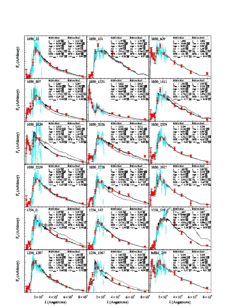
Figure 1.— SEDS fit using BC03 models without IRAC data (grey SED) and with IRAC data (black SED). The red points are the broadband photometry and the cyan points are the binned NIR spectroscopy.

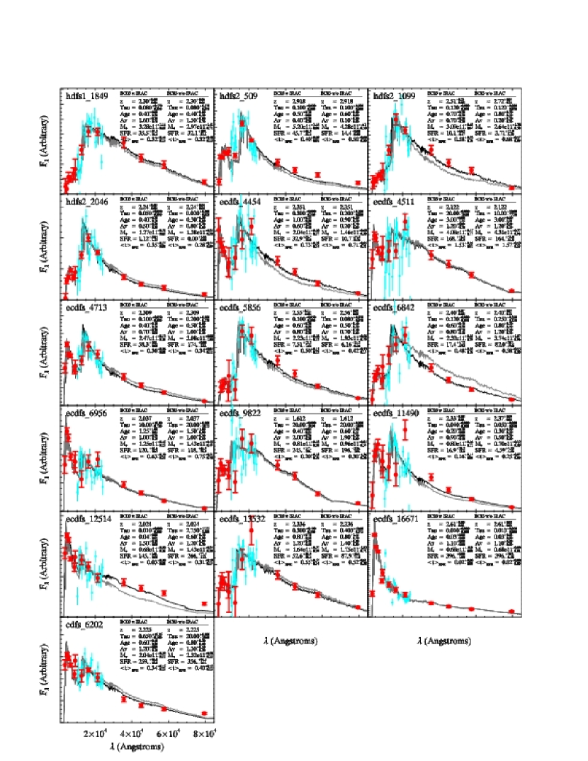
Figure 2.— As Figure 1.

4.2. Improvement in Photometric Redshifts with IRAC data

Accurate determination of the stellar population parameters of $z\sim$ 2 galaxies with broadband data requires high quality photometric redshifts ($z_{\mbox{\scriptsize phot}}$). Using this spectroscopic sample K08 showed that the $z_{\mbox{\scriptsize phot}}$’s determined using the Rudnick et al. (2001; 2003) code, which employs the Coleman et al. (1980) and Kinney et al. (1996) templates, were systematically overestimated by $\Delta z$/(1 + $z$) = 0.08, where $\Delta$$z$ = ($z_{\mbox{\scriptsize phot}}$ - $z_{\mbox{\scriptsize spec}}$), and had a scatter of 0.13 in the same units. Although random errors in $z_{\mbox{\scriptsize phot}}$ can be overcome with larger samples, systematic errors can pose significant problems, particularly when studying the evolution of the stellar mass density or luminosity density (see, e.g., K08, van Dokkum et al. 2006). It has been suggested by some authors that the 1.6$\micron$ bump feature present in the SEDs of evolved stellar populations could be a useful $z_{\mbox{\scriptsize phot}}$ indicator (e.g., Simpson & Eisenhardt 1999; Sawicki 2002). This feature falls in the IRAC bands for galaxies at 1.5 $<z<$ 3.0 and given the large scatter and systematic offset between the $z_{\mbox{\scriptsize phot}}$ and the spectroscopic redshifts ($z_{\mbox{\scriptsize spec}}$) seen by K08, it is worth investigating whether deep IRAC data might improve the $z_{\mbox{\scriptsize phot}}$ of $z\sim$ 2.3 galaxies. We test this by determining $z_{\mbox{\scriptsize phot}}$ using the broadband photometry with and without the IRAC data and comparing these to the $z_{\mbox{\scriptsize spec}}$.
The $z_{\mbox{\scriptsize phot}}$’s are computed using the EAZY photometric redshift code (Brammer et al. 2008). We use the standard EAZY v1.0 template set which is determined using nonnegative matrix factorization of SED models from the PÉGASE code (Fioc & Rocca-Volmerange 1997). For comparison, the $z_{\mbox{\scriptsize phot}}$ are fit using three datasets, the U$\rightarrow$K photometry, the U$\rightarrow$4.5$\micron$ photometry and the U$\rightarrow$8.0$\micron$ photometry. The U$\rightarrow$4.5$\micron$ photometry is tested separately from the U$\rightarrow$8.0$\micron$ photometry because in practice the 5.8$\micron$ and 8.0$\micron$ bands are often avoided when fitting $z_{\mbox{\scriptsize phot}}$ for large samples of galaxies (e.g., Brodwin et al. 2006; Marchesini et al. 2008) because at present most template sets do not include the PAH features that fall in these bandpasses at $z<$ 0.7. We omit the galaxies 1030-101 and 1030-1839 when comparing the $z_{\mbox{\scriptsize phot}}$ because they only have photometry in two of the IRAC bands.
In Figure 3 we plot $z_{\mbox{\scriptsize phot}}$ vs. $z_{\mbox{\scriptsize spec}}$ for the three datasets. For galaxies without emission lines the $z_{\mbox{\scriptsize spec}}$ is the best-fit redshift using the U$\rightarrow$8$\micron$+NIRspec data in $\S$ 4.1, including the appropriate error bar. Following K08, galaxies in the ECDFS field, which has much lower S/N photometry in the JHK bands than the other MUSYC fields are plotted with open grey circles. Comparing the $z_{\mbox{\scriptsize phot}}$ fit with the U$\rightarrow$K photometry to the $z_{\mbox{\scriptsize spec}}$ we find a systematic offset of 0.17 in $\Delta z$/(1 + $z$) and a scatter of 0.12. This offset and scatter are similar, but not identical to the ones measured by K08; however, they used the Rudnick et al. (2001; 2003) code rather than EAZY, so we do not expect perfect agreement. Most of the systematic offset in the $z_{\mbox{\scriptsize phot}}$ is caused by the ECDFS galaxies (hereafter the “wide” sample, following the convention from K08). Removing those from the sample (hereafter the “deep” sample) the systematic offset is 0.00 and the scatter is 0.05, comparable to the offset and scatter of 0.03 and 0.08 measured by K08. We list the offsets and scatters measured for all datasets in Table 2.
When the $z_{\mbox{\scriptsize phot}}$ are computed with the U$\rightarrow$4.5$\micron$ photometry, there is no improvement in the offset and scatter. Surprisingly, adding the 3.6$\micron$ and 4.5$\micron$ data does not even improve the $z_{\mbox{\scriptsize phot}}$ of the wide sample, which has the lowest S/N near-IR photometry. When we fit with the entire U$\rightarrow$8$\micron$ data the offset and scatter in the overall sample improve to 0.14 and 0.11, respectively, and this overall improvement is caused primarily by improvement in the wide sample where the systematic offset is reduced by $\sim$ 0.1 in $\delta$$z$. For the deep sample the offset and scatter are 0.02 and 0.05, comparable to what is found with just the U$\rightarrow$K photometry.
These comparisons show that the IRAC photometry does modestly improve the $z_{\mbox{\scriptsize phot}}$ of galaxies at $z\sim$ 2, but it does so only for galaxies with marginal S/N photometry in the optical and NIR bandpasses, and only when all four IRAC channels are used. For galaxies with good S/N in the optical and NIR bandpasses, there is no evidence for an improvement in the photometeric redshifts when IRAC data is included. This is best illustrated by comparing the $z_{\mbox{\scriptsize phot}}$ of the deep sample, fit without the IRAC data to the wide sample, fit including all four IRAC channels. For the deep sample without IRAC data the offset and scatter are 0.00 and 0.05, respectively, and for the wide sample with IRAC data they are 0.35 and 0.17, respectively. Clearly deep NIR data are more useful than IRAC data when determining the $z_{\mbox{\scriptsize phot}}$’s of $z\sim$ 2.3 galaxies. This suggests that for this sample, the constraints on the $z_{\mbox{\scriptsize phot}}$ are dominated by the location of the Lyman, Balmer or 4000Å breaks in the SEDs, and that constraints from the 1.6$\micron$ bump are much weaker. The Lyman, Balmer and 4000Å breaks are sharper features than the 1.6$\micron$ bump, and the optical and NIR bands are closer spaced in wavelength than the IRAC bands, and therefore it is not surprising that this is the case.
It is worth pointing out that although the $z_{\mbox{\scriptsize phot}}$ of the 1.6 $<z<$ 2.9 spectroscopic sample are not significantly improved with the IRAC data, this does not necessarily mean that IRAC data will not improve $z_{\mbox{\scriptsize phot}}$ for a different sample. Our K-selected sample is comprised primarily of massive galaxies, which are frequently red with strong Balmer/4000Å breaks. Blue galaxies with a weak Balmer break and the Lyman break blueward of the observed U-band ($z<$ 2.5) may see larger improvements in $z_{\mbox{\scriptsize phot}}$ when IRAC data is included.

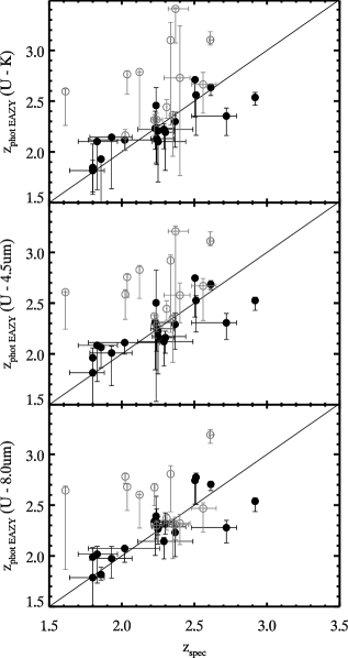
Figure 3.— Top panel: EAZY $z_{\mbox{\scriptsize phot}}$ calculated using the U$\rightarrow$K photometry vs. $z_{\mbox{\scriptsize spec}}$. Galaxies in the ECDFS, which has much poorer S/N JHK photometry than the MUSYC deep fields are plotted as open grey circles. Middle panel: Same as top panel but for $z_{\mbox{\scriptsize phot}}$’s determined with U$\rightarrow$4.5$\micron$ photometry. Bottom Panel: Same as top panel but for $z_{\mbox{\scriptsize phot}}$’s determined with U$\rightarrow$8.0$\micron$ photometry. The IRAC data does not improve the $z_{\mbox{\scriptsize phot}}$ of galaxies with good S/N JHK photometry. It does reduce the systematic overestimate of $z_{\mbox{\scriptsize phot}}$ for galaxies with poorer S/N JHK photometry, but only by 0.1 in $\delta$$z$, and only when all four IRAC channels are used. This shows that high S/N JHK photometry is significantly more valuable than IRAC data when determining the $z_{\mbox{\scriptsize phot}}$ of galaxies at $z\sim$ 2.3.

4.3. Reduction of Systematic Errors in Stellar Population Parameters with IRAC Data

Examination of the SEDs in $\S$ 4.1 showed that when the IRAC data were included in the fits to the U$\rightarrow$z^′+NIRspec data, the stellar population parameters of most galaxies remain consistent within the 1$\sigma$ uncertainties. Although consistent, the differences may be systematic, which could change the mean stellar population parameters of the sample. In this section we quantitatively check for systematic differences in the mean parameters with the inclusion of the IRAC data.
In Table 3 we list the mean value of the parameters determined with different subsets of the data compared to the mean value determined using the full U$\rightarrow$8$\micron$+NIRspec data set. Specifically, we compare parameters from fits to the broadband photometry and NIR spectroscopy without the IRAC data (U$\rightarrow$z^′+NIRspec, i.e., the same data as used in the fits by K08), broadband photometry including the IRAC data (U$\rightarrow$8$\micron$), and broadband photometry without IRAC data (U$\rightarrow$K). When fitting the broadband data we leave redshift as a free parameter in order to preserve systematic differences that may result from either random or systematic errors in $z_{\mbox{\scriptsize phot}}$. The uncertainties listed in Table 3 are standard errors of the mean ($\sigma$/$\sqrt{N}$). More details of the uncertainties and histograms that show the shape of the distributions are presented as an Appendix.
Table 3 shows that changes in the mean values of M${}_{\mbox{\scriptsize star}}$, $\tau$, $\langle t\rangle_{\mbox{\scriptsize SFR}}$, A_v, and SFR determined without the IRAC data (U$\rightarrow$z^′+NIRspec) compared to those determined with the IRAC data (U$\rightarrow$8$\micron$+NIRspec) are all consistent within the statistical accuracy achievable with our sample, approximately 10%. This demonstrates that not only are the parameters determined by K08 consistent with those determined with the IRAC data, but that none of the differences serve to change the mean parameters of the sample in a systematic way.
The mean values of most parameters determined using the broadband data are also consistent with those determined using the U$\rightarrow$8$\micron$+NIRspec data. The only exception is M${}_{\mbox{\scriptsize star}}$, which appears to be overestimated by a factor of $\sim$ 1.3 (0.11 dex) when only U$\rightarrow$K photometry is used in the fitting. This systematic overestimate was also seen by K08 when they compared the M${}_{\mbox{\scriptsize star}}$ from fits to the U$\rightarrow$K data to those from the U$\rightarrow$z^′+NIRspec data. Given that M${}_{\mbox{\scriptsize star}}$ determined with both the U$\rightarrow$8$\micron$+NIRspec and U$\rightarrow$z^′+NIRspec data are consistent, our fits support the K08 conclusions. As discussed in K08, the systematic effect on M${}_{\mbox{\scriptsize star}}$ can lead to an overestimate of the number of massive galaxies at high redshift, and hence an underestimate of the evolution of the stellar mass density.
Interestingly, it appears that the systematic overestimate of M${}_{\mbox{\scriptsize star}}$ is removed when the IRAC data is included in the SED fits to the broadband data. Elsner et al. (2008) also saw a systematic reduction in M${}_{\mbox{\scriptsize star}}$ when including IRAC data in SED fitting of broadband photometry of $z\sim$ 2 galaxies. Their M${}_{\mbox{\scriptsize star}}$ was systematically reduced by a factor of 1.6, which is similar to our factor of 1.3. Shapley et al. (2005) and Wuyts et al. (2007) made the same comparison; however, neither found that adding IRAC data caused a significant systematic change in the mean M${}_{\mbox{\scriptsize star}}$ of their sample. Shapley et et al. (2005) did suggest that the M${}_{\mbox{\scriptsize star}}$ of a subsample of their galaxies was systematically reduced when IRAC data was included in the fitting.
Why does including the IRAC data remove the systematic overestimate of M${}_{\mbox{\scriptsize star}}$ in our sample? In $\S$ 4.2 we showed that the $z_{\mbox{\scriptsize phot}}$ were systematically overestimated for galaxies in the ECDFS field, and that the IRAC data reduced this systematic by $\sim$ 0.1 in $\Delta$$z$/(1 + $z$). If we remove the ECDFS galaxies and compare the mean values of M${}_{\mbox{\scriptsize star}}$ from the U$\rightarrow$K photometry again, we find that the systematic overestimate of M${}_{\mbox{\scriptsize star}}$ is reduced to a factor of 1.08 $\pm$ 0.10. This suggests that it is primarily the systematic overestimate of the $z_{\mbox{\scriptsize phot}}$, caused by low S/N JHK photometry that is responsible for the overestimate of M${}_{\mbox{\scriptsize star}}$. Given that Wuyts et al. (2007) already had high S/N JHK photometry, this may explain why they saw no change in M${}_{\mbox{\scriptsize star}}$ when the IRAC data was included in the fitting. Both the Elsner et al. (2008) and Shapley et al. (2005) studies use the same redshifts for their fits with and without IRAC data, which suggests that their differences may be more data-specific, i.e., depend on the combination of broadband filters. Shapley et al. (2005) suggest it may be caused by contamination of their observed K_s-band fluxes from H$\alpha$ emission.
In summary, our comparison shows that when comparing stellar population parameters determined with various permutations of the data, the only parameter that suffers a systematic bias at the $>$ 10% level is M${}_{\mbox{\scriptsize star}}$ when determined using the U$\rightarrow$K photometry. This bias can be removed by including either NIR spectroscopy or IRAC data in the fitting because both improve the $z_{\mbox{\scriptsize phot}}$. None of the other parameters, $\tau$, $\langle t\rangle_{\mbox{\scriptsize SFR}}$, A_v, or SFR show evidence for systematic differences at $>$ 10% even without using IRAC data or NIR spectroscopy in the fitting.

4.4. Improvement of Uncertainties in Stellar Population Parameters with IRAC Data

Although the IRAC data do reduce the systematic errors in $z_{\mbox{\scriptsize phot}}$ and M${}_{\mbox{\scriptsize star}}$ for our sample, there are no changes in the mean values of the other stellar population parameters. This suggests that the IRAC data do not improve the accuracy for the majority of stellar population parameters. In this section we examine if including the IRAC photometry improves the uncertainties in the parameters determined for individual galaxies.
A simple test is to compare the parameter uncertainties computed using the Monte Carlo method. While potentially informative, such a comparison requires the uncertainties themselves to be robust, even in the case of sparse data. A direct way to test for an improvement is to measure the distribution of parameters computed without IRAC data relative to the distribution computed with IRAC data. The rms scatter of this distribution is a metric of the average uncertainty in a parameter for the sample, independent of the method used to estimate the uncertainties for individual galaxies.
Measuring a relative distribution of parameters requires a comparison sample. Since we do not have independent knowledge of the parameters without measurement uncertainty, we will assume that the parameters determined using the U$\rightarrow$8$\micron$+NIRspec data are likely to be the most precise, and compute the standard deviation ($\sigma$) of parameters determined without the IRAC data relative to these. A more detailed discussion of these comparisons, as well as histograms of the distributions are presented in the Appendix. In Figure 4 we graphically summarize the result of the comparisons for the parameters M${}_{\mbox{\scriptsize star}}$, $\tau$, $\langle t\rangle_{\mbox{\scriptsize SFR}}$, A_v, and SFR, computed using the U$\rightarrow$K, U$\rightarrow$8$\micron$, U$\rightarrow$z^′+NIRspec, and U$\rightarrow$8$\micron$+NIRspec data.
The left panel shows the $\sigma$ of the logarithm of the parameter distributions computed using each subset of the data plotted as a function of the $\sigma$ of the parameter distribution from the U$\rightarrow$8$\micron$+NIRspec data. In order to compare parameters with different units we use the fractional scatter in each parameter ($\sigma$/mean). Reading from left to right along the X-axis of Figure 4 shows which parameters are determined with the best precision using the U$\rightarrow$8$\micron$+NIRspec data.
The Y-axis of Figure 4 shows the logarithm of the scatter in parameters determined using the U$\rightarrow$K, U$\rightarrow$8$\micron$, and U$\rightarrow$z^′+NIRspec data which are plotted as green diamonds, blue squares, and red circles, respectively. The one-to-one relation is plotted as a dotted line. If a data point lies on that line it indicates that the precision of that parameter, with the given subset of data, is as good as the precision of that parameter attainable with the entire dataset.
Figure 4 shows some interesting trends, perhaps the most unsurprising of which is that the uncertainties in parameters determined using the U$\rightarrow$K data are always the largest. Adding either the NIR spectroscopy, the IRAC data, or the combination of the two significantly improves the uncertainties in all parameters. If we compare the uncertainties in parameters determined with the U$\rightarrow$8$\micron$ data (blue squares) to those determined with the U$\rightarrow$z^′+NIRspec (red circles) we can assess which parameters are most improved with each type of data, as well as the size of the improvement.
Examining the constraints from the U$\rightarrow$8$\micron$ data, it is clear that the IRAC data is most useful for constraining the M${}_{\mbox{\scriptsize star}}$, A_v, and SFR. Interestingly, adding the NIR spectroscopy in combination with the IRAC data does not further improve these parameter estimates. The U$\rightarrow$z^′+NIRspec data shows that the NIR spectroscopy is most useful for constraining the $\langle t\rangle_{\mbox{\scriptsize SFR}}$  and $\tau$ of the models; however, the uncertainty in both of these parameters can be further improved by including the IRAC data. The NIR spectroscopy also improves the M${}_{\mbox{\scriptsize star}}$ significantly, but including the IRAC data makes the constraints only $\sim$ 5% better.
Why do the different types of data affect the parameters in these ways? How can IRAC data improve SFR estimates, when it primarily traces the old stellar population? Although young-and-dusty and old-and-quiescent systems are difficult to distinguish with data that covers only the rest-frame UV to optical SED, they are separable once rest-frame NIR data is available (e.g., $\S$ 4.1, Labbé et al. 2005; Williams et al. 2008). This is not because the NIR wavelength range itself is particularly valuable, but because it completes the coverage of the part of a galaxy’s SED that is dominated by light from stellar photospheres. In turn this improves the constraints on the A_v, because A_v changes the broad shape of the stellar SED. In the $\tau$-models the SFR is not a quantity that is fit for, instead it is inferred from the number of $e$-folding times ($t$/$\tau$), scaled by the M${}_{\mbox{\scriptsize star}}$, and corrected for the A_v. Improved constraints on A_v lead to better SFRs, and hence IRAC data actually improves estimates of SFRs from SED fitting.
The NIR spectroscopy adds both a $z_{\mbox{\scriptsize spec}}$, as well as high-resolution information on the SED near the Balmer/4000Å break. As shown by K08, it is the high resolution information near the Balmer/4000Å  break that drives the improvement in both $t$ and $\tau$. Interestingly, the IRAC data still helps to improve the constraints on these parameters further. Most likely this is because it traces the old stellar population, which in tandem with the optical data constrains the ratio of old stars to young stars, and hence the number of $e$-folding times, which is directly related to both $t$ and $\tau$.
Perhaps the most remarkable result from Figure 4 is that for our sample, the parameters M${}_{\mbox{\scriptsize star}}$ and SFR are as well-determined from the U$\rightarrow$8$\micron$ photometry and $z_{\mbox{\scriptsize phot}}$, as they are from the U$\rightarrow$8$\micron$+NIRspec data and $z_{\mbox{\scriptsize spec}}$. This suggests that deep broadband photometry that extends into the rest-frame NIR can potentially provide unbiased high-quality estimates of the M${}_{\mbox{\scriptsize star}}$ and SFR for massive galaxies at 2 $<z<$ 3. NIR spectroscopy is extremely valuable for getting accurate rest-frame colors using $z_{\mbox{\scriptsize spec}}$ (e.g., K08), identifying AGN (e.g., Kriek et al. 2007), and to provide an independent check on SFRs from emission line fluxes (e.g., Erb et al. 2006); however, it does not significantly improve the constraints on M${}_{\mbox{\scriptsize star}}$ or SFR from the SED fits if IRAC data is available.

4.5. How Well Can We Constrain Stellar Populations Parameters with SEDs?

Given that our current sample of galaxies has the best-constrained SEDs of $z\sim$ 2.3 galaxies currently available, we can estimate the best-possible constraints on stellar population parameters that can be determined from SED fitting ignoring systematic effects such as choice of metallicity, IMF, and dust law. Assuming that the BC03 models with solar metallicity, a Salpeter IMF, and a Calzetti et al. (2000) dust law create an appropriate set of template SEDs, the X-axis of Figure 4 shows that the SED fitting best-constrains the parameters M${}_{\mbox{\scriptsize star}}$, A_v, and $\langle t\rangle_{\mbox{\scriptsize SFR}}$. Using the U$\rightarrow$8$\micron$+NIRspec data, M${}_{\mbox{\scriptsize star}}$ can be determined to $\pm$ 0.12 dex, $\langle t\rangle_{\mbox{\scriptsize SFR}}$  to $\pm$ 0.26 dex, and A_v to $\pm$ 0.3 mag. Interestingly, when only broadband U$\rightarrow$8$\micron$ data is used, the constraints on these parameters are similar, $\pm$ 0.11 dex, $\pm$ 0.36 dex, and $\pm$ 0.3 mag, for M${}_{\mbox{\scriptsize star}}$, $\langle t\rangle_{\mbox{\scriptsize SFR}}$, and A_v, respectively.
The $\tau$ and SFR, are not as well-determined as the other parameters. With the entire U$\rightarrow$8$\micron$+NIRspec data set the scatter in $\tau$ and SFR are factors of 2.5 and 2.8, respectively. The uncertainty in the SFR with the broadband data alone is still a factor of 2.8; however, the uncertainty in $\tau$ is much worse, a factor of 4.6. .
Overall, this exercise shows that the best constrained parameters of individual galaxies in our sample from SED fitting are M${}_{\mbox{\scriptsize star}}$, $\langle t\rangle_{\mbox{\scriptsize SFR}}$ , and A_v. As we will demonstrate in the $\S$ 5, these uncertainties are now small enough that they are comparable to the level of the systematic errors caused by the uncertainty in SPS code, metallicity, dust law and IMF.

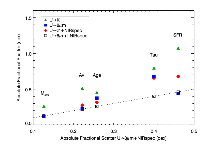
Figure 4.— The logarithm of the absolute fractional scatter in parameters, Log($\sigma$/mean), determined with various subsets of the data (U$\rightarrow$K, U$\rightarrow$8$\micron$, U$\rightarrow$z^′+NIRspec) plotted versus the logarithm of the absolute fractional scatter determined with the entire dataset (U$\rightarrow$8$\micron$+NIRspec). The dotted line has a slope of unity. Reading along the X-axis, the best constrained parameters are M${}_{\mbox{\scriptsize star}}$, A_v, and $\langle t\rangle_{\mbox{\scriptsize SFR}}$, which have rms scatters of $\sim$ 0.12 - 0.25 dex. The $\tau$ and SFR are not as well constrained from the SED alone, and have a scatter of a factor of $\sim$ 2-3.

5. Comparison of SPS Codes

In this section we fit the full U$\rightarrow$8$\micron$+NIRspec photometric dataset to a grid of $\tau$-models from the SPS codes of BC03, M05, and CB08. We examine the overall quality of the fits based on the $\chi_{r}^{2}$ statistic as well as the residuals from the mean SEDs to test whether a particular set of models provides a better description of the data. Given the different treatment of the TP-AGB phase of stellar evolution in the M05 and CB08 models compared to the BC03 models and the larger rest-frame NIR fluxes this produces, we compare fits with and without the IRAC data as a test of how well the models describe the SEDs in the rest-frame NIR. We also examine the systematic differences in the stellar population parameters determined with the different codes and their implications for studies of the stellar populations of distant galaxies. Throughout this comparison we assume solar metallicity, a Salpeter IMF, and the Calzetti et al. (2000) dust law as a “control” model.

5.1. Comparison of Models When Excluding IRAC

Our first comparison of the models is made using the U$\rightarrow$z^′+NIRspec data which effectively spans the UV through optical wavelength range for the galaxies in our sample. The parameters determined from these fits are listed in Table 1. In the top panels of Figure 5 we plot the $\chi_{r}^{2}$’s of the fits to the M05 and CB08 models against those from the fits to the BC03 models. Figure 5 shows that there is a large range of $\chi_{r}^{2}$ values for the fits; however, the majority of the systems, 26/34 (76%) are reasonably well described by the models, having $\chi_{r}^{2}$ $<$ 2. This shows that even with the high-resolution photometric data available from the NIR spectroscopy, simple $\tau$-models from all three SPS codes can still successfully reproduce the SEDs of the majority of $z\sim$ 2 galaxies.
Comparison of the $\chi_{r}^{2}$ values shows that the BC03 models have the lowest $\chi_{r}^{2}$ for 9/34 galaxies (26%), the M05 models have the lowest $\chi_{r}^{2}$ for 15/34 galaxies (44%), and the CB08 models have the lowest $\chi_{r}^{2}$ for 10/34 galaxies (29%). This demonstrates that within our sample there is no statistically significant evidence that one of the models provides the best fits more frequently than the others. Summing the $\chi_{r}^{2}$ values for all 34 galaxies results in total $\chi_{r}^{2}$’s of 57.72, 60.54, and 58.02 for the BC03, M05, and CB08 models, respectively. These imply an average $\chi_{r}^{2}$ of 1.70 $\pm$ 0.03, 1.78 $\pm$ 0.03, and 1.71 $\pm$ 0.03 for the BC03, M05, and CB08 models, respectively, where the quoted errors are standard errors of the mean. This suggests that the BC03 and CB08 models may provide modestly better fits on average to the rest-frame UV through optical SEDs than the M05 models; however, the majority of this difference is caused by a few galaxies that are fit much better by the BC03 and CB08 models (e.g., galaxy HDFS2-509 and 1256-1967)
It is worth noting that in Figure 5 the $\chi_{r}^{2}$ values of the BC03 and CB08 models are nearly identical for all galaxies, whereas there is a larger scatter in the $\chi_{r}^{2}$’s between the BC03 models and the M05 models. This confirms that the SEDs in the BC03 and CB08 models appear to be nearly identical in the rest-frame UV through optical wavelength range. In $\S$ 5.2 we will show that the fits to the rest-frame UV to NIR using the BC03 and CB08 models are quite different; and the current comparison makes it clear that those differences must be driven exclusively by the rest-frame NIR part of the SED.
Overall, based on the average $\chi_{r}^{2}$, the BC03 and CB08 models perform slightly better than the M05 models at fitting the rest-frame UV to optical SEDs, but the difference is small ($\sim$ 5% in $\chi_{r}^{2}$) and only significant at $\sim$ 1.5$\sigma$ within our sample of 34 galaxies.

Figure 5.— Top Panels: Comparison of $\chi_{r}^{2}$ values for fits without the IRAC data included using models from the M05 code vs. the BC03 code (left) and the CB08 code vs. the BC03 code (right). The $\langle\chi_{r}^{2}\rangle$ values are 1.70 $\pm$ 0.03, 1.78 $\pm$ 0.03, and 1.71 $\pm$ 0.03 for the BC03, M05, and CB08 models, respectively. This suggests that on average the BC03 and CB08 models may provide slightly better fits to the rest-frame UV to optical of young galaxies than the M05 models. Bottom Panels: Comparison of $\chi_{r}^{2}$ values for fits including the IRAC data using models from the M05 code vs. the BC03 code (left) and the CB08 code vs. the BC03 code (right). The $\langle\chi_{r}^{2}\rangle$ values are 1.79 $\pm$ 0.03, 1.77 $\pm$ 0.03, and 1.85 $\pm$ 0.03 for the BC03, M05, and CB08 models, respectively. Based on this comparison, all three codes perform equally well at fitting the rest-frame UV to NIR SEDs of young galaxies.

5.2. Comparison of Models When Including IRAC

We next compare how well the models describe the entire rest-frame UV to NIR SED of the galaxies by fitting the U$\rightarrow$8$\micron$+NIRspec data. The best fit SEDs from each SPS code are plotted in units of F_ν vs. $\lambda$ in Figures 6 and 7. The black line, green line, and blue line are the best fits using the BC03, M05, and CB08 models, respectively. The best fit stellar population parameters, their uncertainties, and the $\chi_{r}^{2}$ of the best fits are listed in Table 1. We plot the $\chi_{r}^{2}$’s of the fits to the M05 and CB08 models against those from the fits to the BC03 models in the bottom panels of Figure 5.
Comparison of the $\langle\chi_{r}^{2}\rangle$’s in the top and bottom panels Figure 5 shows that the variance in $\chi_{r}^{2}$’s between models is significantly larger when the rest-frame NIR is included in the fitting; however, the frequency with which each model provides the best fit is still similar. The BC03 models have the lowest $\chi_{r}^{2}$ for 11/34 (32%) of the galaxies, the M05 models have the lowest $\chi_{r}^{2}$ for 12/34 (35%) of the galaxies, and the CB08 models have the lowest $\chi_{r}^{2}$ for 11/34 (32%) of the galaxies.
Totaling the $\chi_{r}^{2}$ for all fits with each SPS codes gives values of 62.80, 62.11, and 64.72 for the BC03, M05, and CB08 models, respectively. Converting the total $\chi_{r}^{2}$’s to a $\langle\chi_{r}^{2}\rangle$ per galaxy for our sample gives values of 1.85 $\pm$ 0.03, 1.83 $\pm$ 0.03, and 1.90 $\pm$ 0.03 for the BC03, M05, and CB08 models, respectively, where the errors are the standard error of the mean. Interestingly, when the rest-frame NIR is included, the M05 models describe the SEDs slightly better than both the BC03 and CB08 models on average. The difference is not significant when comparing the BC03 and M05 models; however, it is significant at $\sim$ 1.5$\sigma$ when comparing the M05 and CB08 models. Maraston et al. (2006) found similar results using a sample of 7 galaxies at 1.4 $<z<$ 2.7 selected from the GOODS survey. For their sample the $\langle\chi_{r}^{2}\rangle$ was 1.38 $\pm$ 0.10 for fits with the M05 models, and 1.51 $\pm$ 0.10 for fits with the BC03 models, where we have computed the error bars based on the standard error of the mean. Their results also show a small, but not statistically significant, advantage for the M05 models compared to the BC03 models when the entire rest-frame UV to NIR SED is fit.
If the M05 models had the largest $\langle\chi_{r}^{2}\rangle$ when fitting the rest-frame UV to optical SEDs of the galaxies, but the smallest $\langle\chi_{r}^{2}\rangle$ when the rest-frame NIR data is included, it suggests that they may describe the rest-frame NIR for these galaxies better than both the BC03 and CB08 models. We test this by plotting the $\chi_{r}^{2}$ values obtained when fitting using only the U$\rightarrow$z^′+NIRspec data versus those obtained when fitting the U$\rightarrow$z^′+NIRspec+IRAC data for all three SPS codes in Figure 8. Galaxies that have much poorer fits when the rest-frame NIR is included will lie to the right of the dotted line in Figure 8.
Before we discuss the $\chi_{r}^{2}$ values from fits with and without the rest-frame NIR data, it is worth noting that the fraction of massive galaxies that host an AGN at $z\sim$ 2 is much higher than at lower redshift (e.g. Kriek et al. 2007, Daddi et al. 2007). The presence of a dusty AGN can cause significant emission at rest-frame NIR wavelengths (e.g., Donley et al. 2008, and references therein), and therefore can “contaminate” the stellar SED in the rest-frame NIR. Such systems are now being identified at high redshift using the presence of excess emission at $\lambda$ $>$ 1.6$\micron$, rest-frame. Galaxies with a dusty AGN are frequently referred to as power-law galaxies (PLGs) because the strong NIR emission at $\lambda$ $>$ 1.6$\micron$ from the AGN overpowers the stellar emission removing the turnover in the SED at 1.6$\micron$ from the peak of the stellar emission, and making the SED appear more like a power-law. Given that the SPS models do not include an AGN component, we expect any galaxies identified as PLGs will be fit much more poorly when the rest-frame NIR is included. Poor fits to these galaxies in the rest-frame NIR probably does not reflect a deficiency with the models and therefore we need to identify any PLGs within our sample.
We identified PLGs by fitting the IRAC data for each galaxy to a power-law of the form $f_{\nu}\propto\nu^{\alpha}$. Galaxies fit with $\alpha$ $>$ -0.5 are considered PLGs, and therefore likely candidates for hosting a dusty AGN (e.g., Alonso Herrero et al. 2006, Donley et al. 2007). The properties of these galaxies and their overlap with emission-line AGN (Kriek et al. 2007) will be presented in more detail, and including MIPS 24$\micron$ observations, in a future paper. Here we only discuss them as they are relevant to SED fitting in the rest-frame NIR.
The PLGs are plotted as open red circles in Figure 8. Interestingly, not only do most of the PLGs have significantly poorer fits in the rest-frame NIR than the average galaxy, they also have significantly poorer fits in the rest-frame UV to optical than the average galaxy. This suggests that if these systems do have a dusty AGN, the AGN may also emit radiation blueward of rest-frame 1.6$\micron$ and “contaminate” this part of the SED as well.
Excluding the PLGs, we can see that for the M05 models, very few galaxies have significantly higher $\chi_{r}^{2}$ values when the rest-frame NIR data are included in the fit. For the BC03 and CB08 models, there are some non-PLG systems where the fits are much worse when the rest-frame NIR data is included; however, there are only a handful of such galaxies. The most discrepant galaxies in the BC03 models are 1030-1531, 1256-519, and 1256-1967. Galaxy 1256-519 has a poor fit with the IRAC data in all models; however, it is notable that 1030-1531 and 1256-1967 have $more$ flux in the rest-frame NIR than predicted by the BC03 models and are better described by the M05 and CB08 models. Interestingly, these two galaxies also have similar ages (0.47${}^{+0.09}_{-0.07}$, and 0.45${}^{+0.07}_{-0.16}$ Gyr) from the M05 fits, and are right in the middle of the age range were emission from TP-AGB stars is near the maximum for a range of metallicities (e.g. M05) suggesting that the different treatment of these stars in the M05 and CB08 models is the cause of the improved fit. Still, it is possible that these two galaxies could be modeled using a composite of young and old bursts with the BC03 code (e.g., Yan et al. 2004), and with only two non-PLG galaxies in the sample that would require such modeling to explain the SED, we suggest that there is only mild evidence at best from the $\chi_{r}^{2}$’s that the SEDs from the BC03 code require significant changes in the rest-frame NIR in order to match the observed SEDs of our galaxies.
This can also be seen in Figure 9 where we plot the residuals from the SEDs fit using models from the three SPS codes, corrected to the rest-frame. The solid line represents a running average of the 30 nearest points. The running average suggests that the BC03 models may underpredict the mean flux of the average galaxy in the wavelength range 1.0 - 1.8$\micron$; however, the difference is at most, 5-10%, conceivably within the allowable range of the uncertanties in the IRAC photometry. The residuals from the M05 and CB08 models do not show the same trend, suggesting that they may describe the rest-frame NIR SEDs of these galaxies slightly better than the BC03 models.
In summary, these comparisons show a few key results. Most importantly, based on the frequency of lowest $\chi_{r}^{2}$ and the $\langle\chi_{r}^{2}\rangle$ for all galaxies, we conclude that there is no significant evidence that any of the three SPS codes we tested describe the complete rest-frame UV to NIR SEDs of massive $z\sim$ 2.3 galaxies significantly better than the others. Comparison of the $\langle\chi_{r}^{2}\rangle$’s from fits with and without the rest-frame NIR data suggest that the BC03 and CB08 models may describe the rest-frame UV to optical SEDs of the galaxies slightly better than the M05 models, but that the latter may fit the rest-frame NIR better than the former. Still, the differences in the $\langle\chi_{r}^{2}\rangle$ between the models are always $<$ 5% and are only significant by $\sim$ 1.5$\sigma$ at most. The residuals from the fits also seem to show that the M05 and CB08 models describe the rest-frame NIR slightly better than the BC03 models, but again, the difference is at most 5-10%, and within the photometric errors. These comparisons suggest that it will be extremely difficult to refine the models based on the observed SEDs of young stellar populations at high redshift. Mostly likely such constraints will have to come from other avenues such as NIR spectroscopy of young stellar populations in the local universe (e.g., Riffel et al. 2008) or improved theoretical understanding of post main sequence stellar evolution (e.g., Marigo et al. 2008), or both.

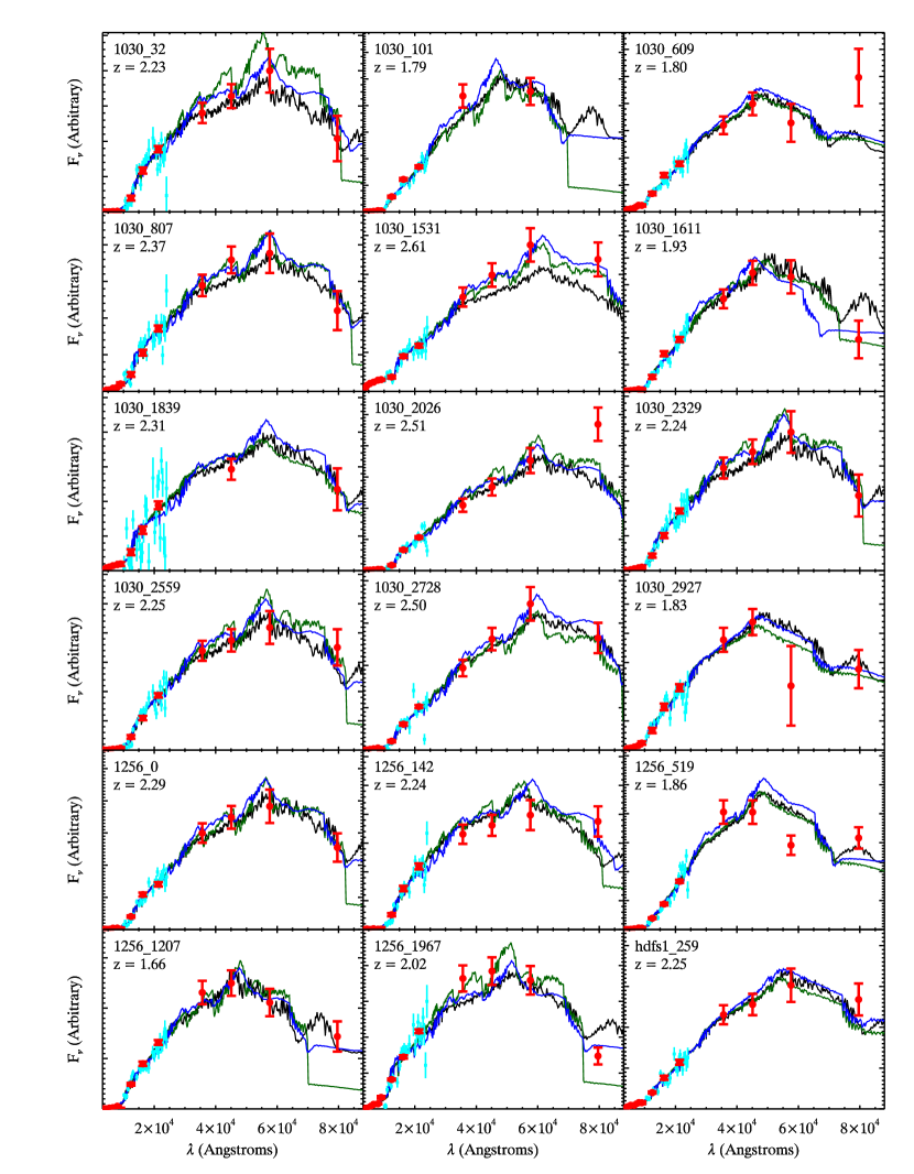
Figure 6.— SEDs fit with BC03 models (black), M05 models (green) and CB08 models (blue), plotted as F_ν vs. Log($\lambda$). Red points are the broadband photometric data and cyan points are the binned NIR spectroscopy.

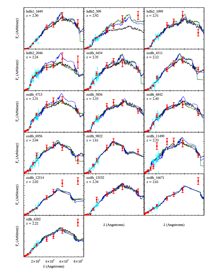
Figure 7.— As Figure 6.

5.3. How do best-fit parameters vary between SPS codes?

Although the three codes describe the overall shape of the SEDs of the galaxies equally well, the parameters of the best fit SEDs from the codes imply significantly different stellar populations for the same galaxies. In Figure 10 we plot the SED parameters determined from the U$\rightarrow$8$\micron$+NIRspec data using the M05 and CB08 models against those determined using the BC03 models as solid circles and open diamonds, respectively.

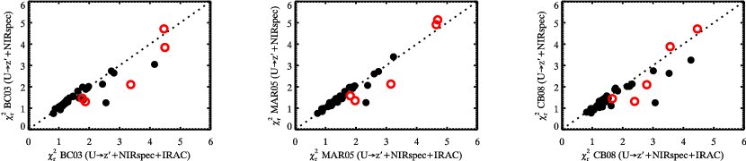
Figure 8.— Left Panel: Comparison of $\chi_{r}^{2}$ values for fits with and without the IRAC data using the BC03 models. Middle Panel: Same as left panel but for fits with the M05 models. Right Panel: Same as left panel but for fits with the CB08 models. Open red circles represent galaxies whose SEDs follow a power law in the IRAC bands of the form f_ν $\propto$ $\nu^{\alpha}$, where $\alpha$ $<$ -0.5. These galaxies are commonly defined as “power-law galaxies” and likely have the rest-frame NIR dominated by emission from dust heated by an AGN. The M05 models show the least increase in $\chi_{r}^{2}$ when the rest-frame NIR data is included in the fitting; however, the BC03 and CB08 models have only a few non-power-law galaxies that have notably worse fits when the rest-frame NIR data is used in the fitting.

5.3.1 Differences in Stellar Populations Between M05 and BC03 Models

The mean and median ratio of stellar population parameters determined with the M05 and BC03 models are listed in Table 4. The most significant difference between these models is in the median M${}_{\mbox{\scriptsize star}}$. From Figure 10 we can see that the median M${}_{\mbox{\scriptsize star}}$ from the M05 models is 0.63 that of the BC03 models, and appears to be a systematic offset, independent of the mass of the galaxy. If we divide the galaxies into two samples, those with detected emission lines in the NIR spectrum (hereafter EL-galaxies) and those without detectable emission lines (hereafter NEL-galaxies) the systematic change in M${}_{\mbox{\scriptsize star}}$ for both of these groups is 0.63 and 0.69, respectively, nearly identical to the median difference of 0.63 for the whole sample. This offset in M${}_{\mbox{\scriptsize star}}$ is similar to those measured by Maraston et al. (2006) and Wuyts et al. (2007) who saw ratios of 0.58 and 0.72, respectively.
Comparing the best fit values of $\tau$ between the models shows that the M05 models prefer slightly lower values, they have a median $\tau$ that is 0.75 that of the BC03 $\tau$. This difference is driven mostly by the EL-galaxies which have a $\tau$ of 0.66 times the BC03 value; whereas the NEL-galaxies have a $\tau$ 0.83 times the BC03 value. This suggests that in the M05 models, the SFH of EL-galaxies is burstier than for the BC03 models; however, we note that $\tau$ is one of the poorest constrained parameters when fitting the SEDs alone.
If we compare the $\langle t\rangle_{\mbox{\scriptsize SFR}}$  of the M05 models to the BC03 models we find that they are lower by a factor of 0.65. Again, this ratio is similar to the ratios of 0.58 and 0.51 found by Maraston et al. (2006) and Wuyts et al. (2007), respectively. However, unlike M${}_{\mbox{\scriptsize star}}$, the age differences are particularly pronounced between the EL- and NEL-galaxies. The ratio of ages of the NEL-galaxies between the M05 models and BC03 models is 1.03, but for the EL-galaxies the ratio is 0.42. The age of the stellar population is closely tied to the SFH, as the shape of the SED is primarily determined by the number of e-folding times of the SFH, which is effectively the ratio of $t$/$\tau$. Given that there are differences in $\tau$ between the models, a similar trend in $t$ and $\langle t\rangle_{\mbox{\scriptsize SFR}}$  is expected in order to preserve the number of e-folding times.
Due to these differences in $\tau$ and $\langle t\rangle_{\mbox{\scriptsize SFR}}$  we also expect a significant difference in the SFRs for EL- and NEL-galaxies. The median ratio of SFRs is 1.12; however, it is 1.58 and 0.33 for EL- and NEL-galaxies, respectively (the clear trend can also be seen in Figure 11). In the M05 models NEL-galaxies have significantly less SF than the BC03 models would predict, whereas EL-galaxies are more active than the BC03 models would predict, leading to a more bimodal galaxy distribution, if galaxies are classified by SFR.
The final parameter we consider is the A_v of the galaxies. The median $\Delta$A_v for the sample (where $\Delta$A_v $\equiv$ A_v,M05-A_v,BC03) is 0.0; however, $\Delta$A_v = 0.1 for the EL-galaxies, and $\Delta$A_v = -0.4 for the NEL-galaxies. The M05 models require far less dust to fit the NEL-galaxies’ SEDs, and to first order this explains why the NEL-galaxies have smaller M${}_{\mbox{\scriptsize star}}$ when fit with the M05 models, despite the fact that they have similar $\tau$ and $\langle t\rangle_{\mbox{\scriptsize SFR}}$ . Maraston et al. (2006) also showed that when fitting without dust the M05 models produce fits with significantly lower $\chi_{r}^{2}$ than the BC03 models, suggesting they require less dust to reproduce the SEDs of their sample as well.
In summary, galaxies fit with the M05 models have a median values of 0.63$\cdot$M${}_{\mbox{\scriptsize star}}$, 0.65$\cdot$$\langle t\rangle_{\mbox{\scriptsize SFR}}$ , and 0.75$\cdot$$\tau$ with similar A_vs and SFRs when compared to galaxies fit with the BC03 models, consistent with earlier studies. However, breaking the sample up into EL- and NEL-galaxies shows more interesting trends. In the M05 models EL-galaxies have shorter timescales for SF and younger ages and this leads to SFRs that are higher by a factor of 1.58. Conversely, for NEL-galaxies the values of $\tau$ and $\langle t\rangle_{\mbox{\scriptsize SFR}}$  are fairly similar between the M05 models and the BC03 models; however the A_v is 0.4 mag less in the M05 models, and the SFRs are only 0.33 of the BC03 value. Overall, the M05 models produce a more strongly bi-modal population of galaxies at $z\sim$ 2.3. EL-galaxies have a shorter-timescale for SF, and larger SFRs; whereas NEL-galaxies have less dust and are more quiescent.

Figure 9.— Residuals from the SED fits using the BC03, M05, and CB08 models corrected to the rest-frame. The residuals are the fractional residual where $\Delta f_{\lambda}/f_{\lambda}\equiv f_{obs}-f_{model}/f_{obs}$. The black line represents a running average of the nearest 30 data points. The running average suggests that the M05 and CB08 models may describe the SEDs of the galaxies better in the range 1.0 x 10⁴ Å $<\lambda<$ 1.8 x 10⁴ Å; however, the improvement is $\sim$ 5-10%, well within the photometric errors.

5.3.2 Differences in Stellar Populations from the CB08 Models

Parameters determined from the CB08 models also have marked differences from those determined with the BC03 models. Similar to the M05 models, M${}_{\mbox{\scriptsize star}}$ from the CB08 models is lower by a factor of 0.74. Dividing these into the EL- and NEL-galaxy categories we find that for the EL-galaxies M_star,CB08/M_star,BC03 = 0.77 and NEL-galaxies M_star,CB08/M_star,BC03 = 0.70. This demonstrates that similar to the M05 fits, the differences in M${}_{\mbox{\scriptsize star}}$ are not a strong function of SED type and are a systematic offset between the models. Of interest, this difference in M${}_{\mbox{\scriptsize star}}$ is less dramatic than the factor of 0.32 found by Bruzual (2007) when fitting the galaxies used in Maraston et al. (2006); however, they compared M${}_{\mbox{\scriptsize star}}$ using fits without including dust extinction. Clearly, once dust is included in the fitting the differences in M${}_{\mbox{\scriptsize star}}$ are not as significant.
The median $\tau$ is similar between the CB08 and BC03 fits; however, like the M05 fits, its dependence is strongly bimodal. In the CB08 fits, the EL-galaxies have $\tau$’s which are 0.66 that of the BC03 $\tau$’s. This behavior is similar to the M05 EL-galaxies, which also have shorter SF timescales. The NEL-galaxies actually have larger $\tau$’s in the CB08 models compared to the BC03 models by a factor of 1.25.
Unlike the M05 models, the $\langle t\rangle_{\mbox{\scriptsize SFR}}$ of galaxies in the CB08 models are actually older than the BC03 models, with a median value 1.24 times larger. This dependence is again strongly bimodal, with the EL-galaxies having a $\langle t\rangle_{\mbox{\scriptsize SFR}}$ 0.96 times the BC03 models, but the NEL-galaxies are older, with $\langle t\rangle_{\mbox{\scriptsize SFR}}$_,CB08 = 1.46$\langle t\rangle_{\mbox{\scriptsize SFR}}$_,BC03. Interestingly, this gives the same relative behavior as the M05 models, i.e., the EL-galaxies get younger relative to the NEL-galaxies; however, with the CB08 models it is the NEL-galaxies that get older while the EL-galaxies stay the same age. In the M05 models, the EL-galaxies get younger, but the NEL-galaxies stay the same age.
The median extinction is lower in the CB08 models compared to the BC03 models, being $\Delta$A_v = -0.4 for all galaxies. The effect is stronger for NEL-galaxies, which have $\Delta$A_v = -0.6, compared to the EL-galaxies which have $\Delta$A_v = -0.2.
Overall, the net effect of using the CB08 models compared to the BC03 models is that the mean M${}_{\mbox{\scriptsize star}}$ of galaxies is lower by a factor of 0.74, and perhaps more importantly, the galaxy population becomes more bimodal in several parameters. This is similar to the result from the M05 models; however, the bimodalism is driven by movement in different types of galaxies. In the CB08 models compared to the BC03 models EL-galaxies have lower $\tau$’s, but similar $\langle t\rangle_{\mbox{\scriptsize SFR}}$ ’s, giving them a slightly burstier SFH. This is different than the M05 models which are both significantly younger and have even smaller $\tau$’s. In the CB08 models the NEL-galaxies have both longer $\tau$’s, older ages, and surprisingly, less dust. In the M05 models, the NEL-galaxies had similar $\tau$’s, and $\langle t\rangle_{\mbox{\scriptsize SFR}}$  as the BC03 models.
If we divide the galaxy population by SFR in both the M05 and CB08 model it is more bimodal than in the BC03 models. For the M05 models, the change is dominated by the EL-galaxies, which are notably younger and bustier with higher SFRs than their BC03 counterparts. For the CB08 models, the bimodality is driven by the NEL-galaxies which become older, with longer $\tau$ and smaller SFRs than their BC03 counterparts.

Figure 10.— Ratio of best-fit CB08 (open triangles) and M05 (filled circles) SED parameters to the best fit BC03 SED parameters as a function of the BC03 parameters. The median M05 fit is 0.63 of M${}_{\mbox{\scriptsize star}}$, and 0.65 of $\langle t\rangle_{\mbox{\scriptsize SFR}}$ compared to the BC03 fits, while the $z$, SFR, and A_v are similar. The median CB08 fit is 0.74 of M${}_{\mbox{\scriptsize star}}$, and 1.24 of $\langle t\rangle_{\mbox{\scriptsize SFR}}$, and has 0.4 mag less A_v compared to the BC03 fits, while the $z$, SFR are similar

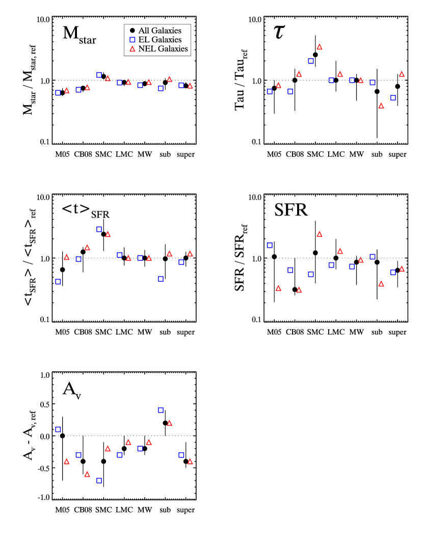
Figure 11.— Difference in the median value of parameters fit using the various SPS codes, dust laws, and metallicities (see text) compared to the “control” model. Open blue squares represent galaxies with detectable emission lines and open red triangles represent galaxies without detectable emission lines. The filled black circles are the median for all galaxies. The lines denote the range that contains 50% of the galaxies. Most of the largest systematic offsets are from the SPS codes, and their most significant effect is on M${}_{\mbox{\scriptsize star}}$, and $\langle t\rangle_{\mbox{\scriptsize SFR}}$, the two parameters best determined by the SED fitting.

6. Systematic Effects on Stellar Population Parameters from Metallicity and Dust Law

As we have shown in the previous section, SED fits using the current generation of SPS codes provide stellar populations parameters that suffer from significant systematic effects. In this section we quantify how large these systematic effects are relative to other known systematics such as the choice of dust law and metallicity.
We allow three dust laws to redden the SEDS: the Milky Way (MW) and Large Magellanic Cloud (LMC) dust laws determined by Fitzpatrick et al. (1986), and the Small Magellanic Cloud (SMC) dust law determined by Prévot et al. (1984). We also incorporate two new metallicities into the fits, a subsolar (Z = 0.2 Z_⊙), and supersolar (Z = 2.5 Z_⊙) population. For the BC03 models these are the m42, and m72 stellar populations, respectively.
In an attempt to isolate variables we use the BC03 models as our control SPS code. When comparing dust laws we assume solar metallicity as our control metallicity, and when comparing metallicities we assume a Calzetti et al. (2000) dust law as the control dust law. It is possible that using a different control model will affect some of these comparisons; however, the large number of potential permutations allowed in choosing the control model (there are 36 possible combinations of SPS code, dust law, and metallicity) require us to chose only one in order to make the interpretation of systematic effects tractable. Moreover, the most commonly used models for determining stellar population parameters thus far have been the BC03 models with solar metallicity and the Calzetti dust law, so systematic changes in parameters relative to this model are probably the most interesting for understanding the implications of assumptions made in previous work.
We first examine the effect of using the various dust laws on the parameter estimates. The ratios of parameters determined from fits using the SMC, MW, and LMC dust laws compared to those from the BC03_m62+Calzetti control model are listed in Table 5 and are plotted in Figure 11. The open red triangles and open blue squares represent the medians of the NEL-galaxies and EL-galaxies, respectively, and the black points denote the medians of the whole sample. The error bars on the black points denote the range spanned by 50% of the sample. Figure 11 shows that when parameters determined using the LMC and MW dust laws are compared to those determined using the Calzetti law, the only parameter that is significantly different is the A_v. Parameters such as M${}_{\mbox{\scriptsize star}}$, $\tau$, $\langle t\rangle_{\mbox{\scriptsize SFR}}$ , and SFR only change systematically by of order $\sim$ 10%, and therefore appear to be robust regardless of whether the MW, LMC, or Calzetti dust laws are used. Furthermore, the changes do not appear to depend on the EL- and NEL-galaxy classification. As pointed out by Förster Schreiber et al. (2004), the lack of significant changes in parameters between these three dust laws is not surprising because they are fairly similar in shape. The only notable difference is that the Calzetti law lacks the 2175Å absorption feature and that the ratio of total to selective absorption is slightly higher, R_v = 4.05, compared to R_v = 3.1 for the MW and LMC laws.
Using the SMC dust law does cause some significant changes to several parameters. The median $\tau$ and $\langle t\rangle_{\mbox{\scriptsize SFR}}$  are larger by a factors of 2.5, and 2.8, respectively, and the median A_v is lower by 0.4 mag. The median SFR is similar; however, this results from a coincidental cancellation caused by the NEL-galaxies having SFRs a factor of $\sim$ 2 higher, and EL-galaxies having SFRs a factor of $\sim$ 2 lower. The SMC dust law has by far the strongest attenuation of all four dust laws at $\lambda$ $<$ is 2000Å rest-frame and therefore it requires stellar populations with more rest-frame UV flux to describe the SEDs. This leads to a preference for longer timescales for SF and older ages so that there is a contribution from both a young and old population simultaneously. Because of the shape of the SMC dust law, the fits prefer intrinsically redder stellar populations (i.e., those with older ages and longer $\tau$) and less dust, rather than short bursts with more dust. The preference for older ages and less dust would probably diminish if we used the SMC law with a subsolar metallicity population, which is intrinsically bluer and would allow for more dust and shorter timescales for SF.
Next we examine the effect on the parameters caused by varying the metallicity while holding the SPS model and dust law fixed. The median values of the parameters determined from those fits compared to the control models fits are listed in Table 6 and are also plotted in Figure 11. The choice of metallicity affects more parameters than does the choice of dust law; however, it is still a modest effect. The $\tau$ of the stellar populations is lower for both metallicities; however, the dependence for EL- and NEL-galaxies is reversed. The A_v depends on metallicity in the predictable way, with subsolar metallicity requiring more dust, and supersolar requiring less.
Perhaps what is most interesting about the variations in parameters caused by choice of dust law and metallicity is that other than the SMC dust law, their net systematic effect on M${}_{\mbox{\scriptsize star}}$, and $\langle t\rangle_{\mbox{\scriptsize SFR}}$ , the two parameters that are the best-determined using SED fitting ($\S$ 4.5) is fairly small, $\sim$ 10-20%. They do have larger effects on $\tau$ and SFR; however, these are the parameters that are most poorly determined using the SED fitting.
One disconcerting aspect of Figure 11 is that it shows clearly that it is the SPS codes that have the largest systematic effects on most parameters, and most importantly, that the largest systematic changes occur on the parameters that are best determined by the SED fitting: M${}_{\mbox{\scriptsize star}}$, $\langle t\rangle_{\mbox{\scriptsize SFR}}$ , and A${v}$. So, despite the fact that using the best data currently available we can constrain the M${}_{\mbox{\scriptsize star}}$, $\langle t\rangle_{\mbox{\scriptsize SFR}}$ , and A_v of individual galaxies to $\sim$ 0.1 dex, 0.3 dex, and $\pm$ 0.3 mag, respectively ($\S$ 4.5), it appears that systematic errors in these parameters from the various SPS codes dominate over random errors for all three parameters as they cause systematic uncertainties of roughly $\pm$ 0.3 dex in M${}_{\mbox{\scriptsize star}}$ and $\langle t\rangle_{\mbox{\scriptsize SFR}}$ , and $\pm$ 0.4 mag in A_v. This suggests than unless these systematic discrepancies between the SPS models are resolved, more multiwavelength data on the stellar component of the galaxy SED will not provide better constraints on the evolution of the stellar mass density in the universe, or the peak epoch of the formation of stars in the universe. Longer wavelength data that probes emission from dust (e.g., MIPS, ALMA) will almost certainly improve the SFR estimates; however, parameters determined from the stellar SED are now limited by systematic errors. Adding to the challenge is the analysis in $\S$ 5.2 that shows that even with the best constrained SEDs of young stellar populations currently available we will not be able to “fit out” these systematic problems, as all three models describe the SEDs equally well.

7. Implications: Confirmation of the Existence of a Substantial Population of Quiescent Galaxies at $z\sim$ 2.3

Using this sample of galaxies Kriek et al. (2006) have argued that $\sim$ 50% of K-selected galaxies at $z\sim$ 2.3 have strongly suppressed star formation based on their lack of observed emission lines and the fact that the rest-frame UV through optical SED was best described by an old quiescent population. Although they had the high-resolution NIR spectroscopy with which to model the stellar populations, Kriek et al. lacked the rest-frame NIR data from IRAC, without which it can be challenging to distinguish between young-and-dusty and old-and-quiescent populations (e.g., Labbé et al. 2005; Papovich et al. 2006; Wuyts et al. 2007, $\S$ 4). Although unlikely, they could not completely rule out the possibility that some fraction of the systems without emission lines could be highly extincted star forming galaxies rather than old and quiescent galaxies, and that the lack of emission lines and red optical colors are the result of significant dust obscuration. Here we examine the stellar populations from the SED fits of the EL and NEL galaxies to verify that the SEDs of the galaxies without emission lines are still consistent with them being systems with strongly suppressed star formation.
In the top panels Figure 12 we plot the specific star formation rate (SSFR), defined as SFR/M${}_{\mbox{\scriptsize star}}$, as a function of M${}_{\mbox{\scriptsize star}}$ for the EL galaxies (blue) and NEL galaxies (red). Candidate AGNs selected using the emission-line diagnostics in Kriek et al. (2007) as well as PLGs ($\S$ 5.2) are indicated with an open diamond. As we showed in $\S$ 6, the SPS codes have the largest systematic effects on M${}_{\mbox{\scriptsize star}}$ and SFR, and therefore we plot three versions of the diagram in Figure 12, one each for values determined using the three SPS codes.
It is clear from Figure 12 that the majority of galaxies without emission lines are found at the lowest SSFRs, whereas those with emission lines are found at the highest SSFRs. There are some notable model-dependent differences, with the M05 and CB08 models implying that the population of galaxies at $z\sim$ 2.3 has a more bimodal distribution of SSFRs, whereas the BC03 models suggest more of a continuum in SSFRs. This is apparent in the bottom panels of Figure 12, where we plot histograms of the SSFRs.
If we adopt the Kriek et al. (2008b) definition of quiescent systems as those that have SSFRs $<$ 0.05 Gyr^-1 (i.e., those that will increase their M${}_{\mbox{\scriptsize star}}$ by $<$ 5% in the next Gyr if the SFR remains at the same value), then we find that 13, 17, and 22 of the 34 galaxies (38%$\pm$12%, 50%$\pm$15%, 65%$\pm$18%) would be classified as quiescent based on the SED parameters from the BC03, M05, and CB08 models, respectively. These numbers are in good agreement with the 45${}^{+18}_{-12}$% determined by Kriek et al. (2006) based on the fraction of galaxies without emission lines and SED fitting. Despite the good agreement, there are a few subtle issues in the emission line classification. There are 16 galaxies without emission lines, and of these, 10, 12, and 15 of these would be considered quiescent based on their SED parameters from fits to the BC03, M05, and CB08 models, respectively. Therefore, the majority of systems without emission lines are quiescent; however, there is a non-negligible population ($\sim$ 6% - 33%) of galaxies without emission lines that do have some ongoing obscured star formation ranging from $\sim$ 10-850 M_⊙ yr^-1. Coincidentally, these few galaxies are canceled out in the overall quiescent fraction by a small fraction of emission line galaxies that are likely to be quiescent based on their SED, but probably have an AGN component that is responsible for the emission lines.
Taken together, these results suggest that the classification of $z\sim$ 2 galaxies into star forming and quiescent categories based on the presence/lack of emission lines and without any information on their SED is probably correct for the majority of systems ($\sim$ 70-90%); however, there is some cross contamination between the two categories from dusty star forming galaxies without emission lines, and quiescent galaxies with an emission line AGN. Within our sample these two populations appear to be small, and equally abundant and therefore cancel each other when estimating the quiescent fraction. As a result, the fraction of quiescent galaxies is roughly the same using the SED fits or the emission line classification. Our sample is fairly small, so it is not clear if the same cancellation would occur for larger samples.
Although the contamination in the emission line classification suggests we should appeal to the SED fits for a more robust classification, that method is not completely “clean” either: the quiescent fraction ranges by roughly a factor of 2 depending on which SPS code is used to model the SEDs. Considering this systematic effect and using the 1$\sigma$ confidence intervals from the models, we can conclude that the fraction of K-selected galaxies at $z\sim$ 2.3 that are classified as quiescent based on their SEDs ranges from as low as 26% to as high as 83% at 68% confidence, in good agreement with the value determined from the emission line fraction by Kriek et al. (2006). Clearly this uncertainty is large; however, even within our modest sample of 34 galaxies, the statistical uncertainties are already smaller than the systematic uncertainty from the SPS codes.
The histograms in Figure 12 suggest a more bimodal distribution of SSFRs when using the M05 and CB08 models compared to the BC03 models. Kriek et al. 2008b have shown that there is already a developed red sequence in the (U-B)_rest vs. M${}_{\mbox{\scriptsize star}}$ plane for this sample of galaxies and that most of the galaxies on the red sequence have low SSFRs as inferred from SED fits using the BC03 models. It is enticing to prefer SPS models that show the same bimodality in SSFRs as in rest-frame color; however, given that the current sample is small, and the random uncertainties in the SSFRs are large (factor of 2-3) it is better to defer such a comparison to a larger sample of galaxies (e.g., van Dokkum et al. 2009). It will be interesting to see how the SSFRs of galaxies in the larger sample relate to their rest-frame colors, which will be a much more accurately determined quantity using those data.

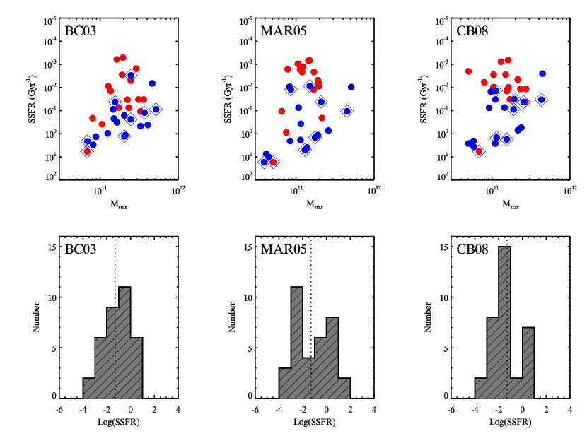
Figure 12.— Top Panels: Specific star formation rate (SSFR $\equiv$ SFR/M${}_{\mbox{\scriptsize star}}$) as a function of M${}_{\mbox{\scriptsize star}}$ determined from fits to the BC03, M05, and CB08 models. Galaxies with detected emission lines are plotted in blue, those without detectable emission lines are plotted in red. Candidate AGN (see text) are indicated using open diamonds. The three SPS models produce significantly different distributions in this parameter space; however, galaxies without emission lines typically have much lower SSFRs than those with emission lines. Bottom Panels: Histograms of the SSFR determined using models from the three SPS codes. The dashed line represents our definition of a quiescent galaxy (SSFR $<$ 0.05 Gyr^-1). Based on this definition, 38%$\pm$12%, 50%$\pm$15%, 65%$\pm$18% of our sample would be consider quiescent using the BC03, M05, and CB08 models, respectively.

8. Summary

In this paper we performed SED fitting on a sample of 34 K-selected galaxies at $z\sim$ 2.3. With NIR spectroscopy as well as deep photometry in thirteen broadband filters, these galaxies have arguably the best constrained SEDs of $z>$ 2 galaxies currently available. With this sample we studied the importance of the rest-frame NIR in determining stellar population parameters, the systematic differences between the current generation of SPS codes, as well as quantify the systematic effects in determining stellar population parameters of young galaxies from the choice of SPS code, dust law, and metallicity. Our main results are summarized below:
1. Using the BC03 models with solar metallicity, the Calzetti dust law, and a Salpeter IMF as a control model, fits with and without the IRAC data show that including the rest-frame NIR in the SED fitting of young stellar populations provides improved constraints on nearly all stellar population parameters. In particular, $\tau$, A_v, and SFR are improved by factors of $\sim$ 1.5 - 2.0, and M${}_{\mbox{\scriptsize star}}$ is improved by a factor of 1.3.
2. The IRAC data is particularly helpful when only broadband data (no spectroscopy) is available at other wavelengths. In particular, constraints on M${}_{\mbox{\scriptsize star}}$, SFR, and A_v improve by factors of 4, 2.5, and 0.5 mag, respectively.
3. IRAC data only modestly improves the photometric redshifts of 1.6 $<z<$ 2.9 galaxies. The improvement only occurs for galaxies with low S/N JHK photometry, and only when all four IRAC bands are included in fitting. Our comparisons show that deep JHK data is far more valuable than IRAC data when determining the $z_{\mbox{\scriptsize phot}}$ of galaxies at 1.6 $<z<$ 2.9.
4. Neglecting systematic effects from choice of SPS code, dust law, metallicity, and IMF, and using our entire photometric dataset (U$\rightarrow$8$\micron$+NIRspec), we find that the best possible constraints on M${}_{\mbox{\scriptsize star}}$, $\langle t\rangle_{\mbox{\scriptsize SFR}}$, and A_v of individual galaxies in our sample from SED fitting are $\pm$ 0.12 dex, $\pm$ 0.26 dex, and $\pm$0.3 mag, respectively. Even with these well-constrained SEDs, the $\tau$ and SFR of individual galaxies are still uncertain to factors of 2-3. Using only the broadband data (U$\rightarrow$8$\micron$) as well as $z_{\mbox{\scriptsize phot}}$, the constraints on M${}_{\mbox{\scriptsize star}}$, $\langle t\rangle_{\mbox{\scriptsize SFR}}$, and A_v are $\pm$ 0.11 dex, $\pm$0.36 dex, and $\pm$0.3 mag, nearly as good as when the NIR spectroscopy is included in the fitting.
5. Comparison of the quality of fits provided by the BC03, M05, and CB08 models using several methods shows that all three provide equally good descriptions of the data. There is tenuous evidence that the BC03 and CB08 models describe the rest-frame UV through optical SED slightly better than the M05 models; however, the latter models may provide a slightly better description of the rest-frame NIR SED. Taken together, there is little evidence that one set of models provides an overall better description of the SEDs of young massive galaxies based on the quality of fit. Furthermore, given that the differences in the predicted fluxes of the best-fit models at all wavelengths is $<$5%, it is unlikely that the current generation of data on the SEDs of young, massive galaxies can inform the models enough to aid in their improvement.
6. Comparison of the systematic changes in stellar population parameters determined using the three SPS codes shows that when we fit with the M05 models the M${}_{\mbox{\scriptsize star}}$ and $\langle t\rangle_{\mbox{\scriptsize SFR}}$ of galaxies go down by factors of 0.63 and 0.65, respectively relative to the BC03 fits. Galaxies fit with the CB08 models have 0.75 the M${}_{\mbox{\scriptsize star}}$ of the BC03 fits, but are on average older by a factor of 1.24. Notably, the changes in most parameters appear to depend on whether galaxies have detectable emission lines. Because they affect the SFRs rates of SF and NEL-galaxies differentially, both the M05 and CB08 models provide an overall stellar population that has “burstier” episodes of star formation than the BC03 models, as well as suggest a galaxy population that is more bimodal in terms of the overall SSFRs.
7. Comparison of systematic changes in stellar population parameters caused by choice of dust law, metallicity, and SPS code show that the latter are the most significant of the three. The systematic effects on M${}_{\mbox{\scriptsize star}}$, and $\langle t\rangle_{\mbox{\scriptsize SFR}}$, the best determined parameters from the SED fitting, from different dust laws and metallicities are generally small, of the order of 10-20% on M${}_{\mbox{\scriptsize star}}$, and $\langle t\rangle_{\mbox{\scriptsize SFR}}$. Conversely, the systematic effects from the SPS code on these parameters are most significant. These systematic effects are larger than the random errors from the SED fitting and suggest that further progress in determining the evolution of the stellar mass density and the peak epoch of SF in the universe will require significant improvements in the models.
8. Comparison of the SSFRs determined using the SED fitting for galaxies with and without detectable emission lines shows that most galaxies without emission lines are quiescent (66% to 96% depending on SPS model); however, the remainder are likely to star forming galaxies that have obscured emission lines. In our sample, the obscured emission line population is roughly equal to the population of galaxies that are quiescent based on their SED, but $have$ detected emission lines, probably from an AGN. Therefore, despite some small cross contamination of quiescent and active galaxies in the emission line and non-emission line categories, respectively, the overall fraction of K-bright, $z\sim$ 2.3 galaxies that would be considered quiescent based on their SED is $\sim$ 50% (26% - 83% depending on SPS model), nearly identical to the fraction without emission lines.

Appendix A Determination of Systematic and Random Errors in Stellar Population Parameters

In Figure 13 we plot histograms that show the distributions of parameters determined with the U$\rightarrow$K, U$\rightarrow$z^′+NIRspec, and U$\rightarrow$8$\micron$ data relative to those determined with the U$\rightarrow$8$\micron$+NIRspec data. The mean and median of each distribution is listed in the upper right of each panel. These demonstrate the systematic differences in the parameters with various datasets relative to the U$\rightarrow$8$\micron$+NIRspec data, and are the parameters listed in Table 1.

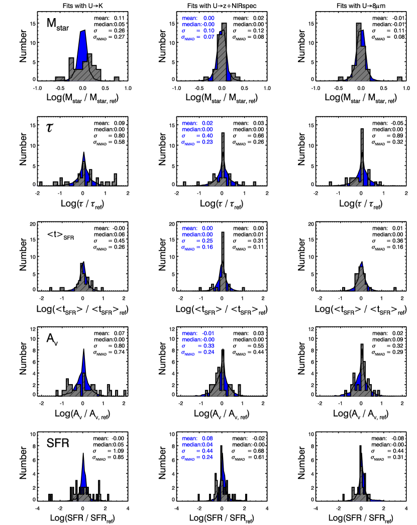
Figure 13.— Left Panels: Comparison of stellar population parameters determined using only the broadband U$\rightarrow$K photometry to those determined using all of the data (U$\rightarrow$8$\micron$+NIRspec). Middle Panels: As the left panels, but comparing parameters from broadband plus NIR spectroscopy (U$\rightarrow$z^′+NIRspec) to those determined with U$\rightarrow$8$\micron$+NIRspec. Right Panels: As left panels but comparing parameters from broadband optical and IRAC photometry (U$\rightarrow$8$\micron$) to those determined with U$\rightarrow$8$\micron$+NIRspec. The blue curves in each panel are the spread in the distribution that would be expected based on the Monte Carlo errors determined using the U$\rightarrow$8$\micron$+NIRspec data. If the parameters determined from a subset of the data have the same accuracy and precision as those determined from the entire U$\rightarrow$8$\micron$+NIRspec data set, the blue and grey histograms should be similar. The differences in the accuracy of the parameters using the various datasets can be determined by comparing the $\sigma$ or the $\sigma_{\mbox{\scriptsize NMAD}}$ accross the different datasets. The addition of rest-frame NIR data from IRAC provides significant improvement in most parameters, particularly compared to those determined from U$\rightarrow$K photometry alone. The IRAC data provides better constraints than the NIR spectroscopy on the parameters M${}_{\mbox{\scriptsize star}}$, A_v, and SFR; whereas the NIR spectroscopy provides better constraints on $\tau$ and $\langle t\rangle_{\mbox{\scriptsize SFR}}$.

The standard deviation ($\sigma$) of the distributions are listed in the upper right of each panel in Figure 13. These serve as an indication of the scatter between the best fit parameters, even though some of the distributions are non-Gaussian. Standard deviations are sensitive to large outliers and therefore we also compute the normalized median absolute deviation ($\sigma_{\mbox{\scriptsize NMAD}}$) to compare if the $\sigma$ is representative of the true scatter in parameters or is dominated by a few large outliers. For a Gaussian error distribution, $\sigma_{\mbox{\scriptsize NMAD}}$ = rms.
Because the histograms are ratios of parameters computed with different datasets, the scatter is caused by the combination of errors in both datasets. To determine whether the given data improves the quality of the fits we must assess how much of the scatter is caused by uncertainties in U$\rightarrow$K, U$\rightarrow$z^′+NIRspec, or U$\rightarrow$8$\micron$ fits and how much is intrinsic to the SED fitting with the comparison sample (U$\rightarrow$8$\micron$+NIRspec). The intrinsic contribution is estimated by simulating a new distribution of the U$\rightarrow$8$\micron$+NIRspec fit parameters based on the error estimates listed in Table 1. We generate this distribution by drawing 200 new values of each parameter, for each galaxy, using the uncertainties and compare the new parameters to the original ones. The resulting “expected” distributions are plotted in blue in Figure 13 with the measured mean, median, $\sigma$ and $\sigma_{\mbox{\scriptsize NMAD}}$ also listed in blue. These values are the scatters used on the X-axis of Figure 13. Where the grey and blue histograms differ in mean, median, or sigma, the IRAC data provides additional constraints. The main results from the histograms in Figure 13 are summarized in $\S$ 4.3 and $\S$ 4.4.

Table 1SED Modeling Parameters

Name	Model	$z$	age	$\tau$	Av	M∗	SFR	$<t_{SFR}>$	$<\chi_{r}^{2}>$
			Gyr	Gyr	mag	1011M⊙	$M_{\odot}$ yr-1	Gyr
(1)	(2)	(3)	(4)	(5)	(6)	(7)	(8)	(9)
1030-32	BC03 (no irac)	2.23${}^{+0.13}_{-0.02}$	1.00${}^{+0.00}_{-0.20}$	0.01${}^{+0.09}_{-0.00}$	0.1${}^{+0.4}_{-0.1}$	1.34${}^{+0.30}_{-0.24}$	0.0${}^{+0.0}_{-0.0}$	0.99${}^{+0.00}_{-0.21}$	1.56
…	BC03	2.23${}^{+0.13}_{-0.03}$	0.90${}^{+0.60}_{-0.20}$	0.03${}^{+0.12}_{-0.02}$	0.4${}^{+0.3}_{-0.4}$	1.63${}^{+0.25}_{-0.25}$	0.0${}^{+0.5}_{-0.0}$	0.87${}^{+0.60}_{-0.20}$	1.46
…	MAR05 (no irac)	2.23${}^{+0.13}_{-0.03}$	1.00${}^{+0.25}_{-0.20}$	0.05${}^{+0.10}_{-0.04}$	0.0${}^{+0.1}_{-0.0}$	1.16${}^{+0.12}_{-0.20}$	9.6${}^{+0.2}_{-9.6}$	0.95${}^{+0.15}_{-0.18}$	1.92
…	MAR05	2.23${}^{+0.02}_{-0.14}$	0.90${}^{+2.10}_{-0.10}$	0.01${}^{+0.39}_{-0.00}$	0.0${}^{+0.0}_{-0.0}$	1.05${}^{+1.44}_{-0.13}$	0.0${}^{+0.4}_{-0.0}$	0.89${}^{+1.71}_{-0.13}$	1.89
…	CB08 (no irac)	2.36${}^{+0.00}_{-0.14}$	0.90${}^{+0.10}_{-0.20}$	0.01${}^{+0.09}_{-0.00}$	0.1${}^{+0.4}_{-0.1}$	1.46${}^{+0.41}_{-0.24}$	0.0${}^{+0.0}_{-0.0}$	0.89${}^{+0.10}_{-0.20}$	1.55
…	CB08	2.36${}^{+0.00}_{-0.14}$	0.90${}^{+0.10}_{-0.00}$	0.01${}^{+0.07}_{-0.00}$	0.0${}^{+0.0}_{-0.0}$	1.30${}^{+0.11}_{-0.05}$	0.0${}^{+0.0}_{-0.0}$	0.89${}^{+0.10}_{-0.04}$	1.48
1030-101	BC03 (no irac)	1.79${}^{+0.07}_{-0.12}$	0.40${}^{+1.85}_{-0.10}$	0.02${}^{+0.27}_{-0.01}$	1.8${}^{+0.3}_{-1.3}$	2.76${}^{+0.62}_{-0.54}$	0.0${}^{+13.5}_{-0.0}$	0.37${}^{+1.32}_{-0.09}$	0.74
…	BC03	1.79${}^{+0.07}_{-0.09}$	0.40${}^{+0.40}_{-0.10}$	0.04${}^{+0.08}_{-0.03}$	1.9${}^{+0.2}_{-0.4}$	2.91${}^{+0.54}_{-0.49}$	0.4${}^{+10.6}_{-0.4}$	0.36${}^{+0.16}_{-0.08}$	0.82
…	MAR05 (no irac)	1.72${}^{+0.20}_{-0.06}$	1.00${}^{+1.75}_{-0.80}$	0.12${}^{+0.28}_{-0.11}$	0.6${}^{+1.7}_{-0.4}$	1.45${}^{+1.22}_{-0.44}$	0.3${}^{+11.5}_{-0.3}$	0.88${}^{+1.47}_{-0.70}$	0.84
…	MAR05	1.79${}^{+0.08}_{-0.09}$	0.70${}^{+0.30}_{-0.40}$	0.04${}^{+0.11}_{-0.03}$	0.7${}^{+1.1}_{-0.3}$	1.49${}^{+0.81}_{-0.18}$	0.0${}^{+2.3}_{-0.0}$	0.66${}^{+0.33}_{-0.38}$	0.89
…	CB08 (no irac)	1.72${}^{+0.12}_{-0.04}$	0.90${}^{+2.60}_{-0.50}$	0.12${}^{+0.38}_{-0.11}$	1.1${}^{+0.7}_{-1.0}$	2.10${}^{+0.93}_{-0.70}$	1.2${}^{+6.5}_{-1.2}$	0.78${}^{+2.22}_{-0.43}$	0.80
…	CB08	1.72${}^{+0.12}_{-0.04}$	0.80${}^{+1.45}_{-0.30}$	0.10${}^{+0.20}_{-0.09}$	1.2${}^{+0.3}_{-0.9}$	2.14${}^{+0.45}_{-0.82}$	0.9${}^{+6.6}_{-0.9}$	0.70${}^{+1.25}_{-0.22}$	0.81
1030-609	BC03 (no irac)	1.800	0.90${}^{+1.60}_{-0.85}$	10.0${}^{+10.0}_{-9.99}$	1.5${}^{+0.4}_{-0.3}$	0.88${}^{+0.42}_{-0.47}$	118.2${}^{+156.5}_{-105.2}$	0.45${}^{+0.81}_{-0.41}$	1.09
…	BC03	1.800	0.90${}^{+1.35}_{-0.70}$	10.0${}^{+10.0}_{-9.88}$	1.5${}^{+0.3}_{-0.3}$	0.88${}^{+0.36}_{-0.31}$	118.2${}^{+100.6}_{-53.1}$	0.45${}^{+0.71}_{-0.30}$	1.12
…	MAR05 (no irac)	1.800	0.60${}^{+0.30}_{-0.55}$	20.0${}^{+0.00}_{-19.9}$	1.5${}^{+0.6}_{-0.2}$	0.70${}^{+0.05}_{-0.39}$	140.6${}^{+396.2}_{-57.2}$	0.30${}^{+0.16}_{-0.26}$	1.12
…	MAR05	1.800	0.10${}^{+0.40}_{-0.05}$	0.12${}^{+19.8}_{-0.09}$	1.9${}^{+0.1}_{-0.4}$	0.41${}^{+0.23}_{-0.08}$	303.8${}^{+126.0}_{-169.3}$	0.05${}^{+0.20}_{-0.02}$	1.19
…	CB08 (no irac)	1.800	0.80${}^{+0.70}_{-0.60}$	5.00${}^{+15.0}_{-4.90}$	1.5${}^{+0.3}_{-0.3}$	0.82${}^{+0.24}_{-0.24}$	118.4${}^{+104.2}_{-56.4}$	0.41${}^{+0.41}_{-0.28}$	1.02
…	CB08	1.800	0.10${}^{+0.00}_{-0.04}$	0.04${}^{+0.01}_{-0.03}$	1.8${}^{+0.0}_{-0.2}$	0.50${}^{+0.01}_{-0.09}$	131.8${}^{+32.6}_{-118.9}$	0.06${}^{+0.00}_{-0.01}$	1.23
1030-807	BC03 (no irac)	2.367	0.70${}^{+0.20}_{-0.20}$	0.12${}^{+0.03}_{-0.04}$	0.2${}^{+0.3}_{-0.2}$	1.11${}^{+0.17}_{-0.12}$	3.6${}^{+1.8}_{-2.4}$	0.58${}^{+0.17}_{-0.08}$	1.87
…	BC03	2.367	0.50${}^{+0.30}_{-0.30}$	0.10${}^{+0.05}_{-0.09}$	0.8${}^{+0.5}_{-0.4}$	1.47${}^{+0.22}_{-0.25}$	12.9${}^{+14.3}_{-12.9}$	0.40${}^{+0.25}_{-0.23}$	1.88
…	MAR05 (no irac)	2.367	0.60${}^{+0.10}_{-0.54}$	0.08${}^{+0.04}_{-0.07}$	0.0${}^{+1.8}_{-0.0}$	0.82${}^{+0.30}_{-1.52}$	0.7${}^{+28.4}_{-0.1}$	0.52${}^{+0.06}_{-0.47}$	1.97
…	MAR05	2.367	0.60${}^{+0.10}_{-0.51}$	0.08${}^{+0.04}_{-0.07}$	0.0${}^{+1.5}_{-0.0}$	0.82${}^{+0.30}_{-0.00}$	0.7${}^{+2.1}_{-0.1}$	0.52${}^{+0.06}_{-0.44}$	1.78
…	CB08 (no irac)	2.367	0.70${}^{+0.20}_{-0.20}$	0.12${}^{+0.03}_{-0.04}$	0.2${}^{+0.6}_{-0.2}$	1.11${}^{+0.34}_{-0.14}$	3.6${}^{+9.1}_{-2.7}$	0.58${}^{+0.17}_{-0.17}$	1.87
…	CB08	2.367	0.70${}^{+0.20}_{-0.10}$	0.12${}^{+0.03}_{-0.04}$	0.2${}^{+0.0}_{-0.2}$	1.10${}^{+0.00}_{-0.13}$	3.6${}^{+0.0}_{-2.6}$	0.58${}^{+0.17}_{-0.06}$	1.74
1030-1531	BC03 (no irac)	2.613	0.50${}^{+0.50}_{-0.00}$	0.20${}^{+0.80}_{-0.00}$	0.4${}^{+0.2}_{-0.1}$	1.43${}^{+0.70}_{-0.00}$	81.0${}^{+69.7}_{-28.4}$	0.34${}^{+0.24}_{-0.00}$	1.38
…	BC03	2.613	2.50${}^{+0.00}_{-0.75}$	10.0${}^{+10.0}_{-7.50}$	0.6${}^{+0.1}_{-0.0}$	3.29${}^{+0.40}_{-0.48}$	153.5${}^{+38.0}_{-3.7}$	1.30${}^{+0.05}_{-0.33}$	1.81
…	MAR05 (no irac)	2.613	0.40${}^{+0.60}_{-0.10}$	0.25${}^{+9.75}_{-0.15}$	0.6${}^{+0.1}_{-0.2}$	1.30${}^{+0.57}_{-0.21}$	160.2${}^{+61.4}_{-90.2}$	0.25${}^{+0.25}_{-0.03}$	1.58
…	MAR05	2.613	0.90${}^{+0.10}_{-0.20}$	2.50${}^{+17.5}_{-1.85}$	0.7${}^{+0.0}_{-0.1}$	1.91${}^{+0.17}_{-0.23}$	219.1${}^{+3.3}_{-48.6}$	0.47${}^{+0.05}_{-0.09}$	1.60
…	CB08 (no irac)	2.613	0.50${}^{+0.50}_{-0.00}$	0.20${}^{+0.80}_{-0.00}$	0.4${}^{+0.2}_{-0.1}$	1.43${}^{+0.70}_{-0.00}$	81.0${}^{+69.7}_{-28.5}$	0.34${}^{+0.24}_{-0.00}$	1.39
…	CB08	2.613	1.00${}^{+0.50}_{-0.30}$	0.90${}^{+1.60}_{-0.50}$	0.6${}^{+0.0}_{-0.1}$	2.14${}^{+0.27}_{-0.40}$	149.7${}^{+4.3}_{-33.3}$	0.59${}^{+0.24}_{-0.16}$	1.36
1030-1611	BC03 (no irac)	1.93${}^{+0.14}_{-0.15}$	0.50${}^{+1.50}_{-0.30}$	0.12${}^{+0.28}_{-0.11}$	1.8${}^{+0.5}_{-1.1}$	1.92${}^{+0.57}_{-0.55}$	32.4${}^{+81.9}_{-32.4}$	0.38${}^{+0.98}_{-0.21}$	0.75
…	BC03	1.93${}^{+0.04}_{-0.25}$	0.90${}^{+2.60}_{-0.40}$	0.20${}^{+0.60}_{-0.12}$	1.2${}^{+0.4}_{-0.9}$	1.72${}^{+1.34}_{-0.39}$	12.6${}^{+8.7}_{-10.6}$	0.71${}^{+2.15}_{-0.30}$	0.81
…	MAR05 (no irac)	1.93${}^{+0.14}_{-0.13}$	0.70${}^{+0.80}_{-0.65}$	0.12${}^{+0.18}_{-0.11}$	0.7${}^{+1.9}_{-0.5}$	0.98${}^{+0.82}_{-0.18}$	3.1${}^{+123.6}_{-3.1}$	0.58${}^{+0.67}_{-0.51}$	0.75
…	MAR05	1.93${}^{+0.14}_{-0.25}$	0.30${}^{+3.20}_{-0.22}$	0.03${}^{+0.87}_{-0.02}$	1.4${}^{+0.8}_{-1.3}$	1.19${}^{+1.67}_{-0.43}$	0.2${}^{+67.3}_{-0.2}$	0.27${}^{+2.47}_{-0.19}$	0.73
…	CB08 (no irac)	1.93${}^{+0.14}_{-0.14}$	0.60${}^{+1.65}_{-0.40}$	0.12${}^{+0.28}_{-0.11}$	1.5${}^{+0.7}_{-1.1}$	1.63${}^{+0.58}_{-0.41}$	12.2${}^{+60.9}_{-12.2}$	0.48${}^{+0.72}_{-0.23}$	0.77
…	CB08	1.69${}^{+0.27}_{-0.00}$	3.50${}^{+0.00}_{-2.50}$	0.65${}^{+0.05}_{-0.45}$	0.3${}^{+0.5}_{-0.3}$	1.62${}^{+0.32}_{-0.68}$	1.5${}^{+2.6}_{-0.9}$	2.86${}^{+0.04}_{-2.05}$	0.96
1030-1839	BC03 (no irac)	2.312	2.25${}^{+0.50}_{-1.55}$	2.00${}^{+18.0}_{-1.75}$	1.1${}^{+0.3}_{-0.3}$	2.94${}^{+0.77}_{-1.36}$	94.1${}^{+93.1}_{-51.3}$	1.33${}^{+0.44}_{-0.85}$	2.74
…	BC03	2.312	0.80${}^{+0.20}_{-0.40}$	0.25${}^{+0.15}_{-0.15}$	0.7${}^{+0.3}_{-0.2}$	1.50${}^{+0.19}_{-0.35}$	32.9${}^{+37.4}_{-13.5}$	0.58${}^{+0.15}_{-0.28}$	2.73
…	MAR05 (no irac)	2.312	1.50${}^{+1.25}_{-1.10}$	2.75${}^{+17.2}_{-2.63}$	1.2${}^{+0.3}_{-0.5}$	2.14${}^{+0.91}_{-1.05}$	136.4${}^{+133.7}_{-100.6}$	0.81${}^{+0.58}_{-0.57}$	2.71
…	MAR05	2.312	0.30${}^{+0.10}_{-0.10}$	0.08${}^{+0.04}_{-0.03}$	1.0${}^{+0.3}_{-0.7}$	1.15${}^{+0.00}_{-0.36}$	43.0${}^{+88.5}_{-34.7}$	0.22${}^{+0.09}_{-0.08}$	2.74
…	CB08 (no irac)	2.312	2.25${}^{+0.50}_{-1.65}$	2.00${}^{+18.0}_{-1.80}$	1.1${}^{+0.3}_{-0.3}$	2.94${}^{+0.78}_{-1.40}$	93.8${}^{+94.5}_{-51.2}$	1.33${}^{+0.44}_{-0.90}$	2.74
…	CB08	2.312	0.60${}^{+0.20}_{-0.10}$	0.12${}^{+0.08}_{-0.02}$	0.3${}^{+0.2}_{-0.3}$	0.92${}^{+0.30}_{-0.17}$	6.8${}^{+14.8}_{-4.3}$	0.48${}^{+0.13}_{-0.09}$	3.01
1030-2026	BC03 (no irac)	2.511	1.00${}^{+0.50}_{-0.30}$	0.20${}^{+0.05}_{-0.05}$	0.7${}^{+0.4}_{-0.7}$	3.01${}^{+0.50}_{-1.07}$	13.6${}^{+14.2}_{-11.0}$	0.80${}^{+0.44}_{-0.25}$	1.46
…	BC03	2.511	0.80${}^{+0.20}_{-0.30}$	0.20${}^{+0.05}_{-0.08}$	1.2${}^{+0.3}_{-0.2}$	3.70${}^{+0.46}_{-0.41}$	44.8${}^{+33.0}_{-19.1}$	0.61${}^{+0.15}_{-0.22}$	1.77
…	MAR05 (no irac)	2.511	0.90${}^{+0.00}_{-0.20}$	0.15${}^{+0.00}_{-0.03}$	0.2${}^{+0.3}_{-0.1}$	1.80${}^{+0.31}_{-0.25}$	3.8${}^{+4.9}_{-1.7}$	0.75${}^{+0.00}_{-0.17}$	1.58
…	MAR05	2.511	0.80${}^{+0.10}_{-0.10}$	0.15${}^{+0.00}_{-0.03}$	0.5${}^{+0.0}_{-0.3}$	2.10${}^{+6.10}_{-0.27}$	8.7${}^{+0.0}_{-4.8}$	0.65${}^{+0.09}_{-0.07}$	1.81
…	CB08 (no irac)	2.511	1.00${}^{+0.50}_{-0.30}$	0.20${}^{+0.05}_{-0.05}$	0.7${}^{+0.3}_{-0.5}$	2.99${}^{+0.50}_{-0.80}$	13.5${}^{+12.1}_{-9.9}$	0.80${}^{+0.44}_{-0.25}$	1.44
…	CB08	2.511	0.80${}^{+0.20}_{-0.10}$	0.15${}^{+0.05}_{-0.00}$	0.7${}^{+0.2}_{-0.1}$	2.55${}^{+0.39}_{--3.0}$	10.8${}^{+11.2}_{-0.0}$	0.65${}^{+0.15}_{-0.09}$	1.66
1030-2329	BC03 (no irac)	2.236	0.80${}^{+0.20}_{-0.60}$	0.15${}^{+0.05}_{-0.14}$	0.7${}^{+1.2}_{-0.6}$	1.54${}^{+0.38}_{-0.40}$	6.5${}^{+32.0}_{-6.5}$	0.65${}^{+0.19}_{-0.49}$	1.38
…	BC03	2.236	0.80${}^{+0.20}_{-0.50}$	0.15${}^{+0.05}_{-0.14}$	0.7${}^{+0.6}_{-0.1}$	1.55${}^{+0.23}_{-0.24}$	6.5${}^{+8.3}_{-6.5}$	0.65${}^{+0.15}_{-0.38}$	1.29
…	MAR05 (no irac)	2.236	0.70${}^{+0.10}_{-0.10}$	0.10${}^{+0.02}_{-0.02}$	0.1${}^{+0.3}_{-0.1}$	0.86${}^{+0.10}_{-0.08}$	1.0${}^{+0.2}_{-0.2}$	0.60${}^{+0.08}_{-0.08}$	1.25
…	MAR05	2.236	0.70${}^{+0.10}_{-0.20}$	0.10${}^{+0.02}_{-0.09}$	0.1${}^{+0.2}_{-0.1}$	0.85${}^{+0.05}_{-0.11}$	1.0${}^{+0.2}_{-1.0}$	0.60${}^{+0.08}_{-0.14}$	1.13
…	CB08 (no irac)	2.236	0.70${}^{+0.30}_{-0.50}$	0.12${}^{+0.08}_{-0.11}$	0.6${}^{+1.2}_{-0.3}$	1.32${}^{+0.59}_{-0.19}$	4.3${}^{+27.9}_{-4.3}$	0.58${}^{+0.22}_{-0.41}$	1.38
…	CB08	2.236	0.80${}^{+0.20}_{-0.10}$	0.12${}^{+0.03}_{-0.02}$	0.3${}^{+0.2}_{-0.3}$	1.12${}^{+0.16}_{-0.10}$	1.5${}^{+2.2}_{-0.3}$	0.68${}^{+0.17}_{-0.09}$	1.33
1030-2559	BC03 (no irac)	2.25${}^{+0.19}_{-0.04}$	0.90${}^{+0.60}_{-0.50}$	0.12${}^{+0.08}_{-0.11}$	0.6${}^{+0.7}_{-0.6}$	1.84${}^{+0.70}_{-0.51}$	1.1${}^{+6.8}_{-1.1}$	0.78${}^{+0.52}_{-0.30}$	1.39
…	BC03	2.25${}^{+0.19}_{-0.04}$	0.70${}^{+0.80}_{-0.20}$	0.08${}^{+0.12}_{-0.07}$	0.8${}^{+0.4}_{-0.6}$	1.92${}^{+0.37}_{-0.37}$	0.5${}^{+4.4}_{-0.5}$	0.62${}^{+0.68}_{-0.16}$	1.26
…	MAR05 (no irac)	2.30${}^{+0.08}_{-0.08}$	0.90${}^{+0.60}_{-0.30}$	0.10${}^{+0.10}_{-0.09}$	0.0${}^{+0.5}_{-0.0}$	1.13${}^{+0.40}_{-0.13}$	0.1${}^{+0.6}_{-0.1}$	0.80${}^{+0.50}_{-0.22}$	1.57
…	MAR05	2.30${}^{+0.14}_{-0.08}$	0.90${}^{+0.60}_{-0.20}$	0.10${}^{+0.10}_{-0.09}$	0.0${}^{+0.2}_{-0.0}$	1.12${}^{+0.43}_{-0.15}$	0.1${}^{+0.5}_{-0.1}$	0.80${}^{+0.50}_{-0.15}$	1.47
…	CB08 (no irac)	2.30${}^{+0.14}_{-0.06}$	0.80${}^{+0.70}_{-0.30}$	0.10${}^{+0.10}_{-0.09}$	0.6${}^{+0.6}_{-0.6}$	1.83${}^{+0.80}_{-0.40}$	0.8${}^{+4.6}_{-0.8}$	0.70${}^{+0.60}_{-0.22}$	1.39
…	CB08	2.30${}^{+0.17}_{-0.06}$	1.00${}^{+0.00}_{-0.30}$	0.12${}^{+0.00}_{-0.11}$	0.2${}^{+0.3}_{-0.2}$	1.49${}^{+0.14}_{-0.33}$	0.4${}^{+0.5}_{-0.4}$	0.88${}^{+0.09}_{-0.23}$	1.32
1030-2728	BC03 (no irac)	2.504	0.50${}^{+0.10}_{-0.20}$	0.08${}^{+0.02}_{-0.07}$	0.8${}^{+0.4}_{-0.3}$	1.93${}^{+0.47}_{-0.34}$	6.1${}^{+15.0}_{-6.1}$	0.42${}^{+0.09}_{-0.15}$	1.93
…	BC03	2.504	0.20${}^{+0.20}_{-0.00}$	0.02${}^{+0.06}_{-0.01}$	1.6${}^{+0.1}_{-0.3}$	2.48${}^{+0.27}_{-0.11}$	0.7${}^{+29.1}_{-0.7}$	0.18${}^{+0.14}_{-0.00}$	1.94
…	MAR05 (no irac)	2.504	0.30${}^{+0.30}_{-0.10}$	0.02${}^{+0.05}_{-0.01}$	0.9${}^{+0.5}_{-0.6}$	1.70${}^{+0.48}_{-0.51}$	0.0${}^{+10.9}_{-0.0}$	0.27${}^{+0.24}_{-0.09}$	2.04
…	MAR05	2.504	0.40${}^{+0.10}_{-0.00}$	0.05${}^{+0.03}_{-0.04}$	0.6${}^{+0.1}_{-0.2}$	1.49${}^{+0.15}_{-0.19}$	1.2${}^{+3.8}_{-1.2}$	0.35${}^{+0.07}_{-0.00}$	1.96
…	CB08 (no irac)	2.504	0.50${}^{+0.10}_{-0.20}$	0.08${}^{+0.02}_{-0.07}$	0.8${}^{+0.4}_{-0.3}$	1.93${}^{+0.22}_{-0.34}$	6.1${}^{+0.7}_{-6.1}$	0.42${}^{+0.09}_{-0.14}$	1.93
…	CB08	2.504	0.50${}^{+0.10}_{-0.10}$	0.08${}^{+0.02}_{-0.06}$	0.8${}^{+0.1}_{-0.1}$	1.92${}^{+0.08}_{-0.32}$	6.1${}^{+0.6}_{-6.1}$	0.42${}^{+0.08}_{-0.07}$	1.76
1030-2927	BC03 (no irac)	1.83${}^{+0.14}_{-0.13}$	0.40${}^{+0.85}_{-0.31}$	0.12${}^{+0.28}_{-0.11}$	1.4${}^{+0.4}_{-1.3}$	1.05${}^{+0.37}_{-0.28}$	41.0${}^{+52.3}_{-41.0}$	0.29${}^{+0.71}_{-0.20}$	1.20
…	BC03	1.83${}^{+0.11}_{-0.14}$	0.40${}^{+0.60}_{-0.30}$	0.12${}^{+0.28}_{-0.11}$	1.4${}^{+0.4}_{-0.7}$	1.05${}^{+0.37}_{-0.26}$	41.0${}^{+30.4}_{-40.8}$	0.29${}^{+0.47}_{-0.20}$	1.14
…	MAR05 (no irac)	1.84${}^{+0.09}_{-0.07}$	0.20${}^{+0.10}_{-0.15}$	0.04${}^{+0.04}_{-0.03}$	1.3${}^{+0.6}_{-0.4}$	0.83${}^{+0.12}_{-0.29}$	17.3${}^{+77.8}_{-17.0}$	0.16${}^{+0.08}_{-0.10}$	1.06
…	MAR05	1.83${}^{+0.12}_{-0.08}$	0.10${}^{+0.20}_{-0.05}$	0.02${}^{+0.07}_{-0.01}$	1.8${}^{+0.2}_{-0.5}$	0.74${}^{+0.22}_{-0.23}$	65.8${}^{+58.7}_{-64.7}$	0.07${}^{+0.15}_{-0.03}$	1.08
…	CB08 (no irac)	1.83${}^{+0.14}_{-0.13}$	0.10${}^{+0.90}_{-0.01}$	0.01${}^{+0.24}_{-0.00}$	1.7${}^{+0.2}_{-1.5}$	0.79${}^{+0.32}_{-0.07}$	0.4${}^{+39.6}_{-0.0}$	0.09${}^{+0.71}_{-0.00}$	1.32
…	CB08	1.83${}^{+0.12}_{-0.14}$	0.10${}^{+0.90}_{-0.01}$	0.01${}^{+0.24}_{-0.00}$	1.7${}^{+0.0}_{-1.5}$	0.79${}^{+0.25}_{-0.04}$	0.4${}^{+11.3}_{-0.0}$	0.09${}^{+0.71}_{-0.00}$	1.23
1256-0	BC03 (no irac)	2.29${}^{+0.20}_{-0.18}$	0.20${}^{+1.30}_{-0.00}$	0.01${}^{+0.24}_{-0.00}$	1.9${}^{+0.3}_{-1.8}$	4.12${}^{+1.29}_{-1.51}$	0.0${}^{+194.9}_{-0.0}$	0.19${}^{+1.11}_{-0.02}$	1.12
…	BC03	2.29${}^{+0.15}_{-0.21}$	0.70${}^{+1.30}_{-0.40}$	0.12${}^{+0.18}_{-0.11}$	1.0${}^{+0.5}_{-0.8}$	3.62${}^{+1.84}_{-0.70}$	11.9${}^{+23.4}_{-11.9}$	0.58${}^{+0.87}_{-0.31}$	1.06
…	MAR05 (no irac)	2.29${}^{+0.18}_{-0.03}$	0.70${}^{+0.30}_{-0.61}$	0.10${}^{+0.05}_{-0.09}$	0.4${}^{+1.7}_{-0.4}$	2.13${}^{+1.85}_{-0.55}$	2.6${}^{+19.5}_{-2.6}$	0.60${}^{+0.27}_{-0.41}$	0.98
…	MAR05	2.29${}^{+0.18}_{-0.03}$	0.90${}^{+0.35}_{-0.80}$	0.12${}^{+0.08}_{-0.11}$	0.1${}^{+1.9}_{-0.1}$	1.93${}^{+1.81}_{-0.42}$	1.1${}^{+16.6}_{-1.1}$	0.78${}^{+0.09}_{-0.69}$	0.93
…	CB08 (no irac)	2.29${}^{+0.20}_{-0.03}$	0.60${}^{+0.90}_{-0.40}$	0.10${}^{+0.10}_{-0.09}$	1.2${}^{+1.0}_{-1.1}$	3.60${}^{+1.33}_{-1.03}$	12.1${}^{+101.3}_{-12.1}$	0.50${}^{+0.55}_{-0.34}$	1.11
…	CB08	2.29${}^{+0.20}_{-0.20}$	1.00${}^{+1.75}_{-0.40}$	0.15${}^{+0.25}_{-0.14}$	0.4${}^{+0.3}_{-0.4}$	2.72${}^{+1.94}_{-0.66}$	3.1${}^{+3.1}_{-3.1}$	0.85${}^{+1.50}_{-0.25}$	1.15
1256-142	BC03 (no irac)	2.24${}^{+0.12}_{-0.04}$	2.25${}^{+0.75}_{-1.85}$	0.30${}^{+0.10}_{-0.29}$	0.1${}^{+1.3}_{-0.1}$	2.76${}^{+1.25}_{-0.96}$	0.7${}^{+9.2}_{-0.7}$	1.95${}^{+0.65}_{-1.57}$	1.19
…	BC03	2.24${}^{+0.19}_{-0.04}$	1.75${}^{+0.75}_{-1.05}$	0.25${}^{+0.05}_{-0.24}$	0.2${}^{+0.5}_{-0.2}$	2.47${}^{+0.63}_{-0.90}$	1.2${}^{+1.5}_{-1.2}$	1.50${}^{+0.69}_{-0.81}$	1.20
…	MAR05 (no irac)	2.24${}^{+0.03}_{-0.03}$	1.50${}^{+1.25}_{-0.80}$	0.20${}^{+0.20}_{-0.19}$	0.1${}^{+0.5}_{-0.1}$	1.76${}^{+0.96}_{-0.33}$	0.6${}^{+1.9}_{-0.6}$	1.30${}^{+1.05}_{-0.64}$	1.27
…	MAR05	2.24${}^{+0.02}_{-0.04}$	1.75${}^{+1.25}_{-0.25}$	0.25${}^{+0.15}_{-0.05}$	0.0${}^{+0.0}_{-0.0}$	1.90${}^{+1.00}_{-0.35}$	0.9${}^{+0.1}_{-0.5}$	1.50${}^{+1.10}_{-0.20}$	1.39
…	CB08 (no irac)	2.24${}^{+0.03}_{-0.03}$	1.50${}^{+1.25}_{-1.00}$	0.20${}^{+0.20}_{-0.19}$	0.4${}^{+0.9}_{-0.4}$	2.32${}^{+1.35}_{-0.71}$	0.9${}^{+8.9}_{-0.9}$	1.30${}^{+1.05}_{-0.73}$	1.10
…	CB08	2.42${}^{+0.02}_{-0.19}$	1.00${}^{+0.00}_{-0.20}$	0.10${}^{+0.02}_{-0.09}$	0.0${}^{+0.1}_{-0.0}$	1.61${}^{+0.31}_{-0.04}$	0.1${}^{+0.3}_{-0.1}$	0.90${}^{+0.08}_{-0.05}$	1.62
1256-519	BC03 (no irac)	1.857	0.30${}^{+1.70}_{-0.23}$	0.12${}^{+19.8}_{-0.11}$	3.2${}^{+0.2}_{-0.7}$	4.80${}^{+2.68}_{-1.76}$	444.7${}^{+946.1}_{-442.6}$	0.20${}^{+0.82}_{-0.14}$	1.25
…	BC03	1.857	2.50${}^{+1.00}_{-0.75}$	0.40${}^{+0.20}_{-0.39}$	0.9${}^{+0.3}_{-0.2}$	4.64${}^{+0.78}_{-0.60}$	3.0${}^{+2.7}_{-3.0}$	2.10${}^{+0.89}_{-0.64}$	2.55
…	MAR05 (no irac)	1.857	0.60${}^{+0.65}_{-0.56}$	0.15${}^{+19.8}_{-0.14}$	2.2${}^{+1.5}_{-0.6}$	3.51${}^{+1.46}_{-1.40}$	55.9${}^{+252}_{-55.9}$	0.46${}^{+0.44}_{-0.43}$	1.25
…	MAR05	1.857	3.50${}^{+0.00}_{-3.30}$	0.65${}^{+0.05}_{-0.64}$	0.9${}^{+1.5}_{-0.1}$	5.09${}^{+0.34}_{-1.69}$	4.8${}^{+2.1}_{-4.8}$	2.86${}^{+0.04}_{-2.67}$	2.33
…	CB08 (no irac)	1.857	0.30${}^{+0.50}_{-0.23}$	0.10${}^{+0.80}_{-0.09}$	3.0${}^{+0.4}_{-0.3}$	4.24${}^{+1.30}_{-1.20}$	278.2${}^{+687.8}_{-276.0}$	0.21${}^{+0.25}_{-0.15}$	1.25
…	CB08	1.857	3.50${}^{+0.00}_{-0.25}$	0.50${}^{+0.00}_{-0.49}$	0.5${}^{+0.0}_{-0.1}$	4.44${}^{+0.43}_{-0.28}$	1.1${}^{+0.0}_{-1.1}$	3.00${}^{+0.48}_{-0.00}$	3.07
1256-1207	BC03 (no irac)	1.80${}^{+0.08}_{-0.16}$	0.80${}^{+0.95}_{-0.40}$	0.10${}^{+0.15}_{-0.09}$	0.7${}^{+0.7}_{-0.5}$	1.40${}^{+0.50}_{-0.22}$	0.6${}^{+5.4}_{-0.6}$	0.70${}^{+0.60}_{-0.32}$	1.06
…	BC03	1.66${}^{+0.19}_{-0.02}$	0.80${}^{+0.45}_{-0.40}$	0.12${}^{+0.08}_{-0.11}$	1.0${}^{+0.4}_{-0.5}$	1.35${}^{+0.18}_{-0.30}$	1.9${}^{+4.2}_{-1.9}$	0.68${}^{+0.37}_{-0.30}$	0.99
…	MAR05 (no irac)	1.80${}^{+0.08}_{-0.15}$	0.90${}^{+0.60}_{-0.30}$	0.10${}^{+0.10}_{-0.09}$	0.0${}^{+0.3}_{-0.0}$	0.78${}^{+0.24}_{-0.13}$	0.1${}^{+0.3}_{-0.1}$	0.80${}^{+0.50}_{-0.18}$	1.11
…	MAR05	1.80${}^{+0.09}_{-0.14}$	0.90${}^{+0.10}_{-0.70}$	0.10${}^{+0.02}_{-0.09}$	0.0${}^{+1.8}_{-0.0}$	0.78${}^{+0.85}_{-0.13}$	0.1${}^{+0.3}_{-0.1}$	0.80${}^{+0.09}_{-0.61}$	1.18
…	CB08 (no irac)	1.80${}^{+0.09}_{-0.15}$	0.80${}^{+0.20}_{-0.40}$	0.10${}^{+0.05}_{-0.09}$	0.6${}^{+0.5}_{-0.5}$	1.24${}^{+0.23}_{-0.28}$	0.5${}^{+1.4}_{-0.5}$	0.70${}^{+0.19}_{-0.25}$	0.97
…	CB08	1.80${}^{+0.08}_{-0.15}$	1.00${}^{+0.00}_{-0.30}$	0.12${}^{+0.03}_{-0.11}$	0.2${}^{+0.4}_{-0.1}$	1.04${}^{+0.41}_{-0.02}$	0.2${}^{+1.3}_{-0.2}$	0.88${}^{+0.10}_{-0.23}$	0.95
1256-1967	BC03 (no irac)	2.02${}^{+0.25}_{-0.18}$	0.10${}^{+0.00}_{-0.02}$	0.01${}^{+0.01}_{-0.00}$	1.8${}^{+0.2}_{-0.0}$	2.43${}^{+0.30}_{-0.25}$	1.4${}^{+103.2}_{-0.1}$	0.09${}^{+0.00}_{-0.01}$	3.24
…	BC03	2.02${}^{+0.25}_{-0.15}$	0.30${}^{+0.30}_{-0.10}$	0.02${}^{+0.06}_{-0.01}$	0.9${}^{+0.4}_{-0.7}$	1.96${}^{+0.28}_{-0.52}$	0.0${}^{+6.2}_{-0.0}$	0.28${}^{+0.24}_{-0.09}$	4.15
…	MAR05 (no irac)	2.27${}^{+0.00}_{-0.43}$	0.60${}^{+0.00}_{-0.55}$	0.08${}^{+0.00}_{-0.07}$	0.0${}^{+2.5}_{-0.0}$	1.85${}^{+1.15}_{-0.18}$	1.7${}^{+199}_{-1.5}$	0.52${}^{+0.00}_{-0.48}$	3.40
…	MAR05	1.99${}^{+0.04}_{-0.02}$	0.50${}^{+0.10}_{-0.20}$	0.05${}^{+0.03}_{-0.04}$	0.0${}^{+0.6}_{-0.0}$	1.22${}^{+0.47}_{-0.01}$	0.1${}^{+1.1}_{-0.1}$	0.45${}^{+0.07}_{-0.16}$	3.23
…	CB08 (no irac)	2.02${}^{+0.25}_{-0.18}$	0.10${}^{+0.00}_{-0.02}$	0.01${}^{+0.01}_{-0.00}$	1.8${}^{+0.2}_{-0.0}$	2.43${}^{+0.18}_{-0.35}$	1.4${}^{+98.3}_{-0.2}$	0.09${}^{+0.00}_{-0.01}$	3.24
…	CB08	2.02${}^{+0.25}_{-0.16}$	0.70${}^{+0.10}_{-0.60}$	0.10${}^{+0.02}_{-0.09}$	0.0${}^{+1.7}_{-0.0}$	1.57${}^{+0.62}_{-0.30}$	1.9${}^{+0.6}_{-1.9}$	0.60${}^{+0.00}_{-0.51}$	4.24
hdfs1-259	BC03 (no irac)	2.249	1.00${}^{+0.75}_{-0.70}$	5.00${}^{+15.0}_{-4.75}$	1.4${}^{+0.3}_{-0.2}$	2.10${}^{+0.67}_{-0.69}$	241.3${}^{+223.3}_{-94.6}$	0.51${}^{+0.38}_{-0.34}$	1.79
…	BC03	2.249	1.00${}^{+0.75}_{-0.70}$	5.00${}^{+15.0}_{-4.75}$	1.4${}^{+0.2}_{-0.2}$	2.10${}^{+0.53}_{-0.69}$	241.1${}^{+140.0}_{-93.0}$	0.51${}^{+0.40}_{-0.34}$	1.62
…	MAR05 (no irac)	2.249	0.30${}^{+0.40}_{-0.24}$	0.60${}^{+19.4}_{-0.57}$	1.6${}^{+0.3}_{-0.3}$	1.36${}^{+0.39}_{-0.58}$	417.0${}^{+492.2}_{-246.3}$	0.16${}^{+0.19}_{-0.12}$	1.78
…	MAR05	2.249	0.30${}^{+0.20}_{-0.25}$	20.0${}^{+0.00}_{-19.9}$	1.7${}^{+0.2}_{-0.3}$	1.38${}^{+0.15}_{-0.67}$	542.8${}^{+357.0}_{-280.1}$	0.15${}^{+0.10}_{-0.11}$	1.63
…	CB08 (no irac)	2.249	1.00${}^{+0.75}_{-0.70}$	5.00${}^{+15.0}_{-4.75}$	1.4${}^{+0.3}_{-0.2}$	2.10${}^{+0.58}_{-0.69}$	241.0${}^{+223.2}_{-93.3}$	0.51${}^{+0.37}_{-0.34}$	1.80
…	CB08	2.249	0.10${}^{+0.00}_{-0.04}$	0.04${}^{+0.01}_{-0.03}$	1.7${}^{+0.0}_{-0.2}$	1.10${}^{+0.04}_{-0.20}$	289.6${}^{+158.5}_{-261.1}$	0.06${}^{+0.00}_{-0.01}$	1.83
hdfs1-1849	BC03 (no irac)	2.30${}^{+0.06}_{-0.05}$	0.40${}^{+0.60}_{-0.20}$	0.08${}^{+0.17}_{-0.07}$	1.5${}^{+0.6}_{-0.7}$	2.97${}^{+1.41}_{-0.71}$	32.1${}^{+109.6}_{-32.1}$	0.32${}^{+0.48}_{-0.15}$	1.47
…	BC03	2.30${}^{+0.08}_{-0.05}$	0.40${}^{+0.60}_{-0.20}$	0.08${}^{+0.17}_{-0.07}$	1.6${}^{+0.3}_{-0.4}$	3.28${}^{+1.14}_{-0.63}$	35.5${}^{+84.3}_{-35.5}$	0.32${}^{+0.44}_{-0.15}$	1.34
…	MAR05 (no irac)	2.30${}^{+0.06}_{-0.05}$	0.40${}^{+0.50}_{-0.31}$	0.05${}^{+0.10}_{-0.04}$	0.9${}^{+1.1}_{-0.6}$	1.96${}^{+1.26}_{-0.45}$	1.7${}^{+64.9}_{-1.7}$	0.35${}^{+0.40}_{-0.26}$	1.43
…	MAR05	2.30${}^{+0.06}_{-0.05}$	0.40${}^{+0.50}_{-0.34}$	0.05${}^{+0.10}_{-0.04}$	0.9${}^{+1.4}_{-0.5}$	1.96${}^{+1.37}_{-0.40}$	1.7${}^{+157.7}_{-1.7}$	0.35${}^{+0.40}_{-0.27}$	1.33
…	CB08 (no irac)	2.30${}^{+0.06}_{-0.05}$	0.40${}^{+0.85}_{-0.20}$	0.08${}^{+0.17}_{-0.07}$	1.5${}^{+0.6}_{-0.8}$	2.96${}^{+1.52}_{-0.74}$	32.0${}^{+110.3}_{-32.0}$	0.32${}^{+0.68}_{-0.16}$	1.45
…	CB08	2.26${}^{+0.07}_{-0.03}$	0.80${}^{+0.20}_{-0.30}$	0.15${}^{+0.05}_{-0.07}$	0.9${}^{+0.2}_{-0.2}$	2.67${}^{+0.41}_{-0.45}$	11.3${}^{+12.1}_{-9.1}$	0.65${}^{+0.15}_{-0.23}$	1.39
hdfs2-509	BC03 (no irac)	2.918	0.60${}^{+0.00}_{-0.00}$	0.10${}^{+0.00}_{-0.00}$	0.1${}^{+0.0}_{-0.0}$	4.28${}^{+-6.1}_{-6.10}$	14.4${}^{+0.0}_{-0.0}$	0.50${}^{+0.00}_{-0.00}$	3.84
…	BC03	2.918	0.50${}^{+0.10}_{-0.00}$	0.10${}^{+0.02}_{-0.00}$	0.4${}^{+0.3}_{-0.3}$	5.20${}^{+1.44}_{-0.86}$	45.7${}^{+66.3}_{-31.1}$	0.40${}^{+0.09}_{-0.01}$	4.49
…	MAR05 (no irac)	2.918	0.40${}^{+0.10}_{-0.00}$	0.08${}^{+0.02}_{-0.00}$	0.4${}^{+0.0}_{-0.1}$	4.53${}^{+0.62}_{-0.00}$	48.0${}^{+0.0}_{-3.5}$	0.32${}^{+0.08}_{-0.00}$	5.13
…	MAR05	2.918	0.40${}^{+0.10}_{-0.00}$	0.08${}^{+0.02}_{-0.00}$	0.4${}^{+0.0}_{-0.2}$	4.51${}^{+-6.1}_{-0.31}$	47.9${}^{+0.0}_{-11.6}$	0.32${}^{+0.08}_{-0.00}$	4.69
…	CB08 (no irac)	2.918	0.60${}^{+0.00}_{-0.00}$	0.10${}^{+0.00}_{-0.00}$	0.1${}^{+0.0}_{-0.0}$	4.29${}^{+0.00}_{-0.00}$	14.3${}^{+0.0}_{-0.0}$	0.50${}^{+0.00}_{-0.00}$	3.87
…	CB08	2.918	0.60${}^{+0.00}_{-0.00}$	0.10${}^{+0.00}_{-0.00}$	0.1${}^{+0.0}_{-0.0}$	4.30${}^{+0.00}_{-0.00}$	14.4${}^{+0.0}_{-0.0}$	0.50${}^{+0.00}_{-0.00}$	3.56
hdfs2-1099	BC03 (no irac)	2.72${}^{+0.07}_{-0.24}$	0.80${}^{+0.20}_{-0.10}$	0.12${}^{+0.03}_{-0.02}$	0.2${}^{+0.5}_{-0.2}$	2.64${}^{+1.28}_{-0.58}$	3.7${}^{+12.9}_{-2.2}$	0.68${}^{+0.17}_{-0.09}$	1.46
…	BC03	2.51${}^{+0.24}_{-0.03}$	0.70${}^{+0.30}_{-0.20}$	0.12${}^{+0.08}_{-0.04}$	0.7${}^{+0.3}_{-0.3}$	3.09${}^{+0.62}_{-0.64}$	10.1${}^{+6.6}_{-6.4}$	0.58${}^{+0.22}_{-0.16}$	1.66
…	MAR05 (no irac)	2.72${}^{+0.06}_{-0.21}$	0.70${}^{+0.10}_{-0.00}$	0.10${}^{+0.02}_{-0.00}$	0.0${}^{+0.1}_{-0.0}$	2.04${}^{+0.36}_{-0.07}$	2.5${}^{+0.8}_{-0.0}$	0.60${}^{+0.08}_{-0.00}$	1.44
…	MAR05	2.55${}^{+0.10}_{-0.06}$	0.70${}^{+0.10}_{-0.00}$	0.10${}^{+0.02}_{-0.00}$	0.0${}^{+0.1}_{-0.0}$	1.68${}^{+0.34}_{--0.0}$	2.0${}^{+0.7}_{-0.0}$	0.60${}^{+0.08}_{-0.00}$	1.54
…	CB08 (no irac)	2.72${}^{+0.10}_{-0.24}$	0.80${}^{+0.20}_{-0.10}$	0.12${}^{+0.03}_{-0.02}$	0.2${}^{+0.5}_{-0.2}$	2.63${}^{+1.34}_{-0.54}$	3.6${}^{+13.1}_{-2.1}$	0.68${}^{+0.17}_{-0.09}$	1.45
…	CB08	2.60${}^{+0.12}_{-0.12}$	1.00${}^{+0.00}_{-0.20}$	0.15${}^{+0.00}_{-0.03}$	0.0${}^{+0.3}_{-0.0}$	2.31${}^{+0.22}_{-0.16}$	2.6${}^{+0.8}_{-1.3}$	0.85${}^{+0.00}_{-0.17}$	1.52
hdfs2-2046	BC03 (no irac)	2.24${}^{+0.04}_{-0.04}$	0.30${}^{+0.30}_{-0.10}$	0.02${}^{+0.06}_{-0.01}$	0.8${}^{+0.4}_{-0.6}$	1.38${}^{+0.34}_{-0.20}$	0.0${}^{+4.6}_{-0.0}$	0.28${}^{+0.24}_{-0.09}$	1.00
…	BC03	2.24${}^{+0.05}_{-0.05}$	0.40${}^{+0.20}_{-0.10}$	0.05${}^{+0.03}_{-0.04}$	0.5${}^{+0.4}_{-0.3}$	1.27${}^{+0.21}_{-0.05}$	1.1${}^{+3.6}_{-1.1}$	0.35${}^{+0.17}_{-0.08}$	0.97
…	MAR05 (no irac)	2.24${}^{+0.03}_{-0.05}$	0.30${}^{+0.30}_{-0.10}$	0.02${}^{+0.05}_{-0.01}$	0.6${}^{+0.4}_{-0.6}$	1.26${}^{+0.35}_{-0.25}$	0.0${}^{+2.6}_{-0.0}$	0.27${}^{+0.24}_{-0.09}$	1.14
…	MAR05	2.25${}^{+0.02}_{-0.05}$	0.20${}^{+0.10}_{-0.00}$	0.01${}^{+0.02}_{-0.00}$	0.9${}^{+0.1}_{-0.4}$	1.43${}^{+0.16}_{-0.27}$	0.0${}^{+2.5}_{-0.0}$	0.19${}^{+0.09}_{-0.01}$	1.17
…	CB08 (no irac)	2.24${}^{+0.07}_{-0.05}$	0.40${}^{+0.20}_{-0.20}$	0.05${}^{+0.03}_{-0.04}$	0.5${}^{+0.7}_{-0.3}$	1.26${}^{+0.47}_{-0.15}$	1.1${}^{+3.5}_{-1.1}$	0.35${}^{+0.17}_{-0.08}$	1.05
…	CB08	2.24${}^{+0.09}_{-0.05}$	0.60${}^{+0.00}_{-0.10}$	0.08${}^{+0.00}_{-0.03}$	0.1${}^{+0.1}_{-0.1}$	1.04${}^{+0.14}_{-0.11}$	1.0${}^{+0.1}_{-0.8}$	0.52${}^{+0.00}_{-0.07}$	1.33
ecdfs-4454	BC03 (no irac)	2.351	0.90${}^{+0.10}_{-0.20}$	0.20${}^{+0.10}_{-0.05}$	0.2${}^{+0.7}_{-0.0}$	1.46${}^{+0.69}_{-0.20}$	10.7${}^{+54.2}_{-0.2}$	0.71${}^{+0.05}_{-0.21}$	1.54
…	BC03	2.351	1.00${}^{+0.25}_{-0.30}$	0.30${}^{+0.00}_{-0.10}$	0.6${}^{+0.3}_{-0.4}$	2.04${}^{+0.10}_{-0.27}$	32.9${}^{+31.7}_{-20.0}$	0.73${}^{+0.23}_{-0.24}$	1.47
…	MAR05 (no irac)	2.351	0.60${}^{+0.20}_{-0.10}$	0.12${}^{+0.08}_{-0.02}$	0.2${}^{+0.3}_{-0.2}$	1.08${}^{+0.31}_{-0.06}$	7.9${}^{+12.8}_{--1.}$	0.48${}^{+0.13}_{-0.09}$	1.45
…	MAR05	2.351	0.60${}^{+0.10}_{-0.10}$	0.12${}^{+0.03}_{-0.02}$	0.2${}^{+0.0}_{-0.2}$	1.07${}^{+0.07}_{-0.04}$	7.9${}^{+1.5}_{-0.0}$	0.48${}^{+0.07}_{-0.08}$	1.34
…	CB08 (no irac)	2.351	0.90${}^{+0.10}_{-0.20}$	0.20${}^{+0.10}_{-0.05}$	0.2${}^{+0.7}_{-0.0}$	1.46${}^{+0.69}_{-0.20}$	10.7${}^{+54.1}_{-0.2}$	0.71${}^{+0.05}_{-0.21}$	1.57
…	CB08	2.351	0.90${}^{+0.10}_{-0.20}$	0.20${}^{+0.00}_{-0.05}$	0.2${}^{+0.2}_{-0.2}$	1.44${}^{+0.03}_{-0.19}$	10.6${}^{+7.3}_{-4.2}$	0.71${}^{+0.09}_{-0.15}$	1.47
ecdfs-4511	BC03 (no irac)	2.122	3.00${}^{+0.00}_{-1.25}$	10.0${}^{+10.0}_{-7.75}$	1.2${}^{+0.0}_{-0.1}$	4.31${}^{+0.27}_{-0.96}$	164.8${}^{+43.8}_{-35.8}$	1.57${}^{+0.13}_{-0.55}$	1.98
…	BC03	2.122	3.00${}^{+0.00}_{-1.25}$	20.0${}^{+0.00}_{-18.0}$	1.2${}^{+0.0}_{-0.2}$	4.08${}^{+0.47}_{-0.77}$	168.3${}^{+41.2}_{-62.9}$	1.53${}^{+0.25}_{-0.61}$	1.78
…	MAR05 (no irac)	2.122	1.75${}^{+1.25}_{-0.95}$	20.0${}^{+0.00}_{-19.0}$	1.2${}^{+0.2}_{-0.1}$	2.76${}^{+0.97}_{-0.66}$	192.3${}^{+106.5}_{-46.8}$	0.88${}^{+0.64}_{-0.47}$	1.98
…	MAR05	2.122	1.50${}^{+1.25}_{-0.90}$	5.00${}^{+15.0}_{-4.50}$	1.2${}^{+0.3}_{-0.2}$	2.60${}^{+0.83}_{-0.71}$	188.5${}^{+186.8}_{-70.1}$	0.78${}^{+0.71}_{-0.48}$	1.85
…	CB08 (no irac)	2.122	3.00${}^{+0.00}_{-1.25}$	20.0${}^{+0.00}_{-17.7}$	1.2${}^{+0.0}_{-0.1}$	4.07${}^{+0.50}_{-0.99}$	167.3${}^{+41.9}_{-39.2}$	1.53${}^{+0.17}_{-0.52}$	2.01
…	CB08	2.122	1.00${}^{+0.00}_{-0.40}$	0.65${}^{+1.85}_{-0.40}$	1.1${}^{+0.2}_{-0.3}$	2.37${}^{+0.10}_{-0.43}$	128.0${}^{+87.7}_{-63.2}$	0.62${}^{+0.06}_{-0.17}$	2.14
ecdfs-4937	BC03 (no irac)	2.309	0.50${}^{+0.00}_{-0.20}$	0.20${}^{+0.00}_{-0.12}$	1.0${}^{+0.0}_{-0.5}$	3.08${}^{+0.00}_{-1.00}$	174.1${}^{+0.0}_{-133.1}$	0.34${}^{+0.04}_{-0.11}$	1.28
…	BC03	2.309	0.40${}^{+0.10}_{-0.10}$	0.10${}^{+0.05}_{-0.02}$	0.7${}^{+0.3}_{-0.0}$	2.47${}^{+0.12}_{-0.10}$	58.3${}^{+103.6}_{-0.0}$	0.30${}^{+0.06}_{-0.08}$	1.30
…	MAR05 (no irac)	2.309	0.20${}^{+0.10}_{-0.11}$	0.05${}^{+0.05}_{-0.02}$	0.9${}^{+0.4}_{-0.1}$	2.04${}^{+0.32}_{-0.37}$	92.3${}^{+195.8}_{-12.8}$	0.15${}^{+0.07}_{-0.08}$	1.25
…	MAR05	2.309	0.10${}^{+0.20}_{-0.02}$	0.03${}^{+0.07}_{-0.01}$	1.3${}^{+0.0}_{-0.4}$	1.75${}^{+0.76}_{-0.11}$	252.9${}^{+36.4}_{-159.0}$	0.07${}^{+0.15}_{-0.01}$	1.26
…	CB08 (no irac)	2.309	0.50${}^{+0.00}_{-0.20}$	0.15${}^{+0.05}_{-0.07}$	0.7${}^{+0.3}_{-0.2}$	2.54${}^{+0.54}_{-0.46}$	79.8${}^{+94.2}_{-38.8}$	0.36${}^{+0.01}_{-0.14}$	1.29
…	CB08	2.309	0.50${}^{+0.10}_{-0.00}$	0.10${}^{+0.02}_{-0.00}$	0.2${}^{+0.0}_{-0.0}$	1.89${}^{+0.08}_{-6.10}$	16.6${}^{+0.0}_{-1.8}$	0.40${}^{+0.08}_{-0.00}$	1.43
ecdfs-5856	BC03 (no irac)	2.56${}^{+0.09}_{-0.03}$	0.50${}^{+0.40}_{-0.20}$	0.08${}^{+0.07}_{-0.07}$	0.7${}^{+0.4}_{-0.6}$	1.93${}^{+0.56}_{-0.49}$	6.1${}^{+15.2}_{-6.1}$	0.42${}^{+0.33}_{-0.14}$	0.92
…	BC03	2.55${}^{+0.11}_{-0.04}$	0.60${}^{+0.20}_{-0.30}$	0.10${}^{+0.05}_{-0.09}$	0.8${}^{+0.3}_{-0.3}$	2.23${}^{+0.18}_{-0.52}$	7.5${}^{+13.2}_{-7.5}$	0.50${}^{+0.15}_{-0.22}$	1.05
…	MAR05 (no irac)	2.56${}^{+0.13}_{-0.03}$	0.60${}^{+0.20}_{-0.40}$	0.08${}^{+0.04}_{-0.07}$	0.2${}^{+1.1}_{-0.2}$	1.36${}^{+0.84}_{-0.26}$	1.2${}^{+9.9}_{-1.2}$	0.52${}^{+0.16}_{-0.33}$	1.09
…	MAR05	2.56${}^{+0.09}_{-0.05}$	0.30${}^{+0.40}_{-0.10}$	0.03${}^{+0.07}_{-0.02}$	0.8${}^{+0.5}_{-0.8}$	1.69${}^{+0.67}_{-0.58}$	0.3${}^{+10.9}_{-0.3}$	0.27${}^{+0.33}_{-0.09}$	1.08
…	CB08 (no irac)	2.56${}^{+0.09}_{-0.03}$	0.50${}^{+0.40}_{-0.20}$	0.08${}^{+0.07}_{-0.07}$	0.7${}^{+0.4}_{-0.6}$	1.93${}^{+0.65}_{-0.44}$	6.1${}^{+15.9}_{-6.1}$	0.42${}^{+0.26}_{-0.07}$	0.91
…	CB08	2.56${}^{+0.09}_{-0.03}$	0.80${}^{+0.20}_{-0.20}$	0.12${}^{+0.03}_{-0.04}$	0.1${}^{+0.2}_{-0.1}$	1.55${}^{+0.23}_{-0.17}$	2.1${}^{+1.7}_{-1.2}$	0.68${}^{+0.17}_{-0.16}$	1.05
ecdfs-6842	BC03 (no irac)	2.40${}^{+0.07}_{-0.11}$	0.80${}^{+0.20}_{-0.40}$	0.25${}^{+0.35}_{-0.15}$	1.2${}^{+0.5}_{-0.4}$	3.74${}^{+1.07}_{-0.96}$	82.0${}^{+207.2}_{-49.0}$	0.58${}^{+0.15}_{-0.30}$	2.64
…	BC03	2.40${}^{+0.07}_{-0.03}$	0.60${}^{+0.40}_{-0.20}$	0.12${}^{+0.08}_{-0.04}$	0.8${}^{+0.1}_{-0.4}$	2.32${}^{+0.35}_{-0.29}$	17.4${}^{+4.7}_{-5.9}$	0.48${}^{+0.32}_{-0.16}$	2.81
…	MAR05 (no irac)	2.40${}^{+0.06}_{-0.03}$	0.40${}^{+0.30}_{-0.10}$	0.10${}^{+0.10}_{-0.02}$	1.1${}^{+0.5}_{-0.5}$	2.44${}^{+0.68}_{-0.56}$	56.5${}^{+127.3}_{-42.0}$	0.30${}^{+0.17}_{-0.08}$	2.60
…	MAR05	2.40${}^{+0.07}_{-0.02}$	0.20${}^{+0.10}_{-0.00}$	0.04${}^{+0.01}_{-0.01}$	1.3${}^{+0.0}_{-0.5}$	2.15${}^{+0.03}_{-0.34}$	44.4${}^{+0.4}_{-41.1}$	0.16${}^{+0.09}_{-0.00}$	2.60
…	CB08 (no irac)	2.40${}^{+0.06}_{-0.10}$	0.80${}^{+0.20}_{-0.40}$	0.25${}^{+0.25}_{-0.15}$	1.2${}^{+0.5}_{-0.4}$	3.73${}^{+0.96}_{-0.98}$	81.6${}^{+203.3}_{-48.9}$	0.58${}^{+0.15}_{-0.27}$	2.62
…	CB08	2.43${}^{+0.05}_{-0.05}$	0.70${}^{+0.20}_{-0.00}$	0.12${}^{+0.03}_{-0.00}$	0.2${}^{+0.1}_{-0.2}$	1.70${}^{+0.27}_{-0.14}$	5.5${}^{+2.7}_{-1.8}$	0.58${}^{+0.17}_{-0.00}$	3.52
ecdfs-6956	BC03 (no irac)	2.037	1.50${}^{+1.00}_{-0.90}$	20.0${}^{+0.00}_{-18.7}$	1.0${}^{+0.2}_{-0.1}$	1.43${}^{+0.45}_{-0.44}$	118.8${}^{+65.9}_{-29.9}$	0.75${}^{+0.51}_{-0.40}$	2.01
…	BC03	2.037	1.25${}^{+1.00}_{-0.65}$	10.0${}^{+10.0}_{-8.75}$	1.0${}^{+0.2}_{-0.1}$	1.25${}^{+0.45}_{-0.25}$	120.3${}^{+62.6}_{-30.2}$	0.63${}^{+0.50}_{-0.32}$	1.97
…	MAR05 (no irac)	2.037	0.60${}^{+0.40}_{-0.20}$	2.50${}^{+17.5}_{-1.70}$	1.1${}^{+0.1}_{-0.1}$	0.93${}^{+0.17}_{-0.14}$	168.8${}^{+47.6}_{-40.3}$	0.31${}^{+0.19}_{-0.10}$	1.99
…	MAR05	2.037	0.50${}^{+0.10}_{-0.10}$	1.50${}^{+18.5}_{-1.20}$	1.1${}^{+0.1}_{-0.1}$	0.83${}^{+0.10}_{-0.08}$	171.3${}^{+50.9}_{-46.7}$	0.26${}^{+0.06}_{-0.06}$	1.89
…	CB08 (no irac)	2.037	1.50${}^{+0.75}_{-1.10}$	20.0${}^{+0.00}_{-19.2}$	1.0${}^{+0.3}_{-0.1}$	1.43${}^{+0.35}_{-0.58}$	118.1${}^{+112.2}_{-28.2}$	0.75${}^{+0.40}_{-0.55}$	2.01
…	CB08	2.037	0.09${}^{+0.01}_{-0.03}$	0.03${}^{+0.02}_{-0.02}$	1.3${}^{+0.1}_{-0.0}$	0.57${}^{+0.01}_{-0.09}$	118.7${}^{+94.7}_{-103.9}$	0.06${}^{+0.00}_{-0.01}$	2.22
ecdfs-9822	BC03 (no irac)	1.612	0.60${}^{+2.90}_{-0.55}$	20.0${}^{+0.00}_{-19.9}$	1.9${}^{+0.4}_{-0.6}$	0.96${}^{+0.84}_{-0.54}$	196.0${}^{+316.2}_{-189.5}$	0.30${}^{+1.36}_{-0.26}$	1.30
…	BC03	1.612	0.40${}^{+0.85}_{-0.35}$	20.0${}^{+0.00}_{-19.9}$	2.0${}^{+0.2}_{-0.3}$	0.81${}^{+0.42}_{-0.38}$	245.4${}^{+147.4}_{-230.1}$	0.20${}^{+0.43}_{-0.16}$	1.21
…	MAR05 (no irac)	1.612	0.50${}^{+1.00}_{-0.46}$	1.50${}^{+18.5}_{-1.48}$	1.7${}^{+0.6}_{-0.6}$	0.75${}^{+0.29}_{-0.44}$	154.9${}^{+509.9}_{-117.3}$	0.26${}^{+0.50}_{-0.24}$	1.30
…	MAR05	1.612	0.08${}^{+0.02}_{-0.04}$	0.12${}^{+19.8}_{-0.10}$	2.2${}^{+0.0}_{-0.0}$	0.44${}^{+0.06}_{-0.11}$	443.1${}^{+217.9}_{-147.6}$	0.04${}^{+0.01}_{-0.01}$	1.25
…	CB08 (no irac)	1.612	0.06${}^{+1.69}_{-0.01}$	0.01${}^{+19.9}_{-0.00}$	1.9${}^{+0.4}_{-0.7}$	0.49${}^{+0.68}_{-0.07}$	15.0${}^{+533.3}_{-8.5}$	0.05${}^{+0.74}_{-0.00}$	1.32
…	CB08	1.612	0.10${}^{+0.90}_{-0.05}$	0.05${}^{+0.60}_{-0.04}$	2.1${}^{+0.1}_{-0.8}$	0.58${}^{+0.43}_{-0.15}$	214.6${}^{+213.5}_{-199.4}$	0.06${}^{+0.55}_{-0.02}$	1.22
ecdfs-11490	BC03 (no irac)	2.37${}^{+0.09}_{-0.05}$	0.30${}^{+0.10}_{-0.10}$	0.05${}^{+0.03}_{-0.04}$	0.5${}^{+0.2}_{-0.5}$	0.70${}^{+0.12}_{-0.20}$	4.5${}^{+4.3}_{-4.5}$	0.25${}^{+0.07}_{-0.00}$	2.12
…	BC03	2.33${}^{+0.08}_{-0.04}$	0.20${}^{+0.20}_{-0.00}$	0.04${}^{+0.08}_{-0.01}$	0.9${}^{+0.0}_{-0.4}$	0.80${}^{+0.16}_{-0.11}$	16.9${}^{+20.2}_{-13.0}$	0.16${}^{+0.14}_{-0.00}$	2.43
…	MAR05 (no irac)	2.33${}^{+0.05}_{-0.02}$	0.30${}^{+0.00}_{-0.10}$	0.04${}^{+0.01}_{-0.03}$	0.1${}^{+0.4}_{-0.1}$	0.54${}^{+0.10}_{-0.06}$	0.9${}^{+3.0}_{-0.9}$	0.26${}^{+0.00}_{-0.08}$	2.06
…	MAR05	2.31${}^{+0.11}_{-0.03}$	0.40${}^{+0.00}_{-0.35}$	0.08${}^{+0.00}_{-0.07}$	0.2${}^{+1.1}_{-0.1}$	0.65${}^{+0.20}_{-0.18}$	6.9${}^{+80.3}_{-2.4}$	0.32${}^{+0.00}_{-0.28}$	2.38
…	CB08 (no irac)	2.33${}^{+0.13}_{-0.04}$	0.30${}^{+0.10}_{-0.10}$	0.05${}^{+0.03}_{-0.04}$	0.5${}^{+0.2}_{-0.5}$	0.67${}^{+0.08}_{-0.21}$	4.4${}^{+3.8}_{-4.4}$	0.25${}^{+0.07}_{-0.08}$	2.12
…	CB08	2.33${}^{+0.11}_{-0.04}$	0.30${}^{+0.20}_{-0.00}$	0.02${}^{+0.08}_{-0.01}$	0.1${}^{+0.1}_{-0.1}$	0.50${}^{+0.17}_{-0.04}$	0.0${}^{+5.9}_{-0.0}$	0.28${}^{+0.12}_{-0.00}$	2.31
ecdfs-12514	BC03 (no irac)	2.024	0.60${}^{+0.40}_{-0.30}$	2.75${}^{+17.2}_{-2.60}$	1.2${}^{+0.0}_{-0.2}$	1.43${}^{+0.34}_{-0.33}$	266.3${}^{+77.4}_{-113.5}$	0.31${}^{+0.19}_{-0.14}$	2.10
…	BC03	2.024	0.04${}^{+0.00}_{-0.01}$	0.01${}^{+0.00}_{-0.00}$	1.5${}^{+0.1}_{-0.0}$	0.68${}^{+0.00}_{-0.16}$	145.2${}^{+160.2}_{-0.0}$	0.03${}^{+0.00}_{-0.00}$	3.36
…	MAR05 (no irac)	2.024	0.30${}^{+0.10}_{-0.22}$	1.50${}^{+18.5}_{-1.47}$	1.3${}^{+0.1}_{-0.2}$	1.08${}^{+0.15}_{-0.42}$	388.7${}^{+117.7}_{-191.8}$	0.15${}^{+0.06}_{-0.10}$	2.12
…	MAR05	2.024	0.02${}^{+0.00}_{-0.00}$	0.01${}^{+0.00}_{-0.00}$	1.7${}^{+0.0}_{-0.0}$	0.39${}^{+0.07}_{-0.00}$	660.3${}^{+124.8}_{-0.0}$	0.01${}^{+0.00}_{-0.00}$	3.15
…	CB08 (no irac)	2.024	0.60${}^{+0.40}_{-0.30}$	3.50${}^{+16.5}_{-3.30}$	1.2${}^{+0.0}_{-0.2}$	1.41${}^{+0.33}_{-0.31}$	268.1${}^{+75.4}_{-115.7}$	0.30${}^{+0.19}_{-0.13}$	2.09
…	CB08	2.024	0.70${}^{+0.80}_{-0.30}$	20.0${}^{+0.00}_{-19.2}$	1.2${}^{+0.0}_{-0.2}$	1.55${}^{+0.60}_{-0.26}$	271.1${}^{+66.6}_{-99.4}$	0.35${}^{+0.41}_{-0.14}$	2.79
ecdfs-13532	BC03 (no irac)	2.336	0.80${}^{+1.45}_{-0.70}$	0.40${}^{+19.6}_{-0.37}$	1.4${}^{+0.8}_{-0.8}$	1.75${}^{+1.02}_{-0.71}$	87.9${}^{+465.1}_{-74.8}$	0.52${}^{+0.61}_{-0.38}$	0.97
…	BC03	2.336	0.80${}^{+0.70}_{-0.50}$	0.30${}^{+0.40}_{-0.22}$	1.2${}^{+0.4}_{-0.5}$	1.64${}^{+0.27}_{-0.39}$	52.6${}^{+86.9}_{-38.1}$	0.55${}^{+0.57}_{-0.34}$	0.88
…	MAR05 (no irac)	2.336	0.20${}^{+0.70}_{-0.17}$	0.10${}^{+19.9}_{-0.09}$	1.8${}^{+0.7}_{-1.0}$	1.14${}^{+0.52}_{-0.53}$	213.0${}^{+1228.}_{-196.3}$	0.13${}^{+0.27}_{-0.10}$	0.96
…	MAR05	2.336	0.20${}^{+0.20}_{-0.15}$	0.10${}^{+0.20}_{-0.09}$	1.8${}^{+0.2}_{-0.9}$	1.14${}^{+0.20}_{-0.46}$	212.2${}^{+131.8}_{-189.8}$	0.13${}^{+0.17}_{-0.09}$	0.87
…	CB08 (no irac)	2.336	0.80${}^{+1.20}_{-0.70}$	0.40${}^{+19.6}_{-0.37}$	1.4${}^{+0.8}_{-0.7}$	1.75${}^{+0.82}_{-0.71}$	87.6${}^{+464.9}_{-73.2}$	0.52${}^{+0.49}_{-0.45}$	0.98
…	CB08	2.336	0.09${}^{+0.91}_{-0.02}$	0.01${}^{+0.24}_{-0.00}$	1.7${}^{+0.0}_{-1.3}$	0.96${}^{+0.33}_{-0.16}$	1.4${}^{+80.4}_{-0.8}$	0.08${}^{+0.72}_{-0.01}$	1.02
ecdfs-16671	BC03 (no irac)	2.61${}^{+0.02}_{-0.01}$	0.03${}^{+0.02}_{-0.00}$	0.01${}^{+0.02}_{-0.00}$	1.1${}^{+0.0}_{-0.0}$	0.68${}^{+0.09}_{-0.01}$	396.0${}^{+282.5}_{-6.4}$	0.02${}^{+0.00}_{-0.00}$	4.71
…	BC03	2.61${}^{+0.00}_{-0.01}$	0.03${}^{+0.00}_{-0.00}$	0.01${}^{+0.00}_{-0.00}$	1.1${}^{+0.0}_{-0.0}$	0.68${}^{+-0.0}_{-0.00}$	396.2${}^{+0.0}_{-1.0}$	0.02${}^{+0.00}_{-0.00}$	4.46
…	MAR05 (no irac)	2.63${}^{+0.04}_{-0.02}$	0.02${}^{+0.01}_{-0.00}$	0.01${}^{+0.29}_{-0.00}$	1.2${}^{+0.0}_{-0.0}$	0.51${}^{+0.05}_{-0.00}$	865.5${}^{+1056.}_{-10.2}$	0.01${}^{+0.00}_{-0.00}$	4.90
…	MAR05	2.63${}^{+0.04}_{-0.02}$	0.02${}^{+0.00}_{-0.00}$	0.01${}^{+0.01}_{-0.00}$	1.2${}^{+0.0}_{-0.0}$	0.51${}^{+-0.0}_{-0.01}$	865.4${}^{+682.9}_{-24.4}$	0.01${}^{+0.00}_{-0.00}$	4.64
…	CB08 (no irac)	2.61${}^{+0.04}_{-0.01}$	0.03${}^{+0.02}_{-0.00}$	0.01${}^{+0.02}_{-0.00}$	1.1${}^{+0.0}_{-0.0}$	0.68${}^{+0.06}_{-0.03}$	396.2${}^{+256.1}_{-22.8}$	0.02${}^{+0.00}_{-0.00}$	4.70
…	CB08	2.61${}^{+0.00}_{-0.01}$	0.03${}^{+0.00}_{-0.00}$	0.01${}^{+0.00}_{-0.00}$	1.1${}^{+0.0}_{-0.0}$	0.68${}^{+0.00}_{-0.00}$	396.3${}^{+0.5}_{-0.0}$	0.02${}^{+0.00}_{-0.00}$	4.45
cdfs-6202	BC03 (no irac)	2.225	0.80${}^{+0.20}_{-0.40}$	20.0${}^{+0.00}_{-19.6}$	1.3${}^{+0.1}_{-0.2}$	2.32${}^{+0.38}_{-0.55}$	356.8${}^{+94.5}_{-164.1}$	0.40${}^{+0.12}_{-0.15}$	1.30
…	BC03	2.225	0.60${}^{+0.40}_{-0.30}$	0.65${}^{+19.3}_{-0.50}$	1.2${}^{+0.0}_{-0.1}$	2.04${}^{+0.32}_{-0.42}$	259.8${}^{+96.8}_{-68.0}$	0.34${}^{+0.15}_{-0.15}$	1.87
…	MAR05 (no irac)	2.225	0.40${}^{+0.20}_{-0.30}$	20.0${}^{+0.00}_{-19.9}$	1.4${}^{+0.2}_{-0.2}$	1.74${}^{+0.37}_{-0.67}$	515.9${}^{+266.7}_{-204.9}$	0.20${}^{+0.10}_{-0.14}$	1.35
…	MAR05	2.225	0.20${}^{+0.10}_{-0.14}$	0.65${}^{+3.35}_{-0.62}$	1.5${}^{+0.0}_{-0.2}$	1.30${}^{+0.30}_{-0.44}$	649.3${}^{+27.1}_{-280.2}$	0.10${}^{+0.06}_{-0.06}$	1.97
…	CB08 (no irac)	2.225	0.70${}^{+0.30}_{-0.30}$	5.00${}^{+15.0}_{-4.60}$	1.3${}^{+0.1}_{-0.2}$	2.15${}^{+0.51}_{-0.38}$	357.8${}^{+93.7}_{-165.3}$	0.35${}^{+0.16}_{-0.12}$	1.31
…	CB08	2.225	0.10${}^{+0.00}_{-0.01}$	0.03${}^{+0.01}_{-0.00}$	1.3${}^{+0.1}_{-0.0}$	1.14${}^{+0.00}_{-0.04}$	168.0${}^{+121.4}_{-0.0}$	0.07${}^{+0.00}_{-0.00}$	2.39

Table 2Comparison of Photometric Redshifts

Data Set	Offset	Scatter
	($z_{\mbox{\scriptsize phot}}$-$z_{\mbox{\scriptsize spec}}$)/(1 + $z$)	$\sigma$/(1 + $z$)
All U$\rightarrow$K	0.17	0.12
All U$\rightarrow$4.5$\micron$	0.18	0.12
All U$\rightarrow$8.0$\micron$	0.14	0.11
Deep U$\rightarrow$K	0.00	0.05
Deep U$\rightarrow$4.5$\micron$	0.01	0.05
Deep U$\rightarrow$8.0$\micron$	0.02	0.05
Wide U$\rightarrow$K	0.46	0.19
Wide U$\rightarrow$4.5$\micron$	0.46	0.18
Wide U$\rightarrow$8.0$\micron$	0.35	0.17

Table 3Systematic Offsets in SED Parameters Compared to U$\rightarrow$8$\micron$+NIRspec Fits

Data	Mstar	$\tau$	$\langle t\rangle_{\mbox{\scriptsize SFR}}$	Av	SFR
	Log(M⊙)	Log(Gyr)	Log(Gyr)	mag	Log(M⊙ yr-1)
U$\rightarrow$K	0.111 $\pm$ 0.045	0.091 $\pm$ 0.138	-0.009 $\pm$ 0.078	0.070 $\pm$ 0.137	-0.003 $\pm$ 0.187
U$\rightarrow$z′+NIRspec	0.022 $\pm$ 0.020	0.039 $\pm$ 0.114	0.002 $\pm$ 0.054	0.032 $\pm$ 0.094	-0.024 $\pm$ 0.118
U$\rightarrow$8$\micron$	-0.012 $\pm$ 0.019	-0.055 $\pm$ 0.154	0.015 $\pm$ 0.062	0.026 $\pm$ 0.055	-0.080 $\pm$ 0.076

Note. — Quoted values are the mean of Log(Data/U$\rightarrow$8$\micron$+NIRspec), except for A_v which is mean (Data - U$\rightarrow$8$\micron$+NIRspec). Errors are standard errors of the mean.

Table 4Effect of Stellar Synthesis Code on SED Parameters

Parameter	MAR05/BC03			CB08/BC03
	———————-			———————
	EL	NEL	All	EL	NEL	All
$\tau$	0.66 (0.84)	0.83 (0.84)	0.75 (0.84)	0.66 (111.)	1.25 (1.48)	1.00 (59.8)
$\langle t\rangle_{\mbox{\scriptsize SFR}}$	0.42 (0.64)	1.03 (1.00)	0.65 (0.81)	0.96 (1.39)	1.46 (1.53)	1.24 (1.45)
Av	0.10 (-0.0)	-0.4 (-0.3)	0.00 (-0.1)	-0.2 (-0.1)	-0.6 (-0.5)	-0.4 (-0.3)
Mstar	0.63 (0.65)	0.69 (0.69)	0.63 (0.67)	0.70 (0.76)	0.77 (0.77)	0.74 (0.76)
SFR	1.58 (1.79)	0.33 (0.69)	1.12 (1.27)	0.64 (1.04)	0.31 (1.64)	0.32 (1.33)

Note. — Quoted values are the median ratio, with the mean ratio in brackets

Table 5Effect of Dust Law on SED Parameters

Parameter	BC03+SMC/BC03+Calz			BC03+LMC/BC03+Calz			BC03+MW/BC03+Calz
	———————-			———————			———————
	EL	NEL	All	EL	NEL	All	EL	NEL	All
$\tau$	2.00 (16.7)	3.33 (131.)	2.50 (70.7)	1.00 (2.73)	1.25 (1.33)	1.00 (2.07)	1.00 (1.60)	1.00 (1.14)	1.00 (1.38)
$\langle t\rangle_{\mbox{\scriptsize SFR}}$	2.81 (6.62)	2.35 (5.56)	2.80 (6.12)	1.11 (1.07)	1.00 (1.09)	1.09 (1.08)	1.00 (0.93)	1.00 (1.06)	1.00 (0.99)
Av	-0.6 (-0.6)	-0.1 (-0.3)	-0.4 (-0.5)	-0.2 (-0.1)	-0.1 (-0.1)	-0.2 (-0.1)	-0.1 (-0.1)	-0.1 (-0.1)	-0.1 (-0.1)
Mstar	1.20 (1.37)	1.07 (1.34)	1.15 (1.36)	0.91 (0.80)	0.94 (0.91)	0.92 (0.85)	0.83 (0.73)	0.93 (0.91)	0.90 (0.82)
SFR	0.55 (3.82)	2.36 (58.5)	1.00 (29.5)	0.77 (210.)	1.28 (2.75)	1.00 (112.)	0.73 (208.)	0.93 (2.35)	0.83 (111.)

Note. — Quoted values are the median ratio, with the mean ratio in brackets

Table 6Effect of Metallicity on SED Parameters

Parameter	BC03_m42/BC03_m62			BC03_m72/BC03_m62
	———————			———————
	EL	NEL	All	EL	NEL	All
$\tau$	0.92 (0.84)	0.39 (0.97)	0.50 (0.90)	0.53 (28.3)	1.25 (126.)	0.79 (74.3)
$\langle t\rangle_{\mbox{\scriptsize SFR}}$	0.47 (0.68)	1.17 (1.36)	0.94 (1.00)	0.86 (1.75)	1.17 (1.61)	1.03 (1.68)
Av	0.39 (0.43)	0.19 (0.06)	0.20 (0.26)	-0.3 (-0.3)	-0.4 (-0.4)	-0.3 (-0.3)
Mstar	0.74 (0.71)	1.03 (1.01)	0.91 (0.85)	0.83 (0.95)	0.81 (0.91)	0.82 (0.93)
SFR	1.04 (180.)	0.39 (1.43)	0.65 (96.4)	0.59 (1.60)	0.67 (1.53)	0.59 (1.57)

Note. — Quoted values are the median ratio, with the mean ratio in brackets

References

- (1) Alonso-Herrero, A., et al. 2006, ApJ, 640, 167
- (2) Brammer, G., van Dokkum, P. G., & Coppi, P. 2008, arXiv:0807.1533
- (3) Brodwin, M. et al. 2006, ApJ, 651, 791
- (4) Bruzual, G. 1983, ApJ, 273, 105
- (5) Bruzual, G. 1993, ApJ, 405, 538
- (6) Bruzual, G., & Charlot, S. 2003, MNRAS, 344, 1000
- (7) Bruzual, G. 2007, in proc of the IAU Symp. No. 241 “Stellar Populations as Building Blocks of Galaxies.” eds A. Vazdekis and R. F. Peletier. (Cambridge: Cambridge University Press) p.125
- (8) Calzetti, D., Armus, L., Bohlin, R. C., Kinney, A. L., Koornneef, J., & Storchi-Bergmann, T. 2000, ApJ, 533, 682
- (9) Charbrier, G. 2003, PASP, 115, 763
- (10) Coleman, G. D., Wu, C.-C., & Weedman, D. W. 1980, ApJS, 43, 393
- (11) Conroy, C., Gunn, J. E., & White, M. 2008, arXiv:0809.4261
- (12) Daddi, E., et al. 2007, ApJ, 670, 156
- (13) Damen, M., Labbe, I., Franx, M., van Dokkum, P. G., Taylor, E. N., & Gawiser, E. J. 2008, arXiv:0809.1426
- (14) Donley, J. L., Rieke, G. H., Pérez-González, P. G., Rigby, J. R., & Alonso-Herrero, A. 2007, ApJ, 660, 167
- (15) Drory, N., & Alvarez, M., ApJ, 680, 41
- (16) Elsner, F., Feulner , G., & Hopp, U. 2008, A&A, 477, 503
- (17) Erb, D., Steidel, C. C., Shapley, A. E., Pettini, M., Reddy, N. A., & Adelberger, K. L. 2006, ApJ, 647, 128
- (18) Fioc, M., & Rocca-Volmerange, B. 1997, A&A, 326, 950
- (19) Fitzpatrick, E. L. 1986, AJ, 92, 1068
- (20) Fontana, A., et al. 2006, A&A, 459, 745
- (21) Förster Schreiber, N. M., et al. 2004, ApJ, 616, 40
- (22) Gawiser, E., et al. 2006, ApJSS, 162, 1
- (23) Kannappan, S. J., & Gawiser, E. 2007, ApJ, 657, L5
- (24) Kinney, A. L., Calzetti, D., Bohlin, R. C., McQuade, K., Storchi-Bergmann, T., & Schmitt, H. R. 1996, ApJ, 467, 38
- (25) Kriek, M., van der Wel, A., van Dokkum, P. G., Franx, M., & Illingworth, G. 2008b, ApJ, 682, 896
- (26) Kriek, M., et al. 2008a, ApJ, 677, 219 (K08)
- (27) Kriek, M., et al. 2007, ApJ, 669, 776
- (28) Kriek, M., et al. 2006, ApJ, 645, 44
- (29) Kroupa, P. 2001, MNRAS, 322, 231
- (30) Labbé, I., et al. 2005, ApJ, 624, L81
- (31) Lançon, A., & Mouchine, M. 2002, A&A, 393, 167
- (32) Lançon, A., & Wood, P. R., 2000, A&AS, 146, 217
- (33) Leitherer, C., et al. 1999, ApJSS, 123, 3
- (34) Maraston, C., et al. 2006, ApJ, 652, 85
- (35) Maraston, C. 2005, MNRAS, 362, 799
- (36) Marchesini, D., van Dokkum, P. G., Förster Schreiber, N. M., Franx, M., Labbé, I., Wuyts, S. 2008, ApJ, submitted, arXiv:0811.1773
- (37) Marigo, P., Girardi, L., Bressan, A., Groenewegen, M. A. T., Silva, L., & Granato, G. L. 2008, A&A, 482, 883
- (38) Papovich, C., et al. 2006, 640, 92
- (39) Papovich, C., Dickinson, M., & Ferguson, H. C. 2001, ApJ, 559, 620
- (40) Pérez-González, P. G., et al. 2008, ApJ, 675, 234
- (41) Prevot, M. L., Lequeux, J., Prevot, L., Maurice, E., & Rocca-Volmerange, B. 1984, A&A, 132, 389
- (42) Quadri, R., et al. 2007, AJ, 134, 1103
- (43) Renzini, A., Buzzoni, A., 1986, in Spectral Evolution of Galaxies, eds., Chiosi, C., Renzini A., Dordecht, Reidel, p. 195
- (44) Riffel, R., Pastoriza, M. G., Rodríguez-Ardilla, A., & Maraston, C. 2008, MNRAS, 388, 803
- (45) Rudnick, G., et al. 2001, AJ, 122, 2205
- (46) Rudnick, G., et al. 2003, ApJ, 599, 847
- (47) Salpeter, E. E., 1955, ApJ, 121, 161
- (48) Sawicki, M. 2002, AJ, 124, 3050
- (49) Shapley, A., et al. 2005, 626, 698
- (50) Simpson, C., & Eisenhardt, P. 1999, PASP, 111, 691
- (51) Tinsley, B. M. 1967, Ph.D. thesis, University of Texas, Austin
- (52) Tinsley, B. M. 1972, A&A, 20, 383
- (53) van der Wel, A., Franx, M., van Dokkum, P. G., Huang, J., Rix, H.-W., & Illingworth, G. D. 2006, ApJ, 652, 97
- (54) van Dokkum, P. G., et al. 2009, PASP, 121, 2
- (55) van Dokkum, P. G., et al. 2006, ApJ, 638, L59
- (56) Williams, R. J., Quadri, R. F., Franx, M., van Dokkum, P. G., & Labbé, I. 2008, arXiv:0806.0625
- (57) Worthey, G., 1994, ApJS, 95, 107
- (58) Wuyts, S., et al. 2007, ApJ, 655, 51