Further Definition of the Mass-Metallicity Relation in
Globular Cluster Systems Around Brightest Cluster Galaxies

Abstract

We combine the globular cluster data for fifteen Brightest Cluster Galaxies and use this material to trace the mass-metallicity relations (MMR) in their globular cluster systems (GCSs). This work extends previous studies which correlate the properties of the MMR with those of the host galaxy. Our combined data sets show a mean trend for the metal-poor (MP) subpopulation which corresponds to a scaling of heavy-element abundance with cluster mass Z $\sim$ M^0.30±0.05. No trend is seen for the metal-rich (MR) subpopulation which has a scaling relation that is consistent with zero. We also find that the scaling exponent is independent of the GCS specific frequency and host galaxy luminosity, except perhaps for dwarf galaxies.

We present new photometry in (g’,i’) obtained with Gemini/GMOS for the globular cluster populations around the southern giant ellipticals NGC 5193 and IC 4329. Both galaxies have rich cluster populations which show up as normal, bimodal sequences in the colour-magnitude diagram.

We test the observed MMRs and argue that they are statistically real, and not an artifact caused by the method we used. We also argue against asymmetric contamination causing the observed MMR as our mean results are no different from other contamination-free studies. Finally, we compare our method to the standard bimodal fitting method (KMM or RMIX) and find our results are consistent.

Interpretation of these results is consistent with recent models for globular cluster formation in which the MMR is determined by GC self-enrichment during their brief formation period.

1 Introduction and Background

Colour bimodality in globular cluster systems (GCSs) has been observed for nearly all types of galaxies, including small and large galaxies, and elliptical and spiral galaxies (e.g., Harris et al. 2006; Mieske et al. 2006; Peng et al. 2006a; Spitler et al. 2006; Strader et al. 2006; Cantiello et al. 2007; Wehner et al. 2008) and is now thought of as a “universal” characteristic that reflects their formation history.

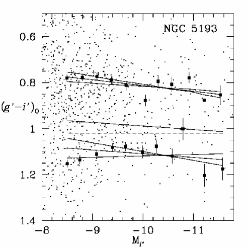
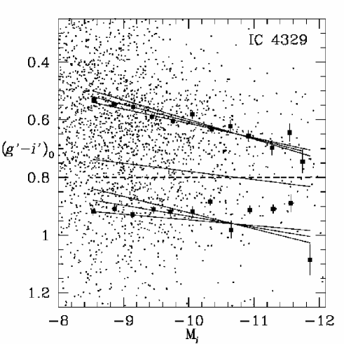
Figure 7: WLSQ fits and their one-sigma errors for the blue and red subpopulations for NGC 5193 and IC 4329. The dashed line shows the initial splitting line and the solid line represents the second splitting line. This solid splitting line results in the blue (red) WLSQ fit and error lines above (below) it.

This red/blue bimodality corresponds to a bimodality in metallicity. Concern has been raised that the split occurs because of a non-linear colour-metallicity relation (e.g., Worthey 1994; Yoon et al. 2006); however, more direct metallicity measurements, including IR colours (Kundu & Zepf, 2007) and spectroscopy (Beasley et al., 2006; Strader et al., 2007; Beasley et al., 2008), argue against this. In addition, the GCS for the Milky Way is found to have a linear (B-I)-metallicity relation (Figure 7 in Harris et al. 2006). M31 also shows bimodality in (U-V)₀, (U-R)₀ and (V-K)₀ colours and metallicity, through spectroscopic and photometric studies presented in Barmby et al. (2000). Bimodality for M31 is not seen in other colours, including (V-I)₀ - a colour often used previously with the testing of bimodality. Barmby et al. suggest, however, that photometric and reddening estimate errors blur away the expected bimodality distribution in these colours (that are actually less sensitive to metallicity).

Another concern is that age and metallicity are degenerate. One attempt to understand this issue was undertaken by Puzia et al. (2005) who used Lick indices to look at the GCSs of seven early-type galaxies. They found that there are three age groups into which GCs fall: two-thirds have an age $>$10 Gyr, one-third are between 5 and 10 Gyrs old, and a small fraction have an age $<$5 Gyrs. The issue of age-metallicity degeneracy remains to be resolved, but the spectroscopic data provide clear evidence that colour bimodality transforms to metallicity bimodality. If age alone could account for the GCS bimodality, a difference of $\Delta(B-I)\approx$ 0.3 would correspond to age differences of 4.5 Gyr and 7.5 Gyr for constant metallicities of [Fe/H]=-2.25 and -1.5, respectively, with the redder clusters being the older subpopulation (Maraston, 2005).

Remaining challenges to unravel are the presence of the two distinct subpopulations and what these may mean for galaxy formation theories. The ideas can be grouped into three main categories: Ashman & Zepf (1992) suggest gas-rich galaxy merging, where each progenitor galaxy has its own blue, metal-poor (MP) GCS and then upon merging the two galaxies create a red, metal-rich (MR) subpopulation. In multi-phase dissipational collapse (Forbes et al., 1997) the GC formation process is halted, for example, via cosmic reionization after a galaxy forms its MP GCs (Beasley et al., 2002; Santos, 2003) and then resumes some time later to form MR GCs. Finally, Côté et al. (1998) suggest that an initially large galaxy has its own MR GCs and then accretes MP GCs from satellite galaxies. Harris (2003) comments that these processes are not mutually exclusive, and are likely to act in a number of combinations for different circumstances.

In addition to the bimodality, a correlation between luminosity and mean colour – that is, a mass-metallicity relation (MMR) – is seen for the blue subpopulation in at least some massive galaxies (e.g., Harris et al. 2006; Mieske et al. 2006; Spitler et al. 2006; Strader et al. 2006). This feature is also referred to as the “blue tilt”. Drawing material from the previously published literature, we list values in Table 1 of the measured MMR slope along the blue GC sequence; this value, $p$, is the exponent in the scaling of heavy-element abundance $Z$ with GC mass $M$, Z$\backsim$M^p. We will discuss the derivation of these slopes and their comparisons in Sections 3 and 4. Columns in Table 1 contain 1) the galaxy sample from which the blue-MMR value was obtained; 2) the value of $p$ for the blue-MMR with errors where available; 3) the brightest GC luminosity values that were used to make the fit, and 4) the reference to the data source paper.

No obvious MMR along the red sequence has been observed (Harris et al., 2006; Mieske et al., 2006; Spitler et al., 2006; Wehner et al., 2008). However, Wehner et al. (2008) detected the red sequence continuing to brighter magnitudes towards the ultra-compact dwarf (UCD) galaxy range. In addition, Strader et al. (2006) interestingly find no blue-MMR in M49 (NGC 4472). If confirmed, this result will provide an additional complexity to be explained by galaxy and globular cluster formation models. Mieske et al. (2006) suggest that environmental causes may produce this result because M49 is at the centre of its own sub-cluster within the Virgo Cluster. This may be an example, they claim, of the differences amongst galaxies with different accretion/merger histories if MMRs are created through GC accretion from galaxies with different masses. Testing this hypothesis, they find that in general GC accretion is unlikely to account for the entire slope of observed MMRs, although it may contribute to or, in the case of M49, negate the trend.

A few other galaxies with smaller GC populations have also been searched for an MMR. Both red and blue slopes for the GC sequences in NGC 1533 are consistent with zero (DeGraaff et al., 2007). This SB0 galaxy is neither in a cluster nor is it a bright elliptical, which the authors imply would be the necessary conditions to produce the self-enrichment that they suggest causes the blue-MMR. The Milky Way does not show any evidence for a blue-MMR, but this may be due to small-number statistics - as there are only $\backsim$150 GCs (Harris, 1996) - rather than the fact that it is a spiral galaxy. Spitler et al. (2006) show that blue-MMRs are not limited to ellipticals as they see a blue-MMR in the Sombrero Galaxy (NGC 4594). Spitler et al. 2006 classify this galaxy as an Sa, although they note that Rhode & Zepf (2004) find it to be an S0. As with ellipticals, no MMR is seen for NGC 4594’s red subpopulation. A key point in assessing the presence or absence of a detectable slope has proven to be the total cluster population in the galaxy (e.g., Mieske et al. 2006): if the MMR slope is most noticeable for the high-luminosity end of the GC sequence ($M\gtrsim 10^{6}L_{\odot}$), it will be unambiguously detectable only in galaxies with thousands of clusters where the high$-L$ end is well populated. For most galaxies, and certainly for most spirals and dwarfs, this upper end is thinly populated and the existence of the MMR is likely to be not decidable.

Spitler et al. (2006) claim that the blue-MMR is not due to the addition of a group of another kind of objects at brighter magnitudes (around M_V $\backsim$ -11), but that the relation continues down to fainter magnitudes - at least to the GC luminosity function turnover magnitude of M${}_{V}^{TOM}$ = -7.6 $\pm$ 0.06. By contrast, Harris et al. (2006) in their study of eight giant ellipticals find that the MMR slope is clearly nonzero only for the brightest blue GCs and that the blue sequence is essentially vertical (i.e., no MMR) for $L\lesssim 6\times 10^{5}L_{\odot}$. Mieske et al. (2006) use a sample of several dozen Virgo galaxies, binned into four groups by galaxy luminosity, to find that the lowest-luminosity members (the dwarfs) show little or no MMR; however, these are also the galaxies for which the high-luminosity end of the GC sequence is least well-populated.

Though this is still a new feature of GCS systematics, several model interpretations for the MMR have already been raised. The most likely ones - both observationally and statistically - appear to have organized themselves around the early enrichment history of GCs during their formation, either from their own internal self-enrichment or from their local surrounding host gas clouds. Working within the hierarchical-merging picture of galaxy formation, Harris et al. (2006) suggest that the blue, MP GCs form first while they are still within dwarf-sized and metal-poor host clouds. The more massive ones can enrich further during formation, thus giving rise to an MMR. By contrast, the red-sequence GCs then form later and are slightly more metal-enriched and red because they form in a deeper potential well when the galaxy formation process has been completed. Strader et al. (2006) and Mieske et al. (2006) favor self-enrichment as the cause of the blue MMR. Quantitative models built on these ideas have been developed by Strader & Smith (2008) and Bailin & Harris (2009).

Although rare, Brightest Cluster Galaxies (BCGs) have uniquely large samples of GCSs which make them the best environments for studying MMRs. In this paper we present newly reduced GC photometric data for two BCGs, NGC 5193 and IC 4329. We follow with a new analysis of the HST data for four more BCGs and further combine them with the data from Harris et al. (2006) and Wehner et al. (2008). We view our discussion in total as one more step towards understanding this intriguing new correlation, which promises to uncover additional clues towards GC formation and enrichment history. Other papers by the authors, both on the observational and theoretical side, are in progress which will help develop a more complete synthesis.

Section 2 details the observations and data reduction of these two galaxies, and is where we also obtain the colour-magnitude diagrams (CMDs) and analyse the MMR. We compare our work with other similar studies and discuss the results in Section 3; we summarize our work in Section 4.

2 New Observations and Data Reduction

We first discuss our new observations for the giant galaxies NGC 5193 and IC 4329. Some uncertainty exists about the status of NGC 5193 and the cluster of galaxies of which it is a part. At times it has been associated with Abell 3560 (e.g. Abell et al. 1989). However, its recession velocity and its projected position indicate that it is neither found at the centre of A3560 nor is it associated with that cluster. The redshift of A3560 is $14470\pm 123$ km s^-1 (Willmer et al., 1999), whereas NGC 5193 and its companion (NGC 5193A) are at $3600$ km s^-1 (Vettolani et al., 1990), and thus NGC 5193 and NGC 5193A appear as foreground objects. NGC 5193 and NGC 5193A are located in Abell 3565 (Willmer et al., 1999; Bardelli et al., 2002). Abell 3565, which has a velocity of $3586\pm 45$ km s^-1 (Willmer et al., 1999) and a richness class of 1 (Abell et al., 1989), is a cluster centred on IC 4296, the brightest galaxy in the cluster (Vettolani et al., 1990; Willmer et al., 1999).

IC 4329 is associated with Abell 3574 which is also known as Shapley 1346-30, K27, the IC 4329 group and Centaurus North (Phillipps et al. 1993 and references therein). IC 4329 also has a richness class of 1 (Abell et al., 1989) and a velocity of 4808 $\pm$ 21 km s^-1 (the CMB reference frame; NASA Extragalacitic Database). Abell 3574 is in turn a member of the Hydra-Centaurus Supercluster.

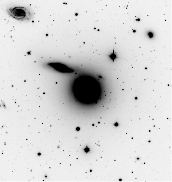
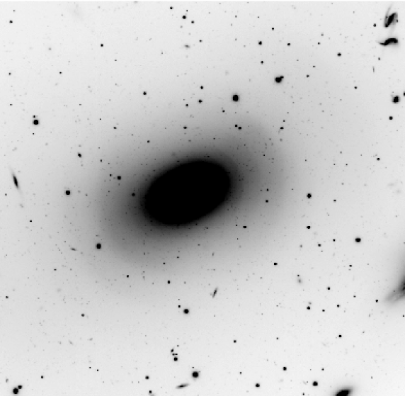
Figure 1: NGC 5193 and IC 4329 Gemini GMOS $g^{\prime}$-band images that have a 5.5’ x 5.5’ field of view and an image scale of 0.146” per pixel, and are from the data set GS-2006A-Q-24.

These two galaxies were observed with the Gemini-South GMOS camera in $(g^{\prime},i^{\prime})$ on the nights of 2006 February 8 and March 23. Images have a 5.5’ x 5.5’ field of view, an image scale of 0.146” per pixel, and come from the data set GS-2006A-Q-24. The two fields can be seen in Figure 1. These images were taken during the same run as NGC 3311, published in Wehner et al. (2008) whose data we re-analyse here to compare with the data from NGC 5193 and IC 4329. Raw exposure times were $13\times 500$ sec in $g^{\prime}$ and $12\times 500$ sec in $i^{\prime}$, similar to the data for NGC 3311. We used the GEMINI/GMOS package within IRAF to preprocess all the images for NGC 5193, IC 4329, and used standard-star exposures taken during the run to calibrate the data. Adopted values of redshift and luminosity are taken from NED. The foreground extinction values were evaluated by using the approximate 1/$\lambda$ relation and the extinctions in the UBVRI system as listed in NED.

NGC 5193 and IC 4329 are at distances of 56.6 $\pm$ 3.8 Mpc and 72.4 $\pm$ 4.6 Mpc (calculated from their values of cz, in the CMB reference frame, as in NED along with H₀ = 70 km s^-1). For a typical GC half-light radius of 3 pc, a GC at a distance of 60 Mpc would subtend an angle of 0.021” which is $\simeq$20 times smaller than the ground seeing FWHM, and so GCs appear entirely star-like. Thus, we can discount the possibility suggested by Kundu (2008) that the blue-MMR is only seen because of aperture-size biasses in high-resolution data.

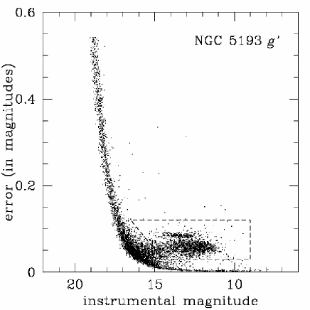
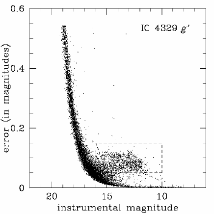
Figure 2: The NGC 5193 $g^{\prime}$-band and IC 4329 $g^{\prime}$-band data sets are shown with plots of instrumental magnitude versus error, and the false identifications within the dashed boxes.

To prepare the images for photometry, we median-subtracted the smoothed isophotal light, allowing the faint star-like objects to be seen more easily in to near the galaxy centres. For the photometry, we used DAOPHOT (the standalone version 4) and ALLSTAR in the same way as described in Wehner et al. (2008). Two of the nine parameters that ALLSTAR returned - the magnitude of the object and the associated error - proved useful to identify false “hits” which were clearly associated with the higher background noise near the brightest regions. These were removed from all later analysis. Examples of these false identifications are shown in the dashed boxes in Figure 2.

We used DAOMATCH to match the detected objects across the $g^{\prime}$- and $i^{\prime}$-band images, with DAOMASTER refining the estimates. Only x- and y-shifts were allowed, leaving coordinate shifts accurate to within $\pm$ 0.1 pixels. Finally, we also used IRAF’s GEOMAP as a consistency check. The final photometry files of matched objects measured in both $(g^{\prime},i^{\prime})$ comprise $1932$ objects for NGC 5193 and $3558$ for IC 4329.

2.1 Calibration

The photometric zeropoints were set from short exposures of standard stars from Landolt (1992), with $(g^{\prime},i^{\prime})$ magnitudes from the catalog by E. Wehner. The GMOS calibration images of these were obtained on the nights of 2006 March 25, 26 and 27, the same nights as the science images. Because only a handful of standard-star exposures were made during the two nights, we view these calibrations as strictly preliminary and note that we intend to improve them in a future paper through a specially designed photometric observing run. Fortunately, as will be seen in the discussion below, our analysis of the MMR and the bimodal sequences depend only on the relative colours, not the absolute scale. The peaks of blue and red subpopulations for many galaxies are virtually constant at a value of $(g^{\prime}-i^{\prime})_{0}\approx$ 0.8 and $(g^{\prime}-i^{\prime})_{0}\approx$ 1.05 (e.g., for M87 with extensive calibration to the SDSS system; Harris 2009). Using this information, we estimate our colour terms to be accurate for NGC 5193, and offset by $(g^{\prime}-i^{\prime})_{0}\approx$ 0.2 for IC 4329 and NGC 3311.

2.2 Colour-Magnitude Diagrams

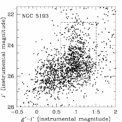
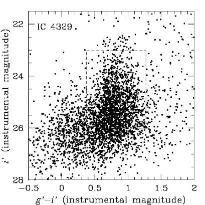
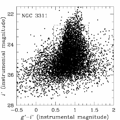
Figure 3: Colour-magnitude diagrams in $(i^{\prime},g^{\prime}-i^{\prime})$ for the two galaxies imaged in our Gemini GMOS program, NGC 5193 and IC 4329, as well as that of NGC 3311 from Wehner et al. (2008) for comparison. GC candidates are located within the dashed-line box. As discussed in Sections 2.2 and 2.3, the brightest limit of the box was incrementally increased in 0.3 magnitude steps.

The colour-magnitude diagrams (CMDs) for the measured objects in both fields are shown in Figure 3, along with the CMD for NGC 3311 (shown for comparison). In these, the GCSs stand out as pairs of vertical sequences. Areas enclosing these vertical sequences were chosen as the areas of interest, to eliminate obvious field contamination. Bright limits were also chosen so that a range of three magnitudes was initially enclosed (while enclosing most of the GCSs, this also allowed the authors to brighten the brightest limits in steps for the later analysis discussed in Section 2.3). Data points were selected from an initial region enclosing the GCS vertical sequences within the limits as follows:

• 0.5 $<$ $(g^{\prime}-i^{\prime})_{0}$ $<$ 1.4 and -11.35 $<$ M${}_{i^{\prime}}$ $<$ -8.35 for NGC 5193,

• 0.25 $<$ $(g^{\prime}-i^{\prime})_{0}$ $<$ 1.25 and -11.4 $<$ M${}_{i^{\prime}}$ $<$ -8.4 for IC 4329 and

• 0.3 $<$ $(g^{\prime}-i^{\prime})_{0}$ $<$ 1.2 and -11.3 $<$ M${}_{i^{\prime}}$ $<$ -8.3 for NGC 3311.

We note that these selection regions are not identical in colour range, but note again that they were chosen with the aim of enclosing the GCS while minimizing field contamination. As also noted above, this is likely to be not because of intrinsic differences between the galaxies, but rather because of remaining errors in the photometric zeropoints as the different galaxies were observed on different nights; but again, the bulk of our later analysis depends only on the relative colours and luminosities. The number of data points within this initial selection region is shown in column (7) of Table 2. We choose to use M${}_{i^{\prime}}$ as the GC luminosity parameter (as opposed to M${}_{g^{\prime}}$) because the values of M${}_{i^{\prime}}$ most closely resemble the bolometric luminosity, and because plotting against the redder colour more accurately portrays the MMR (Mieske et al. 2006; see also our Section 3.1). The faint-end limits of M${}_{i^{\prime}}$$>$-8.35 and -8.4 were estimated visually and adopted to minimize field contamination. The bright-end limits of M${}_{i^{\prime}}$$<$-11.4 and -11.35 were only initial and were later increased in steps (see below) to see what effect, if any, this would have on the deduced MMRs.

In Figure 4, we show the radial distribution of the GC candidates around each galaxy (see Appendix for a more detailed description of these diagrams, including calculation of the GCS specific frequencies). As the CMDs also indicate, the GCS around NGC 5193 is the less populous of the two, and is also the more centrally concentrated with a steeper power-law fit.

The first step in the analysis is to test the colour distribution of the GCs for clear presence (or absence) of bimodality. To do this, we used the multimodal statistical fitting package RMIX in the same way as described more fully in Wehner et al. (2008). We carried out one-, two- and three-Gaussian fits with the sample divided into colour bins of $(g^{\prime}-i^{\prime})$ = 0.045, and for comparison we included the previously published NGC 3311 data as well. A normal chi-squared test shows that two modes are strongly preferred over only one, but three modes produced no further improvement with either the hetero- or homoscedastic fits. A homoscedastic fit forces the dispersions of both subpopulations to be the same, whereas a heteroscedastic fit allows them to be independent. We therefore argue that the two-Gaussian fit is the optimal solution, indicating that these galaxies are basically similar to other giant ellipticals. The RMIX fits are shown in Figure 5 and all parameters for these fits are shown in Table 4. Columns contain (1) the target’s NGC or IC number, (2) the proportion of the subpopulation, (3) the error on the proportion, (4) the mean value of the Gaussian fitted to the subpopulation (i.e., the peak colour value), (5) the error on the mean, (6) the sigma, or distribution value, (7) the error on sigma (not applicable for the second subpopulation because the values of sigma for both subpopulations was forced to be equal), (8) the degrees of freedom in the fit, (9) the $\chi^{2}$ value, and (10) the reduced $\chi^{2}$ value, found by dividing $\chi^{2}$ by the degrees of freedom. We argue the use of homo- versus heteroscedastic fits for several reasons. Significant overlap between the two subpopulations for all three galaxies - NGC 5193, IC 4329 and NGC 3311 - causes the peaks in the distribution to become obscured. Allowing a larger number of free parameters in such a scenario makes an RMIX fit harder to converge. When we allow a heteroscedastic fit to the subpopulations of IC 4329, we find that the sigma values are equal within errors. Wehner et al. (2008) obtain a similar result for NGC 3311. However, for NGC 5193 we find that a heteroscedastic fit has discrepancies of $\sigma(g^{\prime}-i^{\prime})$ = 0.16$\pm$0.01 and 0.10$\pm$0.2 for the blue and red subpopulations, respectively. With heteroscedastic fits, we also find that the proportion of GCs within each subpopulation becomes more unrealistic, especially for NGC 5193: 0.86$\pm$0.06 and 0.14$\pm$0.06 for the blue and red subpopulations in NGC 5193, respectively, 0.61$\pm$0.14 and 0.39$\pm$0.14 in IC 4329, and 0.78$\pm$0.04 and 0.22$\pm$0.04 in NGC 3311. As we were concerned that these above effects were amplified by NGC 5193 GCS’s low numbers, we forced all the fits to be homoscedastic. Even though the reduced chi-squared value for the two-Gaussian fit on the NGC 3311 GCS is the lowest of the different fits tried, we note that it is still unusually high. Various smaller bin sizes were tried in the two-Gaussian fit, but the proportions and peak values of the subpopulations remained the same.

The peak values of the red and blue subpopulations for the three Gemini galaxies (including comparison with NGC 3311) are not the same, again because of residual zeropoint errors as noted above. However, it is important to note that the differences between the colours of the blue and red peaks $\Delta(g^{\prime}-i^{\prime})_{(red-blue)}$, are the same among all three galaxies, indicating that their metallicity differences are similar.

2.3 Analysis of the Mass-Metallicity Relation

Quite simply, a mass-metallicity relation for either the blue or red GC sequences will exist if the mean colour changes systematically with luminosity. The two techniques that have previously been used to find it are either to assume a linear relation between mean colour and absolute magnitude and solve for the slope (Strader et al., 2006; Spitler et al., 2006; DeGraaff et al., 2007; Wehner et al., 2008); or, to bin the data in magnitude steps and find the mean colour of each sequence in each bin (Harris et al., 2006; Mieske et al., 2006; Wehner et al., 2008; Harris et al., 2009). In this paper, we use the former as the main method and compare to the latter.

The data set for each GCS was sorted into 0.3 magnitude bins in $M_{i^{\prime}}$ so that enough bins along the sequence were generated while also maintaining enough GCs per bin to be statistically significant. Then to reduce field-star contamination further, we applied an approximate representation of the Chauvenet criterion (Parratt, 1961) to each bin. The criterion’s purpose is to reduce the biasing effect of outlying points on values for the mean and standard deviation. We found the mean colour and its uncertainty $\sigma_{mean}$, for each bin and discarded outlying points if their colours fell farther from the bin mean than z$\sigma_{mean}$ , where

$$z\simeq 0.85(log_{10}n)+1.12$$ (1)

and n is the number of points in the bin.

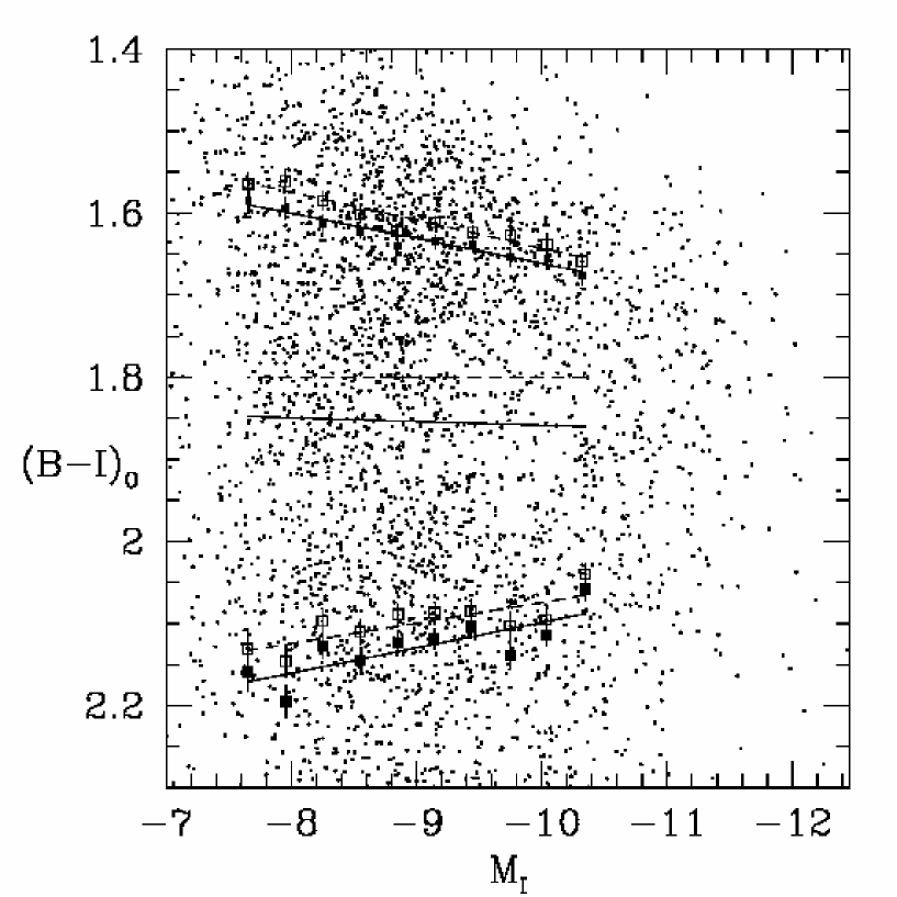
Figure 6: A CMD for NGC 4696, with an example of initial constant dividing line with a value of (B-I)₀=1.8 (the middle dashed line) and then a subsequent sloping dividing line (the middle solid line). The sloping dividing line is placed exactly half-way between the initial WLSQ fits (the upper and lower dashed lines). See Section 2.3.

To get colour-magnitude slopes (i.e., $\Delta(g^{\prime}-i^{\prime})/\Delta M_{i^{\prime}}$), we first split the data points into red and blue sides with a line at one colour value, although the value of this initial dividing line varies from GCS to GCS as discussed below. Figure 6 shows the published data in NGC 4696, which we use as an example for illustrative purposes. The middle dashed line in this figure represents the initial dividing line. The value of the initial dividing line for each GCS is chosen to be at the “dip” colour value (Peng et al. 2006b, 2008; i.e., the colour where a GC has equal probability of being red or blue). Peng et al. (2008) note that although the mean colours of subpopulations may vary with galaxy luminosity, the dip colour is nearly the same. As our data sets have yet to be well-calibrated we can see that our dip colours are not all the same: IC 4329 and NGC 3311 have very similar dip colours of (g-i)₀=0.78 and 0.80, respectively, whereas NGC 5193’s dip colour is (g-i)₀=1.02. However, knowing that the dip colour values should be constant, we choose the dip colour of the GCS as the initial dividing line. We then binned the two data subsets in 0.3 magnitude bins, finding a mean for each bin. Finally, we calculated a weighted least-squares (WLSQ) linear fit of bin magnitude versus bin colour for each subset (the upper and lower dashed lines in Figure 6).

A line (the middle solid line in Figure 6) exactly half-way between these two initial fits was used to split the Chauvenet-excluded data set a second time, and the process was repeated. This second splitting was to compensate for any inequality in the proportions of the two subpopulations (see Section 3.2). The upper and lower solid lines in Figure 6 show the final WLSQ fits. Figure 7 shows the CMDs and MMRs for NGC 5193 and IC 4329 (with only 11 and 12 bins, respectively), where we also added the one-sigma error bars of the WLSQ fit to the adopted linear solutions. If we were to eliminate the brightest bin in the red slope of IC 4329, we can see that within errors the fitted slope would immediately drop to zero. This outlying bin is excluded on similar grounds to the Chauvenet criteria, as was a similarly outlying point excluded in NGC 5322.

As noted above, the upper, brighter limit of the selection region was incrementally increased in 0.3 magnitude steps to explore what effect - if any - it had on the colour-magnitude slope. We used three methods to do this. For each subpopulation in each GCS in our first method, we started with a minimum of ten bins for which we calculated a slope. Bins at brighter magnitudes were added until there were no more GCs to bin. With each new bin added a new slope was calculated. This gave us up to five slopes per subpopulation per GCS. NGC 5193 had so few points that only the slopes for 10 bins and 11 bins could be measured (i.e., only one bin was added to the bright end). The two blue $\Delta(B-I)_{0}/\Delta M_{I}$ slopes were the same within errors (-0.05$\pm$0.03 and -0.05$\pm$0.02), as were the red (-0.01$\pm$0.05 and -0.03$\pm$0.04). For IC 4329, slopes for 10-13 bins were calculated (i.e., three bins were successively added to the bright end). The IC 4329 blue slopes varied between $\Delta(B-I)_{0}/\Delta M_{I}$=-0.11$\pm$0.02 and -0.05$\pm$0.01, and we found that the red varied between $\Delta(B-I)_{0}/\Delta M_{I}$=-0.07$\pm$0.03 and 0.05$\pm$0.02. The values of all blue and red slopes are shown in Table 3. The IC 4329 slopes for 12 and 13 bins are shown with and without the outlying point.

The second method used a constant number of ten bins. As a brighter bin was added, the faintest bin was dropped and a new slope was calculated. Again, this gave up to five slopes per subpopulation per GCS. To look at any possible curvature of the MMR we used the IRAF/POLYFIT routine for our third and final method with a polynomial of order two. We input both the minimum number of ten bins, and also the maximum number of up to fourteen bins in the routine and compared the results.

With the first two methods, we saw no consistent change on the MMR slopes as brighter bins were included. With the final method, most slopes had an insignificant second-order component. The remaining few only had a marginal second-order component. We conclude that a linear slope for the MMR is a reasonable assumption for our sample of galaxies, and that the particular choice of bins (luminosity range) has no major effects on the deduced slope.

To compare all slopes, we used the slope with the maximum number of bins, but excluding the faintest and brightest bins. This was done to reduce the effects of field contamination (at the faint end) and small numbers (at the bright end).

3 Comparison and Discussion

Part of the purpose of our study is to search further for any trends in the slope of the MMR with such factors as host galaxy luminosity or environment. To our MMR solutions for NGC 5193 and IC 4329, we now add similar results from other BCGs or giant ellipticals. Previously published ones include the eight in Harris et al. (2006) and NGC 3311 in Wehner et al. (2008). To these, we add a further four BCGs - NGCs 7626, 708 and 7014, and IC 4296 (Harris et al., 2009) - observed with HST in $(B,I)$, similar to those in Harris et al. (2006). For the total of 15 BCGs listed above, Table 2 lists in successive columns (1) the target’s NGC or IC number, (2) the galaxy group or cluster, (3) the redshift cz of the galaxy, (4) the galaxy luminosity, M${}_{V}^{T}$, (5) the foreground reddening, (6) the apparent distance modulus (either SBF-based distances from Tonry et al. (2001) were used, as is the case for the galaxies marked with (i), or these values were calculated from radial velocities using an adopted value of H₀ = km s^-1 Mpc^-1), (7) the number of data points within the initial selection region (see Section 2.2 for details of the selection regions), (8) the total number of GCs estimated to be in the system, and (9) the specific frequency, S_N.

Mieske et al. (2006) conducted an MMR study for 79 early-type galaxies with HST/ACS photometry in $(g_{475}-z_{850})$ as part of the Virgo Cluster Survey. Though most of these galaxies are dwarfs or ones with small globular cluster populations in which no individual MMR solutions can be determined, they combined their sample into four bins grouped by galaxy luminosity. In each bin the total GC sample is then large enough for any cumulative MMR slope to be found with some confidence. These four bins are compared with the BCG data sets.

3.1 Comparisons to Other Data

To put all these studies onto a common system for comparison requires converting three different colour indices: $(g_{475}-z_{850})$, $(B-I)$, and $(g^{\prime}-i^{\prime})$. In each case we convert $\Delta(colour)/\Delta(mag)$ into a scaling exponent $p=\Delta\rm{log}Z/\Delta\rm{log}M$. There is currently no established relation between $(g^{\prime}-i^{\prime})$ and metallicity for GCs, so we first converted $(g^{\prime}-i^{\prime})$ to $(B-I)$, although we note that this double conversion introduces larger external uncertainties. With single stellar population models from Maraston (2005) we calculated the linear colour conversion:

$$\Delta(B-I)=\frac{\Delta(g^{\prime}-i^{\prime})}{(0.53\pm 0.12)}.$$ (2)

To convert to metallicity from (B-I) colours, we used the linear relation as in Harris et al. (2006), which is based on colours and metallicities for Galactic GCs:

$$\frac{\Delta(B-I)_{0}}{\Delta[\textrm{Fe/H}]}=0.375\pm 0.049$$ (3)

Mieske et al. (2006) obtain their $(g_{475}-z_{850})$ colour-metallicity conversion from Peng et al. (2006b), who have a piecewise relation that is based not only on Galactic GCs but also GCs in M87 and NGC 4472:

$$\frac{\Delta(g_{475}-z_{850})}{\Delta[\textrm{Fe/H}]}=0.195\pm 0.025\hskip 28.45274pt[0.70<(g_{475}-z_{850})\leqslant 1.05]$$ (4)

$$\frac{\Delta(g_{475}-z_{850})}{\Delta[\textrm{Fe/H}]}=0.546\pm 0.069\hskip 28.45274pt[1.05<(g_{475}-z_{850})<1.45]$$ (5)

We note that Peng et al. (2006b) actually mean log Z rather than [Fe/H]. These two quantities are different by a factor of [$\alpha$/Fe], which we assume to be constant so that the $slope$ remains the same when converting between colour and metallicity.

The compilation of results for this entire extended sample of galaxies is shown in Figure 8, as a graph of scaling slope $p$ against host galaxy luminosity. Here, we show the MMR for each galaxy for both the blue and the red subpopulations. For the Mieske et al. (2006) data, each galaxy has two data points plotted. The data set represented by open triangles is $(g_{475}-z_{850})$ versus $g_{475}$-magnitude, while the data set represented by solid triangles is $(g_{475}-z_{850})$ versus $z_{850}$-magnitude. Mieske et al. argue that the $(M_{z_{850}},(g_{475}-z_{850}))$ relation is to be preferred, because cross-contamination biasses between the two modes affect the $(M_{g_{475}},(g_{475}-z_{850}))$ relation more strongly. We consider only the $(M_{z_{850}},(g_{475}-z_{850}))$ data points (solid triangles) in our discussion.

For galaxies brighter than $M_{V}^{T}\simeq-19$, we find that the blue slopes have a mean $p-$value of $p=0.30\pm 0.05$. For the red slopes, we find $p=-0.1\pm 0.1$, which is consistent with zero. $P$-values of blue and red slopes are shown in Figure 8. The dwarf galaxies in the faintest bin of Mieske et al. (2006) have $p=0.11\pm 0.18$ for the blue-MMR. However, we note that this lower value may be because there are fewer high-luminosity GCs in that bin - even after adding all the dwarfs together. Therefore, if the MMR is more prominent at higher parent galaxy luminosities, it would affect the dwarf/giant comparison. We find a consistent $p-$value roughly independent of the individual GC luminosity range, although at increasingly fainter levels down along the GC sequences the determination becomes less certain because of increasing photometric scatter and field contamination.

Note that our error of $\Delta p$=0.05 is an $internal$ error on the slope and does not include the transformation errors from $(B-I)_{0}$ to metallicity or from $(g^{\prime}-i^{\prime})$ to metallicity, which are approximately $\Delta p\approx$0.02 and 0.2, respectively. These additional $external$ uncertainties are the inevitable result of combining different photometric systems, but as far as we can determine, they do not affect our overall conclusion that $p\approx$ constant for the more luminous galaxies. Further, more strictly homogeneous surveys would remove this lingering uncertainty.

3.2 Comparing Different Methods

We now test whether or not the line splitting method we used above may have actually introduced the observed MMR. Suppose we have a situation where the mean colours of both red and blue modes stay constant with luminosity, but where the numbers of GCs in the two modes might be different. Suppose also (realistically) that the random measurement uncertainties increase with magnitude, so that the two modes would overlap more and more as we go to fainter magnitudes. If the two subpopulations contained equal numbers of GCs, MMRs would not be seen (i.e., they would be consistent with zero) because similar numbers of clusters in each mode would contaminate the other mode. However, if the blue subpopulation dominated, and the same constant dividing line was used, a positive offset for both subpopulations would be seen: more blue clusters would spill into the red side than vice versa, so the measured mean colour of both modes would be too blue at the faint end of the sample. In this case, we would conclude that the mean colours of both modes became redder at brighter magnitudes. Conversely, if the red subpopulation dominated, a negative offset for both subpopulations would be seen. For this reason, we used the second iteration of the line splitting to counter this effect.

We do not see this contamination-based effect happening in any of the solutions for our sample galaxies. For the blue mode, the $p-$values are consistently positive, whereas for the red mode the slopes are slightly negative and consistent with zero. In particular, for the red-dominated GCSs (NGCs 1407, 5322, 7049, 3348, 4696ap, 5557 and 7626, and IC 4296) the red-mode slopes are all slightly negative or close to zero, which is consistent with the above argument. However, in these same GCSs the blue-mode MMRs have an average value around p $\backsim$ 0.30, which is not consistent with the argument and therefore provides some support for the analysis method.

Another and different factor, which we cannot assess as completely here, is the amount of field contamination. Although we selected restricted intervals in colour to minimize the contamination, it is notably worse at fainter magnitudes and if the contamination is asymmetric in colour, it could bias the RMIX fits. An argument against such an effect, however, is that the Mieske et al. (2006) Virgo sample is contamination-free (the GCs were identified individually) and their mean results are no different from ours at the same galaxy luminosities. In addition, the different galaxies in our sample have different degrees of field contamination (cf. the individual source papers) but yield very similar MMR slopes.

We have also compared our results with methods using the KMM bimodal fitting code, including six galaxies from Harris et al. (2006), and for the three Gemini/GMOS galaxies by conducting RMIX fits. (Only six of the eight Harris et al. galaxies are used because two galaxies only have one bin per subpopulation; each bin contains 200 points.) The Gemini data sets were divided into 0.5 magnitude bins, with the brightest two bins in NGC 5193 and IC 4329 not being included in the fit because of the very low numbers of GCs there. Comparisons were made between RMIX and KMM, as shown in Table 5 and Figure 10. Six of the nine blue-MMRs and a different six of the nine red-MMRs are consistent within errors for both methods, further supporting the line splitting method and showing that the codes are consistent.

We find a blue-MMR index at a constant value of 0.30$\pm$0.05. However, two galaxies are clearly outside that range: NGC 3311, which has a much higher index, and IC 4296 which has an index that within the errors is consistent with zero. We also recall that M49 (NGC 4472), included in the brightest bin of the Mieske et al. (2006) data set, also does not show a blue-MMR.

3.3 No Correlation with Specific Frequency

The fifteen GCSs in Table 2 can be split into two groups: sparse GCSs, which we define in a similar manner to Harris et al. (2006) to have specific frequency, S_N$\leq$5; these include NGCs 1407, 5322, 3348, 3268, 5557, 7626 and 5193, and ICs 4296 and 4329; and rich GCSs, defined to have S_N$>$5; these include NGCs 7049, 3258, 4696, 708, 7014 and 3311 (see the Appendix in Section 5 for $S_{N}$ calculations). We find no significant difference in the average MMR slope ($p-$value) between these two groups (see Figure 9), although we note that NGC 3311 is a significant outlier. The lack of correlation of $p$ with $S_{N}$ is consistent with the interpretation that the source of the MMR is one more local to the GCs themselves (such as self-enrichment) rather than one driven by the large-scale GC formation efficiency.

4 Summary

We discuss the photometry for globular cluster systems in fifteen BCGs and use these to derive the MMRs for both the red and blue globular cluster subpopulations. Twelve data sets were from the HST, and a further three data sets were obtained from Gemini/GMOS with $(g^{\prime},i^{\prime})$ photometry. The eight ACS/WFC data sets and one Gemini data set were previously analysed in Harris et al. (2006) and Wehner et al. (2008), respectively. For the other two GMOS datasets (NGC 5193 and IC 4329) we present the photometry and its results for the first time.

Colour-magnitude slopes were found via a “line splitting” method, and converted to an MMR in heavy-element abundance versus mass ($Z\sim M^{p}$) so that comparisons between the HST and Gemini data, and with the Virgo Cluster Survey galaxy sample (Mieske et al., 2006) data, could be made. We use the composite results to construct a plot of the scaling exponents - $p(blue)$ and $p(red)$ - versus host galaxy luminosity and also versus specific frequency.

Our work confirms the existence of a blue-MMR with Z$\backsim$M^0.30±0.05, independent of host galaxy luminosity for any systems brighter than $M_{V}^{T}\simeq-19$. Individual galaxy-to-galaxy differences may still exist (with occasional anomalies such as NGC 4472, whose lack of an MMR still remains to be explained) but are still hard to determine unambiguously. For the dwarf galaxies fainter than $M_{V}^{T}\sim-19$, the blue-MMR slope is consistent with zero, though we raise the question that this might be due to the smaller number of GCs at high luminosities, making the MMR less noticeable. Whether or not the MMR continues to lower GC luminosities with the same slope remains an open question, because of the increasing effects of field contamination and photometric measurement scatter.

Within the measurement uncertainties, the red-sequence MMR is consistent with a line that includes zero (Z $\backsim$ M^-0.1±0.1). We also find no correlation between the $p$-values of slopes and specific frequencies.

We have tested our line splitting method numerically to confirm that that nature of the method does not itself artificially introduce an MMR. In general we find clear agreement between the line splitting method and multimodal histogram fitting methods employing RMIX and KMM.

The results of this paper agree partially but not completely with Mieske et al. (2006), who show that for lower host-galaxy luminosities, i.e., dwarf galaxies, the blue-MMR is not the same as those for mid-range host-galaxy luminosities. Here, we add many more galaxies to the brightest range and find similar relations to those of the mid-range. We note that NGCs 3311 and 4296 lie offset from the rest of the galaxies for the blue-MMR in Figure 8. Only the dwarf ellipticals stand out as having no clear MMR amongst their globular clusters. This suggests that similar GC formation processes occurred in BCGs as occurred in typical early-type galaxies.

The clear existence of a blue-sequence MMR is, in general, consistent with recent models in which the higher mean metallicities within more massive GCs are due to self-enrichment within the proto-GC: they form in more massive potential wells which can hold in a higher fraction of supernova-driven enrichment (e.g., Bailin & Harris 2009). Within the same interpretive framework, the lack of a similar trend along the red GC sequence is expected if their mean metallicity is due to a higher level of pre-enrichment, above which any later self-enrichment would be less important. The independence of $p$-values versus both host galaxy luminosity and specific frequency may favour interpretations where the MMR is due to local events in and near where the clusters form, rather than the global environment of the galaxy itself.

We suggest follow-up observations for galaxies as a function of environment, especially isolated giant elliptical galaxies. Also, it is statistically difficult to see any MMRs in spiral galaxies, but if they could be stacked together in a similar manner to the dwarf galaxies in Mieske et al. (2006) then perhaps a trend would become apparent.

5 Appendix

To estimate the total number of GCs in the Gemini systems, we first counted the number of GCs within similar limits of Section 2.2:

• 0.5 $<$ $(g^{\prime}-i^{\prime})_{0}$ $<$ 1.4 and M${}_{i^{\prime}}$ $<$ -8.35 for NGC 5193 and

• 0.25 $<$ $(g^{\prime}-i^{\prime})_{0}$ $<$ 1.25 and M${}_{i^{\prime}}$ $<$ -8.4 for IC 4329.

These magnitudes were converted to M_V with the ugriz standard star catalogue by E. Wehner referenced in Section 2.1. (i’-V) was plotted against (g’-i’) and the following conversion equation was obtained:

$$(i^{\prime}-V)=-0.69(g^{\prime}-i^{\prime})+0.8238$$ (6)

The radial distribution of the objects falling in these magnitude and colour ranges, relative to the centre of each galaxy, is shown in Figure 4. Here the number density (objects per unit area) is plotted against galactocentric distance in linear form, extending out to the edges of the GMOS frame. The outer regions of the NGC 5193 field were used to set an approximate background level for both fields and this was subtracted from the counts before plotting. Then, to estimate the total GC population within the field, we fit a simple power law of the form $\sigma=\beta r^{-\alpha}$ and integrated out to the edge of the image. The power laws, after being amplitude adjusted, were $\sigma=313.2\pm 50.4r^{-2.66\pm 0.22}$ and $\sigma=7.12\pm 1.52r^{-1.34\pm 0.10}$ for NGC 5193 and IC 4329, respectively. As this estimate does not cover the entire radial extent of the GCS, we corrected for the field of view in our images.

We then assumed that for a gE the number of GCs per unit magnitude is described by a Gaussian with a mean value of M_V = -7.33 and a standard deviation of 1.4 magnitudes (Harris, 2001). This allowed us to find the fraction of GCs brighter than the limiting magnitude. By dividing the number of GCs above the limiting magnitude by this fraction, the estimate for the total number of GCs in the system was finally obtained (i.e., the values in column (8) in Table 2). The specific frequency, S_N is then calculated from

$$S_{N}=N_{GC}10^{0.4(M_{V}+15)}$$ (7)

(Harris & van den Bergh, 1981). For the remaining galaxies, we either adopted values of $S_{N}$ from the literature or, if there were no previous values, we calculated $S_{N}$ in a method similar to the above without the FOV correction. For $HST$ data, limiting magnitudes were converted to M_V with UBVRI standard star data from Landolt (1992). (V-I) was plotted against (B-I) and the following conversion equation was obtained:

$$(V-I)=0.53(B-I).$$ (8)

Table 1: Summary of MMRs in Previously Observed Galaxies

Galaxy sample	$p$	Brightest GC Luminositya	Reference
(1)	(2)	(3)	(4)
8 BCGs	0.55	MI$>$-13.0	Harris et al. (2006)
NGC 3311	0.6	MI$>$-13.5	Wehner et al. (2008)
Virgo galaxiesb	0.48$\pm$0.08	MZ$>$-12.0	Mieske et al. (2006)
M87	0.48	MZ$>$-12.2	Strader et al. (2006)
NGC 4649	0.43	MZ$>$-12.0	Strader et al. (2006)
NGC 4472 (M49)	0	MZ$>$-11.8	Strader et al. (2006)
NGC 5866	0.11$\pm$0.09c	MR$>$-10.2	Cantiello et al. (2007)
NGC 1533	0	MI(814)$>$-10.2	DeGraaff et al. (2007)
NGC 4594 (Sombrero Galaxy)	0.27	MR$>$-11.6	Spitler et al. (2006)
a Values of cz and extinction from NED were used with an adopted value of
H0 = 70 km s-1 Mpc-1 to calculate absolute magnitudes for M87, NGC 4649, NGC 4472,
NGC 5866, NGC 1533 and NGC 4594.
b Mieske et al. (2006) study 79 early type galaxies which they split into four host-galaxy
magnitude bins. The MMR cited above is for their brightest bin where the host-galaxy magnitude
range is -21.7$<$MB$<$-21.
c Cantiello et al. (2007) caution that this result is tentative because of the small number of
GCs (109) used to find these slopes.

Table 2: Data for Individual BCG Galaxies

NGC or IC	Cluster or Group	Redshift cz	M${}_{V}^{T}$	E(B-I)	(m-M)I	Number of	NGC	SN
		(km s-1)				data points
(1)	(2)	(3)	(4)	(5)a	(6)b	(7)c	(8)	(9)
(B, I) photometry from ACS/WFC
NGC 1407	Eridanus	1627i	-22.4	0.16	32.0	1046	2641$\pm$303d	4.0$\pm$1.3d
NGC 5322	CfA 122	1916i	-22.0	0.03	32.2	395	1600	2.5
NGC 7049	N7049	1977i	-21.8	0.12	32.4	682	2700	5.8
NGC 3348	CfA 69	2902a	-22.2	0.17	33.2	831	3100	4.4
NGC 3258	Antlia	3129i	-22.1	0.20	33.4	1812	6000$\pm$150e	6$\pm$2.5e
NGC 3268	Antlia	3084i	-22.1	0.24	33.4	1593	4750$\pm$150e	3$\pm$2e
NGC 4696	Cen 30	3248i	-23.0	0.23	33.5	3099	4100$\pm$200f	6f
NGC 5557	CfA 141	3389a	-22.4	0.01	33.4	841	3500	4.1
NGC 7626	Pegasus (I)	3154j	-22.4	0.17	33.4	1835	2833$\pm$300g	3.9g
B photometry from ACS/WFC, I from WFPC2
NGC 708	Abell 262	4601a	-22.1	0.21	34.3	1282	4800	7.2
NGC 7014	Abell 3742	4676a	-21.8	0.08	34.2	962	3800	7.4
IC 4296	Abell 3565	4009a	-23.4	0.15	33.8	885	36000	1.7
(g, i) photometry from GMOS
NGC 5193	Abell 3565	3988a	-22.4	0.11	33.9	596	630$\pm$330	0.70$\pm$0.36
IC 4329	Abell 3574	4808a	-23.1	0.12	34.3	1528	2970$\pm$530	1.56$\pm$0.28
NGC 3311	Abell 1060	3937a	-22.4	0.15	34.0	4936	16500$\pm$2000h	12.5$\pm$1.5h
a Values were taken from NED.
b Values calculated using an adopted value of H0 = 70 km s-1 Mpc-1.
c Points in the initial selection regions as detailed in Section 2.2
Values from
d Perrett et al. (1997).
e Bassino et al. (2008).
f Lee & Geisler (1999).
g Sikkema et al. (2006).
h Wehner et al. (2008).
i Tonry et al. (2001).
j Ramella et al. (2002).

Table 3: Blue and red $\Delta$(B-I)₀/$\Delta$M_I slopes with corresponding p values for all bins, where p is defined in the relation Z = M^p. Errors are shown as the internal relative error of the original slopes (i.e., errors due to the colour transformation are not propagated). The IC 4329 slopes for 12 and 13 bins are shown with and without the outlying point mentioned in Section 2.3.

NGC	Number	Blue	Blue Slope	p	Error	Red	Red Slope	p	Error
or IC	of bins	Slopea	Errora		on p	Slopea	Errora		on p
(1)	(2)	(3)	(4)	(5)	(6)	(7)	(8)	(9)	(10)
NGC 5193	10	-0.05	0.03	0.31	0.56	-0.01	0.05	0.05	0.78
NGC 5193	11	-0.05	0.02	0.32	0.45	-0.03	0.04	0.21	0.77
IC 4329	10	-0.08	0.01	0.51	0.32	0.02	0.02	-0.14	0.44
IC 4329	11	-0.05	0.01	0.35	0.33	0.05	0.02	-0.33	0.44
IC 4329(-outlier)	12	-0.11(-0.111)	0.02(0.003)	0.74(0.74)	0.53(0.30)	-0.07(0.01)	0.03(0.02)	0.48(-0.04)	0.73(0.36)
IC 4329(-outlier)	13	-0.08(-0.082)	0.01(0.003)	0.55(0.55)	0.42(0.23)	-0.06(0.01)	0.03(0.02)	0.42(-0.06)	0.64(0.38)
NGC 3311	10	-0.106	0.003	0.71	0.28	0.006	0.005	-0.038	0.090
NGC 3311	11	-0.103	0.003	0.69	0.27	0.007	0.004	-0.050	0.080
NGC 3311	12	-0.118	0.006	0.79	0.36	0.005	0.003	-0.033	0.059
a Values converted from (g-i)0 to (B-I)0

Table 4: RMIX Multimodal Fitting Parameters for Gemini/GMOS Galaxies

Target	Pi	Error	Mean	Error	Sigma	Error	DOF	$\chi^{2}$	Reduced	pr($>\chi^{2}$)
									$\chi^{2}$
(1)	(2)	(3)	(4)	(5)	(6)	(7)	(8)	(9)	(10)	(11)
NGC 5193	0.70	0.05	0.81	0.01	0.144	0.007	19	46.1	2.4	2.2x10-16
	0.30	0.05	1.11	0.02	0.144	NA
IC 4329	0.68	0.03	0.592	0.009	0.150	0.005	18	69.8	3.9	4.8-4
	0.32	0.03	0.90	0.01	0.150	NA
NGC 3311	0.57	0.02	0.610	0.005	0.142	0.003	19	221	11.6	4.8x10-8
	0.43	0.02	0.898	0.006	0.142	NA

Table 5: Comparison of Line Split $\Delta(B-I)_{0}/\Delta M_{I}$ Slopes For Blue and Red GC Sequences. Pairs that do not agree within the errors are highlighted in bold. The slopes for the line split bins are from the WLSQ fits that have the maximum number of bins minus the faintest and brightest bins.

Galaxy	Method	Blue	Error	Red	Error
		Slope		Slope
(1)	(2)	(3)	(4)	(5)	(6)
NGC 1407	Line split bins	-0.041	0.011	0.0168	0.0077
	KMM peaks	0.00	0.03	0.03	0.03
NGC 3348	Line split bins	-0.0517	0.0081	0.0148	0.0065
	KMM peaks	-0.04	0.02	0.027	0.008
NGC 3258	Line split bins	-0.0495	0.0027	0.0083	0.0064
	KMM peaks	-0.04	0.01	0.00	0.01
NGC 3268	Line split bins	-0.0571	0.0030	0.0113	0.0075
	KMM peaks	-0.061	0.005	-0.01	0.01
NGC 4696	Line split bins	-0.0314	0.0040	0.0486	0.070
(aperture)	KMM peaks	-0.04	0.01	-0.04	0.02
NGC 5557	Line split bins	-0.0498	0.0054	-0.0035	0.0077
	KMM peaks	-0.030	0.003	-0.015	0.007
NGC 5193a	Line split bins	-0.025	0.018	-0.012	0.032
	RMIX peaks	-0.11	0.03	0.03	0.09
IC 4329a	Line split bins	-0.0400	0.0089	-0.033	0.021
	RMIX peaks	-0.03	0.01	0.03	0.01
NGC 3311a	Line split bins	-0.0545	0.0012	0.0038	0.0023
	RMIX peaks	-0.060	0.005	-0.012	0.007
a Values remain in $(g^{\prime}-i^{\prime})_{0}/M_{i^{\prime}}$

Figure 4: Number of GC candidates per unit area on the sky as a function of projected galactocentric radius, after background subtraction. The radial bins used were 50 pixels wide, corresponding to 7.3 arcseconds. NGC 5193 and IC 4329 have scales of 3.64 and 2.85 arcseconds/kpc, respectively. The error bars equal ($n^{0.5}$/area) for $n$ candidates in each bin. The upper horizontal dashed line in each panel shows the adopted background level $\sigma_{b}$, chosen from the outer regions of the NGC 5193 field where the observed number density is nearly level. The power-law fits described in the Appendix were determined from the data points within the two vertical dashed lines: the inner one represents the point within which the detections of the GC candidates become hampered by the increasing light of the central bulge, whereas the outer line represents the largest radius at which a complete annulus fits inside the GMOS field.

Figure 5: The two-Gaussian solutions for the RMIX fits of NGC 5193 and IC 4329 data sets. The parameters of these fits are shown in Table 4. We note that although the distributions look like they could be fit with a skewed unimodal solution, we assume bimodality from previous studies (e.g., Harris et al. 2006; Mieske et al. 2006; Spitler et al. 2006; Strader et al. 2006).

Figure 8: Mean of blue and red MMR indices plotted against host-galaxy luminosity. For our data sets (filled circles), the one-sigma errors that were calculated for the colour-magnitude slopes are shown as the same relative error on $p$ here. Transformation errors are not included here but are approximately $\Delta p\approx$0.02 and 0.2 for $(B-I)_{0}$ to metallicity transformations and $(g^{\prime}-i^{\prime})$ to metallicity transformations, respectively. The data points of Mieske et al. (2006) are shown here for comparison; ($g-z,z$) and ($g-z,g$) as filled and open triangles, respectively. The errors for their points come from a random resampling around the KMM fits (see their Table 1). Note that although we tested 15 GCSs, there are actually 16 points plotted above. The two data points at $M^{T}_{V}$=-23 are both for NGC 4696, with the upper (lower) data point corresponding to the method using PSF (aperture) photometry (Harris et al., 2006).

Figure 9: Mean of blue and red MMR indices plotted against the specific frequency, $S_{N}$. Values and errors for the indices are the same as those in Figure 8. As with Figure 8 we note that although we tested 15 GCSs, there are actually 16 points plotted above due to both PSF and aperture photometry results being included for NGC 4696 (Harris et al., 2006).

Figure 10: Comparing line split colour slopes with colour slopes from peaks of KMM and RMIX fits as in Table 5. Each GCS has two data points associated with it; line split slopes are on the left (open circles), with KMM/RMIX slopes offset from the true host-galaxy magnitude to the right (open squares).

References

- Abell et al. (1989) Abell, G. O., Corwin, Jr., H. G., & Olowin, R. P. 1989, ApJS, 70, 1
- Ashman & Zepf (1992) Ashman, K. M., & Zepf, S. E. 1992, ApJ, 384, 50
- Bailin & Harris (2009) Bailin, J., & Harris, W. E. 2009, ArXiv e-prints, 0901:2302
- Bardelli et al. (2002) Bardelli, S., Venturi, T., Zucca, E., De Grandi, S., Ettori, S., & Molendi, S. 2002, A&A, 396, 65
- Barmby et al. (2000) Barmby, P., Huchra, J. P., Brodie, J. P., Forbes, D. A., Schroder, L. L., & Grillmair, C. J. 2000, AJ, 119, 727
- Bassino et al. (2008) Bassino, L. P., Richtler, T., & Dirsch, B. 2008, MNRAS, 421
- Beasley et al. (2002) Beasley, M. A., Baugh, C. M., Forbes, D. A., Sharples, R. M., & Frenk, C. S. 2002, MNRAS, 333, 383
- Beasley et al. (2008) Beasley, M. A., Bridges, T., Peng, E., Harris, W. E., Harris, G. L. H., Forbes, D. A., & Mackie, G. 2008, MNRAS, 502
- Beasley et al. (2006) Beasley, M. A., Strader, J., Brodie, J. P., Cenarro, A. J., & Geha, M. 2006, AJ, 131, 814
- Cantiello et al. (2007) Cantiello, M., Blakeslee, J. P., & Raimondo, G. 2007, ApJ, 668, 209
- Côté et al. (1998) Côté, P., Marzke, R. O., & West, M. J. 1998, ApJ, 501, 554
- DeGraaff et al. (2007) DeGraaff, R. B., Blakeslee, J. P., Meurer, G. R., & Putman, M. E. 2007, ApJ, 671, 1624
- Forbes et al. (1997) Forbes, D. A., Brodie, J. P., & Grillmair, C. J. 1997, AJ, 113, 1652
- Harris (1996) Harris, W. E. 1996, AJ, 112, 1487
- Harris (2001) Harris, W. E. 2001, in Saas-Fee Advanced Course 28: Star Clusters, ed. L. Labhardt & B. Binggeli, p. 223
- Harris (2003) Harris, W. E. 2003, in Extragalactic Globular Cluster Systems, ed. M. Kissler-Patig, p. 317
- Harris (2009) —. 2009, ApJ, submitted