Exact moduli space metrics for hyperbolic vortices

Abstract

Exact metrics on some totally geodesic submanifolds of the moduli space of static hyperbolic $N$-vortices are derived. These submanifolds, denoted $\Sigma_{n,m}$, are spaces of $C_{n}$-invariant vortex configurations with $n$ single vortices at the vertices of a regular polygon and $m=N-n$ coincident vortices at the polygon’s centre. The geometric properties of $\Sigma_{n,m}$ are investigated, and it is found that $\Sigma_{n,n-1}$ is isometric to the hyperbolic plane of curvature $-(3\pi n)^{-1}$. Geodesic flow on $\Sigma_{n,m}$, and a geometrically natural variant of geodesic flow recently proposed by Collie and Tong, are analyzed in detail.

MSC classification numbers: 53C55; 53C80
Keywords: hyperbolic vortices, geodesic approximation

1 Introduction

Many aspects of the dynamics of topological solitons of Bogomol’nyi type can be understood in terms of the geometry of the moduli space ${\sf M}_{N}$ of static $N$-solitons. This approach, originally due to Manton, addresses such diverse issues as low energy soliton scattering, the thermodynamics of soliton gases, and the quantum mechanics of solitons. For a comprehensive review, see [7]. Mathematically, the main object of study is the $L^{2}$ metric $\gamma$, a Riemannian metric on ${\sf M}_{N}$ which can be thought of as the restriction of the kinetic energy of the parent field theory. There are comparatively few situations in which explicit formulae for $\gamma$ are known, and one usually must make do with only partial or qualitative information.

This paper considers one of the rare cases where explicit progress is possible, namely Ginzburg-Landau vortices moving on the hyperbolic plane. In this case, the Bogomol’nyi equations for static $N$-vortices can be reduced to Liouville’s equation on a disk, which is integrable. Strachan exploited this fact [11] to obtain an implicit formula for $\gamma$ in terms of the analytic behaviour of the Higgs field near the vortex centres. From this he deduced explicit formulae for the metric on ${\sf M}_{1}$ and ${\sf M}_{2}$, but the calculations become intractable for $N\geq 3$. In this paper, we will find exact formulae for the induced metric on certain totally geodesic submanifolds of ${\sf M}_{N}$ for all $N$, obtained by imposing invariance under certain symmetry groups. Each submanifold $\Sigma_{n,m}\subset{\sf M}_{N}$ has (real) dimension 2 and consists of static $N$-vortex solutions wherein $n$ single vortices occupy the vertices of a regular polygon, and $0\leq m\leq n-1$ coincident vortices sit at the polygon’s centre (so $m+n=N$). The two dimensions correspond to the orientation and radius of the polygon. Geodesics in $\Sigma_{n,m}$ are conjectured to correspond to low-energy $N$-vortex scattering trajectories in the case of slow, rotationally equivariant initial data.

We will discuss the curvature properties of $\Sigma_{n,m}$ and show that $\Sigma_{n,n-1}$ is isometric to the hyperbolic plane of curvature $-\frac{1}{3\pi n}$. This fact was already known (and is rather trivial) in the case $n=1$, but its generalization to any $n\geq 1$ is new and extremely surprising. It follows that $\Sigma_{n,n-1}$ is isometric to a hyperboloid of one sheet in $(2+1)$-dimensional Minkowski space (one of the standard models of hyperbolic space). It turns out that, for $m$ sufficiently close to but different from $n-1$, $\Sigma_{n,m}$ can still be isometrically embedded as a surface of revolution in ${\mathbb{R}}^{(2,1)}$, and we construct the generating curves for some of these surfaces numerically. Geodesic motion on $\Sigma_{n,n-1}$ can be understood very directly, and we obtain explicit formulae fixing the relationship between scattering angle and impact parameter for two–vortex scattering with a stationary third vortex at the origin (geodesic motion in $\Sigma_{2,1}$). Finally, we consider a variant of the moduli space dynamics recently proposed (for Euclidean vortices) by Collie and Tong [3] in which the vortices experience an effective magnetic field determined by the Ricci curvature of ${\sf M}_{N}$. This flow is analyzed numerically on $\Sigma_{2,0}$ and exactly on $\Sigma_{n,n-1}$.

2 Vortices on the hyperbolic plane

In this section we review Ginzburg-Landau vortices on the hyperbolic plane of curvature $-\frac{1}{2}$ [11, 7], which we denote ${\mathsf{H}}$, with metric $G$. It is convenient to use the Poincaré disk model of ${\mathsf{H}}$, so ${\mathsf{H}}=\{z\in{\mathbb{C}}\>:\>|z|<1\}$ and

$$G=\Omega\ dzd\overline{z},\qquad\Omega=\frac{8}{(1-|z|^{2})^{2}}.$$ (2.1)

Then (critically coupled) Ginzburg-Landau vortices on ${\mathsf{H}}$ are minimals of the potential energy

$$V(\phi,A)=\frac{1}{2}\int_{\mathsf{H}}\left(\mathrm{d}A\wedge\ast\mathrm{d}A+\overline{\mathrm{d}_{A}\phi}\wedge\ast\mathrm{d}_{A}\phi+\frac{1}{4}(1-\bar{\phi}\phi)^{2}\ast 1\right),$$ (2.2)

where $\phi:{\mathsf{H}}\rightarrow{\mathbb{C}}$ is a complex scalar field, $A\in\Omega^{1}({\mathsf{H}})$ is the gauge potential one-form, $\mathrm{d}_{A}\phi=\mathrm{d}\phi-iA\phi$, and $\ast$ is the Hodge isomorphism. The standard Bogomol’nyi argument shows that, among fields satisfying the boundary condition $|\phi|=1$ for $|z|=1$, with winding number $N\geq 0$, the potential energy $V$ satisfies

$$V\geq\pi N,$$

with equality if and only if

$$(\mathrm{d}_{A}\phi)\left(\partial/\partial\overline{z}\right) = 0,$$ (2.3)

$$\mathrm{d}A-\ast\frac{1}{2}(1-\bar{\phi}\phi) = 0.$$ (2.4)

Hence solutions of (2.3), (2.4) minimize $V$ in their homotopy class. Such solutions are called $N$-vortices, and the zeros of $\phi$ are interpreted as individual vortex positions.

Equations (2.3) and (2.4) can be reduced to a single gauge invariant equation by setting $\phi={\rm e}^{\frac{1}{2}h+i\chi}$. One obtains

$$4\frac{\partial^{2}h}{\partial z\partial\overline{z}}+\Omega-\Omega{\rm e}^{h}=0.$$ (2.5)

Setting $h=2g+2\log\frac{1}{2}(1-|z|^{2})$ the equation for $h$ becomes Liouville’s equation,

$$4\frac{\partial^{2}g}{\partial z\partial\overline{z}}-{\rm e}^{2g}=0,$$ (2.6)

which can be solved exactly. The solution is

$$g=-\log\frac{1}{2}\left(1-|f|^{2}\right)+\frac{1}{2}\log\left|\frac{df}{dz}\right|^{2},$$ (2.7)

where $f(z)$ is an arbitrary, complex analytic function. With a simple choice of phase the scalar field is given by

$$\phi=\frac{1-|z|^{2}}{1-|f|^{2}}\frac{df}{dz}.$$ (2.8)

Then the first Bogomol’nyi equation (2.3) is satisfied, if and only if

$$A=-\ast\mathrm{d}\log\left(\frac{1-|z|^{2}}{1-|f|^{2}}\right).$$ (2.9)

Note that $\phi$ vanishes at the zeros of $\frac{df}{dz}$.

To ensure that $|\phi|\rightarrow 1$ as $|z|\rightarrow 1$, $\phi$ is nonsingular for $|z|<1$ and has winding number $N$, one must choose

$$f(z)=\prod\limits_{i=1}^{N+1}\left(\frac{z-a_{i}}{1-{\bar{a}}_{i}z}\right),$$ (2.10)

where $a_{1},\ldots,a_{N+1}$ are arbitrary complex constants with $|a_{i}|<1$. Naively, it seems that the moduli space of static $N$-vortices should have complex dimension $N+1$, but this overcounts, since meromorphic functions $f(z)$ and gauge equivalence classes of solutions of the Bogomol’nyi equations are not in one-to-one correspondence. In fact, the transformation

$$f\mapsto\frac{f-c}{1-{\bar{c}}f},$$ (2.11)

where $|c|<1$ leaves $(\phi,A)$ unchanged up to gauge. One can use this freedom to set $a_{N+1}=0$, so

$$f(z)=z\prod\limits_{i=1}^{N}\left(\frac{z-a_{i}}{1-{\bar{a}}_{i}z}\right),$$ (2.12)

where $|a_{i}|<1$. Note that the denominator of this rational map is uniquely determined by its numerator. So, hyperbolic $N$-vortices are in one-to-one correspondence with degree $N$ polynomials

$$P(z)=\prod_{i=1}^{N}(z-a_{i})$$ (2.13)

all of whose roots lie in the open unit disk, and one concludes that ${\sf M}_{N}$ has real dimension $2N$. The coefficients $a_{i}$ are not natural complex coordinates on ${\sf M}_{N}$, however, as we shall see.

It is useful to think of $f$ as a holomorphic mapping of the Riemann sphere ${\mathbb{C}}\cup\{\infty\}$ to itself. Clearly $f$ has exactly $2N$ critical points, counted with multiplicity. Note that $f$ commutes with the involution $\iota:z\mapsto\bar{z}^{-1}$ (reflexion in the equator) so if $z$ is a critical point of $f$, so is $\iota(z)$. Since $f$ has no critical points on the equator, $|z|=1$, it follows that it has exactly $N$ critical points inside the unit disk, and $N$ outside. Let us denote the $N$ (not necessarily distinct) critical points inside the unit disk $Z_{r}$, $r=1,2,\ldots,N$. These are interpreted as the vortex positions. They provide local complex coordinates on ${\sf M}_{N}\backslash\Delta_{N}$, where $\Delta_{N}$ is the coincidence set, that is, the set of $N$-vortices for which the vortex positions are not all distinct. Good global complex coordinates are provided by the coefficients of the polynomial $\prod_{r=1}^{N}(z-Z_{r})$. This equips ${\sf M}_{N}$ with a canonical complex structure which coincides, off $\Delta_{N}$, with the structure defined by the coordinates $Z_{r}$. Note that the critical points $Z_{r}$ of $f$ depend non-holomorphically on the parameters $a_{i}$, so this canonical complex structure is different from the complex structure defined by the coordinates $a_{i}$ on ${\sf M}_{N}$.

There is a natural Riemannian metric $\gamma$ on ${\sf M}_{N}$ defined by restricting the kinetic energy of the abelian Higgs model

$$T=\frac{1}{2}\int_{\mathsf{H}}\left(\partial_{0}A\wedge\ast\partial_{0}A+|\partial_{0}\phi|^{2}\ast 1\right)$$ (2.14)

to $T{\sf M}_{N}$. We here choose to work in temporal gauge ($A_{0}=0$), so must impose Gauss’s law

$$\delta\partial_{0}A=\frac{i}{2}(\overline{\phi}\partial_{0}\phi-\phi\partial_{0}\overline{\phi})$$ (2.15)

as a constraint on $(\partial_{0}\phi,\partial_{0}A)$, where $\delta=-\ast\mathrm{d}\ast$ is the coderivative on $({\mathsf{H}},G)$. It is known that $\gamma$ is Kähler with respect to the canonical complex structure just defined. This follows from a formula for $\gamma$ first obtained by Strachan [11] and later generalized and reinterpreted by Samols [10] and Romao [8]. The formula gives $\gamma$ on ${\sf M}_{N}\backslash\Delta_{N}$. In the next section, we will need to compute the induced metric on certain totally geodesic submanifolds $\Sigma_{n,m}\subset{\sf M}_{n+m}$ which (for $2\leq m\leq n-1$) lie entirely in $\Delta_{n+m}$, so we must make a small modification to Samols’ calculation.

Rather than compute $\gamma$ on ${\sf M}_{N}\backslash\Delta_{N}$, we fix the positions of $m$ of the vortices (not necessarily distinct) and allow only the other $n=N-m$ vortices to move, along trajectories $Z_{1}(t),\ldots,Z_{r}(t)$ which remain distinct from one another, and the fixed zeros. This, then, defines an $n$-dimensional complex submanifold of ${\sf M}_{n+m}$, which we denote by ${\sf M}_{n}^{p(z)}$, where $p(z)$ is the unique monic degree $m$ polynomial whose roots are the fixed zeros (so ${\sf M}_{n}^{1}\equiv{\sf M}_{n}$). Samols’ argument generalizes immediately to this setting, and one finds that the kinetic energy of a trajectory in ${\sf M}_{n}^{p(z)}$ is

$$T=\frac{1}{2}\pi\sum\limits_{r,s=1}^{n}\left(\Omega(Z_{r})\delta_{rs}+2\frac{\partial b_{s}}{\partial Z_{r}}\right)\dot{Z}_{r}\dot{{\bar{Z}}}_{s}.$$ (2.16)

Here $b_{r}$ are coefficients in the expansion of $h=\log|\phi|^{2}$ around the zero $Z_{r}$ of $\phi$,

$$h=2\log|z-Z_{r}|+a_{r}+\frac{1}{2}{\bar{b}}_{r}(z-Z_{r})+\frac{1}{2}b_{r}({\bar{z}}-{\bar{Z}}_{r})+\dots$$ (2.17)

On hyperbolic space, $|\phi|^{2}$ is known explicitly, so the dependence of $b_{r}$ on the vortex positions $Z_{1},\ldots,Z_{n}$ can also be determined explicitly, in principle. In practice, as we shall see, this is very difficult, but some properties of the coefficients $b_{r}$ are immediate. First, since $T$ is manifestly real, one must have

$$\frac{\partial b_{r}}{\partial Z_{s}}\equiv\frac{\partial\bar{b}_{s}}{\partial\bar{Z}_{r}}.$$ (2.18)

It follows that the metric on ${\sf M}_{n}^{p(z)}$ induced by $T$,

$$\gamma=\pi\sum\limits_{r,s=1}^{n}\left(\Omega(Z_{r})\delta_{rs}+2\frac{\partial b_{s}}{\partial Z_{r}}\right)dZ_{r}d{\bar{Z}}_{s},$$ (2.19)

is Hermitian with respect to the canonical complex structure, with Kähler form

$$\omega=\frac{i}{2}\pi\sum\limits_{r,s=1}^{n}\left(\Omega(Z_{r})\delta_{rs}+2\frac{\partial b_{s}}{\partial Z_{r}}\right)dZ_{r}\wedge d{\bar{Z}}_{s}.$$ (2.20)

Clearly, $\mathrm{d}\omega=0$, by (2.18), that is, $\gamma$ is Kähler. Following Romao, it is convenient to define the $(0,1)$ form

$$b=\sum_{r=1}^{n}b_{r}d\bar{Z}_{r}$$ (2.21)

on ${\sf M}_{n}^{p(z)}$, which is known to satisfy $\bar{\partial}b=0,$ [8]. The Kähler form on ${\sf M}_{n}^{p(z)}$ may then be compactly written

$$\omega=\frac{i}{2}\pi\left(2\mathrm{d}b+\sum_{r=1}^{n}\Omega(Z_{r})dZ_{r}\wedge d\bar{Z}_{r}\right).$$ (2.22)

3 Totally geodesic submanifolds of ${\sf M}_{N}$

We shall use formula (2.22) to deduce the induced metric on certain totally geodesic submanifolds of ${\sf M}_{N}$ which we now define. Recall that points in ${\sf M}_{N}$ are in one-to-one correspondence with monic degree $N$ polynomials with roots only in the unit disk. We can choose to identify a $N$-vortex with the polynomial whose roots are the vortex positions, but it is somewhat more convenient to identify it instead with the monic polynomial $P(z)$ defined by the numerator of the rational map $f(z)$, whose coefficients we denote $\beta_{i}\in{\mathbb{C}}$,

$$P(z)=z^{N}+\beta_{1}z^{N-1}+\cdots+\beta_{N}.$$ (3.1)

There is an obvious action of $U(1)$ on such polynomials, whose associated action on ${\sf M}_{N}$ is clearly isometric (it just rotates the vortex positions about $z=0$), namely,

$$P(z)\mapsto\lambda^{-N}P(\lambda z)$$ (3.2)

for each $\lambda\in U(1)$. In terms of the coefficients of $P(z)$, the action is

$$(\beta_{1},\beta_{2},\ldots,\beta_{N})\mapsto(\lambda^{-1}\beta_{1},\lambda^{-2}\beta_{2},\ldots,\lambda^{-N}\beta_{N}).$$ (3.3)

From now on we consider the case where $\lambda=e^{2\pi i/n}$, for $n$ some positive integer, so that $\lambda$ generates the cyclic group $C_{n}$. Then $P(z)$ is a fixed point of $\lambda$ if and only if $\beta_{k}=0$ for all $k$ not divisible by $n$. So the fixed point set of $\lambda$ consists of all polynomials of the form

$$P(z)=z^{N}+\beta_{n}z^{N-n}+\beta_{2n}z^{N-2n}+\cdots+\beta_{pn}z^{N-pn},$$ (3.4)

where $p=\left\lceil\frac{N}{n}\right\rceil$. The corresponding submanifold of ${\sf M}_{N}$ has complex dimension $p$ and is totally geodesic by a standard symmetry argument [9]. In particular, if $\frac{N}{2}<n\leq N$, so that $p=1$, the fixed point set has complex dimension one and consists of polynomials

$$P(z)=z^{m}(z^{n}+\beta_{n}),\qquad|\beta_{n}|<1,\qquad 0\leq m<n.$$ (3.5)

Let us denote this totally geodesic submanifold $\Sigma_{n,m}\subset{\sf M}_{n+m}$. In order to calculate the metric on $\Sigma_{n,m}$ we first need to find the vortex positions, that is, the critical points of

$$f(z)=\frac{z^{m+1}\left(z^{n}-a^{n}\right)}{1-{\overline{a}}^{n}z^{n}},$$ (3.6)

which arises from (3.5) (replacing $\beta_{n}=-a^{n}$ for later convenience). Recall $f$ has exactly $n+m$ critical points, counted with multiplicity, in the unit disk ${\mathsf{H}}$. Now $f(\lambda z)\equiv\lambda^{m+1}f(z)$, so $z$ is a critical point of $f$ if and only if $\lambda z$ is a critical point. Hence, $f$ has $n$ critical points $Z_{r}$ at the vertices of some regular $n$-gon,

$$Z_{r}=\alpha~{}\lambda^{r-1},$$ (3.7)

and the other $m$ critical points must be coincident at $0$ (the only fixed point in ${\mathsf{H}}$ of $\lambda$). So $\Sigma_{n,m}$ consists of vortex configurations with $m$ vortices coincident at $z=0$ and $n$ vortices located at the vertices of a regular polygon centred on $0$.

We next determine how the vortex position $\alpha=Z_{1}\in{\mathbb{C}}$ is related to the complex parameter $a$. If $a$ is real positive, then $f$ clearly has a real postive critical point, and $f$ remains unchanged under $a\mapsto\lambda a$. It follows that

$$a=\alpha\nu(|\alpha|)$$ (3.8)

where $\nu$ is a positive real function of $|\alpha|$ only. A short calculation leads to a quadratic equation in $\nu^{n}$. We choose the solution which satisfies $|a|<1$ provided $|\alpha|<1$ and obtain

$$\nu^{n}=\frac{(m+1)\left(1+|\alpha|^{2n}\right)-\sqrt{(m+1)^{2}\left(1-|\alpha|^{2n}\right)^{2}+4n^{2}|\alpha|^{2n}}}{2|\alpha|^{2n}\left(m+1-n\right)}$$ (3.9)

for $n>m+1$. For $n=m+1$ the solution simplifies considerably, namely,

$$\nu^{n}=\frac{2}{1+|\alpha|^{2n}}.$$ (3.10)

We can now eliminate the parameter $a$ from $f(z)$ in favour of $\alpha$ which, being one of the vortex positions, is a good (local) complex coordinate on $\Sigma_{n,m}$ with respect to the canonical complex structure:

$$f(z)=\frac{z^{m+1}(z^{n}-\nu^{n}\alpha^{n})}{1-\nu^{n}{\bar{\alpha}}^{n}z^{n}}.$$ (3.11)

By the Kähler property and rotational invariance, we know that the metric on $\Sigma_{n,m}$ must take the form

$$\gamma=F(|\alpha|)d\alpha d{\bar{\alpha}}$$ (3.12)

for some conformal factor $F(|\alpha|)$. To compute $F$, we require information on the coefficients $b_{r}$, and hence a formula for $h=\log|\phi|^{2}$. Now $f^{\prime}(z)$ has zeros at $\lambda^{r}\alpha$ and $\lambda^{r}\bar{\alpha}^{-1}$ (recall critical points of $f$ are paired $z\leftrightarrow\bar{z}^{-1}$), and a zero of order $m$ at $0$. It follows that

$$f^{\prime}(z)=\frac{(m+1)\nu^{n}z^{m}(z^{n}-\alpha^{n})(1-{\bar{\alpha}}^{n}z^{n})}{(1-\nu^{n}{\bar{\alpha}}^{n}z^{n})^{2}}.$$ (3.13)

In order to avoid the logarithmic singularities of $h$ near $z=Z_{1}=\alpha$, we define the regularized version of (2.17) as

$$h_{reg}=\log|\phi|^{2}-\log\left(z-\alpha\right)-\log\left({\bar{z}}-{\bar{\alpha}}\right).$$ (3.14)

Since $\alpha$ is a simple zero we can calculate the coefficient $b_{1}$ in (2.17) as

$$b_{1}=\left.\frac{2\partial h_{reg}}{\partial{\bar{z}}}\right|_{z=\alpha},$$ (3.15)

which leads to

$$b_{1}=\frac{1}{{\bar{\alpha}}}\left(2m+n-1-\frac{2n\alpha^{n}{\bar{\alpha}}^{n}}{1-\alpha^{n}{\bar{\alpha}}^{n}}+\frac{4n\nu^{n}\alpha^{n}{\bar{\alpha}}^{n}}{1-\nu^{n}\alpha^{n}{\bar{\alpha}}^{n}}-\frac{4\alpha{\bar{\alpha}}}{1-\alpha{\bar{\alpha}}}\right).$$ (3.16)

We have calculated $b_{1}$ only, but we can deduce $b_{r}$ for $r\geq 2$ by rotational symmetry. From the definition of the coefficient $b_{r}$ in (2.17), it follows that if we simultaneously rotate all the zeros by $\lambda^{\prime}\in U(1)$, the $b_{r}$ coefficients transform as

$$b_{r}(\lambda^{\prime}Z_{1},\ldots,\lambda^{\prime}Z_{n})=\lambda^{\prime}b_{r}(Z_{1},\ldots,Z_{n}).$$ (3.17)

In the case $\lambda^{\prime}=\lambda=e^{2\pi i/n}$, this rotation just cyclically permutes the vortices, so we see that

$$b_{r}(\alpha)=\lambda^{r-1}b_{1}(\alpha).$$ (3.18)

It also follows from (3.17) that $\bar{\alpha}b_{1}(\alpha)$ is a function of $|\alpha|$ only, which is a consistency check on our formula (3.16).

To complete the calculation of the metric, we note that $\Sigma_{n,m}$ (with the point $\alpha=0$ removed, strictly speaking) is a submanifold of ${\sf M}_{n}^{z^{m}}$, on which the formula (2.22) for the Kähler form holds. Let us introduce the real vector fields

$$X=\sum_{r=1}^{n}\left(Z_{r}\frac{\partial\>}{\partial Z_{r}}+\bar{Z}_{r}\frac{\partial\>}{\partial\bar{Z}_{r}}\right),\qquad Y=JX=i\sum_{r=1}^{n}\left(Z_{r}\frac{\partial\>}{\partial Z_{r}}-\bar{Z}_{r}\frac{\partial\>}{\partial\bar{Z}_{r}}\right)$$ (3.19)

on ${\sf M}^{z^{m}}_{n}$, and note that on $\Sigma_{n,m}$ these coincide with

$$X=|\alpha|\frac{\partial\>\>}{\partial|\alpha|},\qquad Y=\frac{\partial\>}{\partial\psi},$$ (3.20)

where $\alpha=|\alpha|e^{i\psi}$. Hence, the conformal factor we seek is

$$F(|\alpha|) = \frac{1}{|\alpha|^{2}}\omega(X,Y)=\frac{\pi}{|\alpha|^{2}}\Big{(}i(\mathrm{d}b)(X,Y)+n|\alpha|^{2}\Omega(|\alpha|)\Big{)}$$ (3.21)

$$= \frac{i\pi}{|\alpha|^{2}}\Big{(}X[b(Y)]-Y[(b(X)]\Big{)}+n\pi\Omega(|\alpha|)$$

since $[X,Y]=0$. Now

$$b(X)=\sum_{r=1}^{n}b_{r}d\bar{Z}_{r}(X)=\sum_{r=1}^{n}\bar{Z}_{r}b_{r}$$ (3.22)

and $b(Y)=b(JX)=-ib(X)$ since $b$ is a $(0,1)$ form. Since $X$ and $Y$ are tangential to $\Sigma_{n,m}$, to compute $X[b(Y)]=-iX[b(X)]$ and $Y[b(X)]$ it suffices to know $b(X)$ only on $\Sigma_{n,m}$, where $Z_{r}=\lambda^{r-1}\alpha$. But using (3.18) we see that, on $\Sigma_{m,n}$, $b(X)=n\bar{\alpha}b_{1}(\alpha)$ which, as we have remarked, is a function of $|\alpha|$ only. Hence, $Y[b(X)]=0$, and we find that

$$F(|\alpha|)=\pi n\left(\Omega(|\alpha|)+\frac{1}{|\alpha|}\frac{d\>\>\>}{d|\alpha|}(\bar{\alpha}b_{1}(\alpha))\right).$$ (3.23)

The derivation for this formula used only rotational invariance and (2.22), so it holds equally well for vortex polygons on the Euclidean plane, or any other surface of revolution.

Now, we can evaluate the metric using equations (3.23), (3.16), (3.9) and (3.10), obtaining

$$\gamma=\frac{4\pi n^{3}|\alpha|^{2n-2}}{(1-|\alpha|^{2n})^{2}}\left(1+\frac{2n(1+|\alpha|^{2n})}{\sqrt{(m+1)^{2}(1-|\alpha|^{2n})^{2}+4n^{2}|\alpha|^{2n}}}\right)d\alpha d{\bar{\alpha}}$$ (3.24)

for $n>m+1.$ For $n=m+1$, the metric simplifies and we have

$$\gamma=\frac{12\pi n^{3}|\alpha|^{2n-2}}{(1-|\alpha|^{2n})^{2}}\,d\alpha d{\bar{\alpha}}.$$ (3.25)

In the case $m=0$, equation (3.24) agrees with previous results of Strachan [11] for $n=1,2$, and Krusch and Sutcliffe [5] for general $n$. For $|\alpha|$ close to $1$, the moving vortices are very far apart, so one expects the metric to approach the metric induced on $\Sigma_{m,n}$ by the product metric on $({\sf M}_{1})^{n}$

$$\gamma_{\rm product}=\sum_{r=1}^{n}\frac{12\pi}{(1-|Z_{r}|^{2})^{2}}dZ_{r}d\bar{Z}_{r},$$ (3.26)

which is

$$\gamma_{\infty}=\frac{12\pi n}{(1-|\alpha|^{2})^{2}}d\alpha d\bar{\alpha},$$ (3.27)

the metric on the hyperbolic plane of curvature $\kappa=-\frac{1}{3\pi n}$. Indeed, the full metric is asymptotic to $\gamma_{\infty}$:

$$\gamma=\left(\frac{12\pi n}{(1-|\alpha|^{2})^{2}}-nm(m+2)\pi+O(1-|\alpha|)\right)d\alpha d\bar{\alpha}.$$ (3.28)

Much more surprising is the fact that $\Sigma_{n,n-1}$ is exactly isometric to the hyperbolic plane of curvature $\kappa=-\frac{1}{3\pi n}$. To see this, one should introduce the global complex coordinate $\chi=\alpha^{n}$, which is in one-to-one correspondence with points in $\Sigma_{n,m}$ (recall that $\alpha\mapsto\lambda\alpha$ just permutes the vortex positions, so maps each point in $\Sigma_{n,m}$ to itself). The metric is then

$$\gamma=\frac{4\pi n}{\left(1-|\chi|^{2}\right)^{2}}\left(1+\frac{2n\left(1+|\chi|^{2}\right)}{\sqrt{(m+1)^{2}\left(1-|\chi|^{2}\right)^{2}+4n^{2}|\chi|^{2}}}\right)d\chi d{\bar{\chi}}.$$ (3.29)

Note that this is nondegenerate at $\chi=0$. For $m=n-1$, it simplifies to

$$\gamma=\frac{12\pi n\ d\chi d{\bar{\chi}}}{\left(1-|\chi|^{2}\right)^{2}},$$ (3.30)

which, as promised, is the metric on the hyperbolic plane with curvature $\kappa=-\frac{1}{3\pi n}$.

4 The geometry of $\Sigma_{n,m}$

It follows immediately from (3.29) that $\Sigma_{n,m}$ is geodesically complete and has infinite volume. The radial curves $\chi(t)=t\lambda$, $\lambda\in U(1)$, $-1<t<1$ are pregeodesics corresponding to the dual polygon scattering trajectories characteristic of topological solitons in two dimensions. It is straightforward to compute the Gauss curvature of the surfaces $\Sigma_{m,n}$ using the formula

$$\kappa\left(|\chi|\right)=-\frac{1}{2|\chi|F(|\chi|)}\frac{d\,\,}{d|\chi|}\left(\frac{|\chi|}{F(|\chi|)}\frac{dF}{d|\chi|}\right).$$ (4.1)

In all cases

$$\lim\limits_{|\chi|\rightarrow 1}\kappa=-\frac{1}{3\pi n},$$

and for $m$ close to $n-1$, $\kappa$ is uniformly negative. As already noted, for $m=n-1$, $\kappa=-\frac{1}{3\pi n}$ for all $\chi$. By contrast, for $m$ small, $\kappa$ is positive close to $\chi=0$. For example, on $\Sigma_{n,0}$ one has

$$\kappa(0)={\frac{2\,{n}^{3}-4\,n-1}{\pi\,n\left(1+4\,n+4\,{n}^{2}\right)}}$$ (4.2)

which is positive for all $n\geq 2$.

For purposes of visualization, it would be useful to find an isometric embedding of $\Sigma_{m,n}$ as a surface of revolution in ${\mathbb{R}}^{3}$, along the lines of the “rounded cone” picture of the Euclidean two-vortex moduli space discussed by Samols [10]. In our case, each $\Sigma_{n,m}$ is asymptotic to a complete space of constant negative curvature, so it is clear that no such isometric embedding exists. However, we certainly can find an isometric embedding of $\Sigma_{n,n-1}$ as a surface of revolution in ${\mathbb{R}}^{(2,1)}$ (that is, ${\mathbb{R}}^{3}$ equipped with the Lorentzian metric $dx_{1}^{2}+dx_{2}^{2}-dx_{3}^{2}$), invariant under rotations about the timelike $x_{3}$ axis. The image of this embedding is the hyperboloid on which

$$x_{1}^{2}+x_{2}^{2}-x_{3}^{2}=-3\pi n,\qquad x_{3}>0.$$ (4.3)

Of course, this is just the hyperboloid model of the hyperbolic plane. One expects to be able to generalize this to $\Sigma_{n,m}$ at least for $m$ close to $n-1$. A short calculation shows that any surface of revolution which intersects the symmetry axis must have $\kappa\leq 0$ at the intersection point, so isometric embeddings of $\Sigma_{n,m}$ for $m$ small certainly do not exist, as $\kappa(0)>0$ and $\chi=0$ is a fixed point of the rotation action. Using a straightforward modification of the method described in [6], one can obtain generating curves for the embedded surfaces of revolution for $m$ close to $n-1$. Some examples are depicted in figure 1.

Figure 1: Generating curves for the spaces $\Sigma_{8,m}$ isometrically embedded as surfaces of revolution in ${\mathbb{R}}^{(2,1)}$ for $m=5,6,7$ (solid curves, top to bottom). The full surfaces are swept out by rotating about the $x_{3}$ axis. The $m=7$ curve coincides with the hyperbola $x_{1}^{2}-x_{3}^{2}=-24\pi$. The dashed lines mark the light cone. No isometric embeddings of $\Sigma_{8,m}$ for $m=0,\ldots,4$ exist since these have positive Gauss curvature at the fixed point of the rotation action.

The geodesic flow on $\Sigma_{2,0}$ was considered in detail in [11]. It is a simple matter to analyze geodesic motion in $\Sigma_{n,n-1}$ for any $n\geq 1$, since each of these spaces is isometric to a hyperbolic plane, and geodesic flow is invariant under homothety. Hence, the geodesic trajectories in $\Sigma_{n,n-1}$ are the standard geodesics in the hyperbolic plane. In the Poincaré disk model, these are circular (or straight) arcs which intersect the boundary of the unit disk orthogonally. The vortex trajectories in physical space ${\mathsf{H}}$ corresponding to a geodesic in $\Sigma_{n,n-1}$ are the preimage of the geodesic under the map $z\mapsto z^{n}$ of the unit disk to itself. Since this map is conformal, the vortex trajectories also intersect the unit circle orthogonally. Consider the case $n=2$ in detail. Without loss of generality, we may restrict attention to the geodesics in $\Sigma_{2,1}$ which intersect the boundary at $e^{\pm i\psi}$ where $0<\psi\leq\frac{\pi}{2}$. Each geodesic $\chi(t)$ corresponds to a 3-vortex motion in which one vortex remains stationary at the origin and the other two move towards each other, scatter and recede, following the trajectories $z(t)=\pm\chi(t)^{\frac{1}{2}}$. We may derive an explicit formula for the scattering angle $\Theta$ and impact parameter $b$ associated with the $\psi$ geodesic as follows. First we determine the geodesic in ${\mathsf{H}}$ which makes second order contact with the incoming vortex trajectory where it intersects the boundary, at $e^{i\psi/2}$. Simple trigonometry shows that this is a circular arc of radius $\frac{1}{2}\tan\psi$. This is the path that this vortex would follow if it did not interact with the other two. Call its exit point $e^{i\xi}$. Then the scattering angle is the angle one must rotate the disk so that this free exit point shifts to the actual vortex exit point $e^{-i\psi/2}$, that is, $\Theta$ such that $\xi+\Theta=-\frac{\psi}{2}$. One can similarly construct the initial free path of the other moving vortex: it is the image of the first under a rotation by $\pi$ about the origin. We define the impact parameter to be the hyperbolic distance (with respect to metric $G$ on ${\mathsf{H}}$) between these two free trajectories. The geometry is summarized in figure 2. Straightforward calculation shows that

$$b(\psi) = 4\sqrt{2}\tanh^{-1}\left(\frac{\sqrt{4-3\sin^{2}\psi}-\sin\psi}{2\cos\psi}\right),$$

$$\Theta(\psi) = 2\tan^{-1}\left(\frac{1}{2}\tan\psi\right)-\psi.$$ (4.4)

Note that $\psi=\frac{\pi}{2}$ gives the expected $90^{\circ}$ head-on scattering process (i.e. $b=0$ and $\Theta=\frac{\pi}{2}$), and that $\Theta$ decreases monotonically towards $0$ as $b$ increases.

Figure 2: The geometry of vortex scattering: the solid curves are the vortex trajectories in physical space, while the dashed curves are the free trajectories which the vortices would describe if they did not interact with one another. By definition, these are the geodesic arcs which have second order contact with the incoming trajectories at their entry points on the boundary of ${\mathsf{H}}$.

5 The Collie-Tong flow

Motivated by a supersymmetric extension of the Abelian Higgs model with a Chern-Simons term, Collie and Tong have derived a new geometrically natural moduli space dynamics for Euclidean vortices [3]. This geometric flow is well defined on any Kähler soliton moduli space, and it is interesting to consider the dynamics of hyperbolic vortices under this flow, in comparison with their Euclidean counterparts. Recall that on a Kähler manifold ${\sf M}$ one has a closed 2-form $\rho$ constructed from the Ricci curvature $R$ and almost complex structure $J$ in the same way that the Kähler form is constructed from the metric and $J$, that is,

$$\rho(X,Y)=R(JX,Y).$$ (5.1)

A trajectory $\chi(t)\in{\sf M}$ is a solution of the flow if

$$\nabla_{d/dt}\dot{\chi}-\lambda\sharp\iota_{\dot{\chi}}\rho=0$$ (5.2)

where $\lambda$ is a real constant, $\sharp$ denotes the metric isomorphism $T^{*}{\sf M}\rightarrow T{\sf M}$ and $\iota$ denotes interior product, $(\iota_{X}\rho)(Y)=\rho(X,Y)$. A very similar flow has, in fact, been derived previously by Kim and Lee [4], but it is the geometrically natural formulation given above which is significant for our purposes, and this is due to Collie and Tong. For this reason, we will call equation (5.2) the Collie-Tong flow. It follows from (5.2) that

$$\frac{d}{dt}\langle\dot{\chi},\dot{\chi}\rangle=2\lambda\langle\dot{\chi},\sharp\iota_{\dot{\chi}}\rho\rangle=2\lambda\rho(\dot{\chi},\dot{\chi})=0,$$ (5.3)

so this flow, like geodesic flow, conserves speed $\|\dot{\chi}\|$. Given a solution $\chi(t)$ of (5.2), $\chi(\lambda_{0}t)$ satisfies (5.2) with parameter $\lambda^{\prime}=\lambda/\lambda_{0}$, so we can rescale $\lambda$ to any convenient value. Note that, in contrast to geodesic motion, the trajectories depend on $\|\dot{\chi}(0)\|$, not just the direction of $\dot{\chi}(0)$. If $\lambda=0$, one recovers geodesic flow, so one expects trajectories under (5.2) to approach geodesics when the initial speed is taken to infinity.

Collie and Tong investigated the qualitative properties of this flow on the moduli space of centred Euclidean 2-vortices [3], finding scattering trajectories, bound orbits and bound orbits with Larmor precession. In this section we will make an analogous analysis of the flow on $\Sigma_{2,0}$ numerically, and $\Sigma_{n,n-1}$ exactly. First, we note that $\Sigma_{n,m}$ is a totally geodesic complex submanifold of ${\sf M}_{n+m}$, so its Ricci form coincides with the restriction of the Ricci form of ${\sf M}_{n+m}$ to $T\Sigma_{n,m}$. Hence, solutions of the flow on $\Sigma_{n,m}$ are solutions of the flow on ${\sf M}_{n+m}$. Now on any two-dimensional Kähler manifold, $\rho=\frac{1}{2}\kappa\omega$ where $\kappa$ is, as before, the scalar curvature, and $\omega$ is the Kähler form. Hence (5.2) (with $\lambda=2$) becomes

$$\nabla_{d/dt}\dot{\chi}-\kappa J\dot{\chi}=0.$$ (5.4)

We have solved this equation numerically on $\Sigma_{2,0}$ for various initial data using the ODE solver package in Matlab. The corresponding vortex trajectories are depicted in figure 3. Appropriate choices of initial data yield scattering trajectories, bound orbits and Larmor precession, as predicted by Collie and Tong in the Euclidean context. One can also find complicated cycloid-like trajectories.

(a)	(b)	(c)	(d)

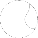
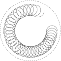
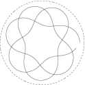
Figure 3: Vortex trajectories under the Collie-Tong flow on $\Sigma_{2,0}$. The curves show the trajectory of one of the vortices in each two vortex motion, and illustrate a variety of behaviours: (a) scattering, (b) an almost-circular bound orbit, (c) Larmor precession, (d) a cycloid-like bound orbit.

We can make a more complete analysis of the flow on $\Sigma_{n,n-1}$, since this is isometric to the hyperbolic plane of curvature $-1/3\pi n$, so $\kappa$ is constant. By rescaling $t$ we can scale away $\kappa$ in (5.4), so it suffices to consider the flow on, say, the hyperbolic plane of curvature $-1$. In the upper half plane model this has metric

$$\gamma=\frac{1}{y^{2}}(dx^{2}+dy^{2}).$$ (5.5)

To translate back to the disk model, we note that

$$\chi=\frac{z-i}{-iz+1},\qquad z=x+iy.$$ (5.6)

The vortex trajectories are then given by the $n$-th roots of $\chi(t)$. In the $z$ coordinate system (5.4) becomes

$$\ddot{x}-\frac{2}{y}\dot{x}\dot{y}+\dot{y} = 0,$$

$$\ddot{y}+\frac{1}{y}(\dot{x}^{2}-\dot{y}^{2})-\dot{x} = 0,$$ (5.7)

which has two conserved charges,

$$E=\frac{1}{2y^{2}}(\dot{x}^{2}+\dot{y}^{2}),\qquad P=\frac{\dot{x}-y}{y^{2}}.$$ (5.8)

Consider the trajectory with initial data $z(0)=i$, $\dot{z}(0)=iv$ for $v>0$. This has $P=-1$, so its projection to the $(y,\dot{y})$ phase plane is the energy level curve

$$\dot{y}^{2}=y^{2}(v^{2}-(1-y)^{2}).$$ (5.9)

For $0<v<1$ the trajectories are periodic, with $1-v\leq y(t)\leq 1+v$ while for $v\geq 1$ the trajectories are unbounded, escaping from and to the boundary at infinity ($y=0$) as $t\rightarrow\pm\infty$. Between critical points of $y(t)$, we can determine the trajectory $x(y)$ by solving

$$\frac{dx}{dy}=\frac{\dot{x}}{\dot{y}}=\pm\frac{1-y}{\sqrt{v^{2}-(1-y)^{2}}}.$$ (5.10)

One finds that

$$(x+v)^{2}+(y-1)^{2}=v^{2}$$ (5.11)

so the trajectory is a circle of radius $v$ centred on $(-v,1)$, or, if $v\geq 1$, the portion of this circle in the upper half plane. Note, in the latter case, that the trajectory intersects the boundary acutely, not orthogonally, though the trajectories tend to a geodesic as $v\rightarrow\infty$, as one would expect. By acting on this one-parameter family of circles with the isometry group of the hyperbolic plane ($SL(2,{\mathbb{R}})$ acting by fractional linear transformations, in the upper half plane model), we obtain all circles centred in the upper half plane (note that geodesics have centres on the boundary $y=0$). Under the Möbius transformation (5.6), these are mapped to circles with centres in the unit disk, and every such (arc of a) circle is a trajectory of the flow. The corresponding vortex trajectories in ${\mathsf{H}}$ (in the disk model) are then obtained by taking $n$-th roots. Clearly the behaviour is much simpler than that found numerically in $\Sigma_{2,0}$: all trajectories are either periodic or unbounded (both as $t\rightarrow\infty$ and $t\rightarrow-\infty$). Some examples are depicted in figure 4.

(a)	(b)	(c)	(d)

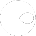
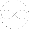
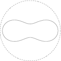
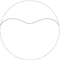
Figure 4: Vortex trajectories under the Collie-Tong flow on $\Sigma_{2,1}$. One vortex moves along the trajectory $\alpha(t)$ depicted, another moves along $-\alpha(t)$ while a third vortex remains stationary at the origin. In each case $\alpha(t)^{2}$ describes a circle with centre in the unit disk. In case $(b)$ this circle passes through $0$ so the vortices undergo $90^{\circ}$ scattering at the origin. The circle captures $0$ in cases (c) and (d), but not in case (a). Note that all trajectories are periodic or escape to infinity.

It would be interesting to make a systematic analysis of the flow (5.2) on a general Kähler manifold. One expects, for example, that the flow is complete if and only if the manifold is metrically complete. A natural generalization of the case $\Sigma_{n,n-1}$ considered in detail above would be to assume that ${\sf M}$ is a homogeneous Einstein manifold, for example ${\sf M}={\mathbb{C}}{{P}}^{N}$. This is potentially relevant to vortex dynamics on the two-sphere close to the Bradlow limit [1].

References

- [1] J. M. Baptista and N. S. Manton, The dynamics of vortices on S**2 near the Bradlow limit, J. Math. Phys. 44: 3495–3508 (2003), <hep-th/0208001>,
- [2] H. Y. Chen and N. S. Manton, The Kaehler potential of Abelian Higgs vortices, J. Math. Phys. 46 052305 (2005), <hep-th/0407011>,
- [3] B. Collie and D. Tong, The Dynamics of Chern-Simons Vortices, Phys. Rev. D78: 065013 (2008), <hep-th/0805.0602>,
- [4] Y. Kim and K. Lee, First and second order vortex dynamics, Phys. Rev. D66: 045016 (2002), <hep-th/0204111>,
- [5] S. Krusch and P. Sutcliffe, Schrödinger-Chern-Simons Vortex Dynamics, Nonlinearity 19: 1515–1534 (2006), <cond-mat/0511053>,
- [6] J. A. McGlade and J. M. Speight, Slow equivariant lump dynamics on the two-sphere, Nonlinearity 19: 441 (2006), <hep-th/0503086>,
- [7] N. S. Manton and P. Sutcliffe, Topological solitons, Cambridge University Press, Cambridge, U.K. (2004).
- [8] N. M. Romao, Ph.D. Thesis, University of Cambridge, 2002.
- [9] N. M. Romao, Dynamics of CP(1) lumps on a cylinder, J. Geom. Phys. 54: 42–76 (2005), <math-ph/0404008>,
- [10] T. M. Samols, Vortex scattering, Commun. Math. Phys. 145: 149–180 (1992),
- [11] I. A. B. Strachan, Low velocity scattering of vortices in a modified Abelian Higgs model, J. Math. Phys. 33: 102–110 (1992).