Phonon driven transport in amorphous semiconductors: Transition probabilities

Abstract

Inspired by Holstein’s work on small polaron hopping, the evolution equations of localized states and extended states in presence of atomic vibrations are derived for an amorphous semiconductor. The transition probabilities are obtained for four types of transitions: from one localized state to another localized state, from a localized state to an extended state, from an extended state to a localized state, and from one extended state to another extended state. At a temperature not too low, any process involving localized state is activated. The computed mobility of the transitions between localized states agrees with the observed ‘hopping mobility’. We suggest that the observed ‘drift mobility’ originates from the transitions from localized states to extended states. Analysis of the transition probability from an extended state to a localized state suggests that there exists a short-lifetime belt of extended states inside conduction band or valence band. It agrees with the fact that photoluminescence lifetime decreases with frequency in a-Si/SiO₂ quantum well while photoluminescence lifetime is not sensitive to frequency in c-Si/SiO₂ structure.

I Introduction

From the energy spectrum of an amorphous semiconductormd , one knows that there are four types of carrier transitions that may contribute to the electric conduction: type (1) transition between two localized states; type (2) transition from a localized state to an extended state; type (3) transition from an extended state to a localized state and type (4) transition between two extended states. Type (4) transition is common to both crystalline and non-crystalline materials. For amorphous semiconductors, type (1) transition is the main conduction mechanism in a broad temperature range. It has been investigated in various waysmul ; Over . Although the thermal equilibrium population of the extended states is lower than the population of the localized states, the contribution from the carriers in the extended states to the electric conduction is still observable for a moderately high temperature. An investigation of the transitions of type (2), type (3) and type (4) is necessary for a complete description of carrier dynamics.

In other electronic hopping processes, thermal vibrations of atoms also play an important role. Electron transfer (in polar solvent and inside large molecules)marcu and polaron diffusion in a molecular crystalHol1 ; Hol2 are two examples. The transition probability $W_{LL}$ between two sites in a thermally activated process is given by the Marcus formula

$$W_{LL}=\nu_{LL}e^{-E_{a}^{LL}/k_{B}T},\text{ \ }E_{a}^{LL}=\frac{\lambda_{LL}}{4}(1+\frac{\Delta G_{LL}^{0}}{\lambda_{LL}})^{2}$$ (1)

where $\nu_{LL}$ has the dimension of frequency for a specific hopping process. $E_{a}^{LL}$ is the temperature dependent activation energy. $\lambda_{LL}$ is the reorganization energy, $\Delta G_{LL}^{0}$ is the energy difference between the final state and the initial statemarcu . Eq.(1) is valid for both electron transfermarcu and small polaron hoppingrei . The mathematical form of Holstein’s work for one dimensional molecular crystal is quite flexible and can be used to treat three dimensional materials with slight modificationsEmin74 ; Emin75 ; Emin76 ; Emin77 ; Emin91 . The effect of static disorder may be taken into account by replacing a fixed transfer integral with a distribution. The static disorder reduces the strength of the electron-phonon (e-ph) coupling needed to stabilize global small-polaron fomationEmin94 . Amorphous semiconductors offer a different regime, in which the static disorder is so strong that the states in valence and conduction tails are localized. These localized states interact with the atomic vibrations.

We will extend Holstein’s workHol1 ; Hol2 to amorphous semiconductors. In Sec.II, we first introduce some notation about localized states, extended states and electron-phonon interaction. Then the equations of time evolution for localized states and extended states in presence of atomic vibrations are derived from a time-dependent Schrodinger equation. The connections with electron transfer, with Kramers’ problem of escape across a barrier and with small polarons are pointed out.

In Sec.III we study the hopping processes among localized states (LL) in amorphous solids. Eq.(1) is re-established in high temperature regime ($k_{B}T\gtrsim 2.5\hbar\overline{\omega},$ $\overline{\omega}=\int d\omega D(\omega)\omega/\int d\omega D(\omega)$ is the average phonon frequency, $D(\omega)$ is the spectral distribution of phonons, the factor 2.5 comes from the requirement that the error of approximation csch$\frac{\beta\hbar\overline{\omega}}{2}\thickapprox\frac{2k_{B}T}{\hbar\overline{\omega}}$ is less than 0.003, cf. the paragraph below Eq.(84)). The reorganization energy $\lambda_{LL}$ is expressed by the phonon spectrum, eigenvectors of the normal modes and the electron-phonon interaction parameters. The computed temperature dependence of the mobility of LL transition in a-Si agrees with that of the observed ‘hopping’ mobility for two regimes T$>$250K and T$<$250K (cf. Fig.1 and Fig.2).

The transition from a localized state to an extended state (LE) induced by the transfer integral is reported in Sec.IV, it has been suggested as the main conduction mechanism in amorphous silicon and is called ‘phonon induced delocalization’kik . Without the dressing effects of the vibrations of atoms, in certain sense, type (1) transition is similar to the transition between two bound states in a molecule and to the electron transfer between two ions, type (2) transition is analogous to the ionization process of an atom and to the escape across a potential barrier.

The transition from an extended state to a localized state (EL) induced by the electron-phonon interaction, is presented in Sec.V. In conduction band, the energy of an extended state is higher than that of a localized state in the lower tail. For an extended state with high enough energy, EL transition is in Marcus inverted regime. One expects that there exists a short-lifetime belt of the extended states inside conduction band or valence band (cf. Fig.3). The states inside this belt favor non-radiative transitions by emitting several phonons. The conjectured short-lifetime belt in conduction band agrees the fact that the photoluminescence lifetime of a-Si/SiO₂ quantum well decreases with frequency while that of c-Si/SiO₂ is not sensitive to frequency. Type (3) transition is similar to the free electron capture process in an atom and to the capture a particle by a well in a viscous liquid. One common feature of the type (1), (2) and (3) transitions is that at higher temperature $k_{B}T\gtrsim 2.5\hbar\overline{\omega}$, the probability of any transition involving localized state takes the form of Eq.(1). We suggest that the observed drift mobility may originate from type (2) transitions. Sec.VI is devoted to the transition between two extended states caused by electron-phonon interaction. Higher order processes and conduction mechanisms are briefly discussed. Finally we summarize this work and mention some un-touched problems.

II evolution of the states driven by the vibrations

II.1 Localized and extended states

Consider an amorphous sample with $\mathcal{N}$ atoms. Denote the static positions of the atoms as $\{\mathcal{R}_{\mathbf{n}},$ $\mathbf{n}=1,2,\cdots,\mathcal{N}\}$, the displacements of the atoms due to thermal vibrations as $\{\mathbf{u}^{\mathbf{n}},$ $\mathbf{n}=1,2,\cdots,\mathcal{N}\}$. To make the formulae compact, we rename the $3\mathcal{N}$ vibrational degrees of freedom $\{u_{x}^{1},u_{y}^{1},u_{z}^{1},\cdots,u_{x}^{\mathcal{N}},u_{y}^{\mathcal{N}},u_{z}^{\mathcal{N}}\}$ as $\{x_{k},$ $k=1,2,\cdots,3\mathcal{N}\}$ and rename the $3\mathcal{N}$ static position coordinates $\{\mathcal{R}_{1x},\mathcal{R}_{1y},\mathcal{R}_{1z},\cdots,\mathcal{R}_{\mathcal{N}x},\mathcal{R}_{\mathcal{N}y},\mathcal{R}_{\mathcal{N}z}\}$ as $\{X_{j},$ $j=1,2,\cdots,3\mathcal{N}\}$. Consider the single electron Hamiltonian:

$$h_{a}=-\frac{\hbar^{2}}{2m}\nabla^{2}+\sum_{\mathbf{n}=1}^{\mathcal{N}}U(\mathbf{r}-\mathcal{R}_{\mathbf{n}})$$ (2)

where $U(r-\mathcal{R}_{\mathbf{n}})$ is the potential energy felt by an electron at $\mathbf{r}$ due to an atom at $\mathcal{R}_{\mathbf{n}}$. In Eq.(2) only the static disorder of the amorphous sample is taken into account. $h_{a}$ is a mean field approximation, the existence of $U$ is known from Hartree-Fock method or density functional theory. $h_{a}$ has two kinds of eigenstates: localized states $\{\phi_{A_{1}}^{0}\}$

$$h_{a}\phi_{A_{1}}^{0}(\mathbf{r},\{\mathcal{R}_{\mathbf{n}}\})=E_{A_{1}}^{0}(\{\mathcal{R}_{\mathbf{n}}\})\phi_{A_{1}}^{0}(\mathbf{r},\{\mathcal{R}_{\mathbf{n}}\})$$ (3)

and extended states $\{\xi_{B_{1}}\}$

$$h_{a}\xi_{B_{1}}(\mathbf{r},\{\mathcal{R}_{\mathbf{n}}\})=E_{B_{1}}(\{\mathcal{R}_{\mathbf{n}}\})\xi_{B_{1}}(\mathbf{r},\{\mathcal{R}_{\mathbf{n}}\})$$ (4)

Eigenstates belonging to different eigenvalues are orthogonal to each other. In conduction band, the energies of the extended states are above those of the localized states. We use $A_{1},A_{2}\cdots=1,2,\cdots,N_{L}$ to label the localized states ($N_{L}$ is the total number of the localized states), $B_{1},B_{2}\cdots$ $=1,2,\cdots,N_{E}$ to label the extended states ($N_{E}$ is the total number of extended states).

When an electron in an extended state is scattered by phonons, the resulting state is still an extended state. The extended states are not radically modified by thermal vibrations. The situation for the localized states is different. The wave function of a localized state $\phi_{A_{1}}^{0}$ is non-zero only in some finite spatial region $D_{A_{1}}$: only the vibrations of the atoms inside $D_{A_{1}}$ couple to $\phi_{A_{1}}^{0}$:

$$\sum_{\mathbf{n}\in D_{A_{1}}}\int d\mathbf{r}\phi_{A_{1}}^{0\ast}[\mathbf{u}^{\mathbf{n}}\cdot\nabla_{\mathbf{n}}U(\mathbf{r}-\mathcal{R}_{\mathbf{n}})]\phi_{A_{1}}^{0}$$ (5)

The ‘concentrated’ wave function makes (5) comparable to or even larger than the transfer integral between two localized states and the transfer integral between a localized state and an extended state. The change in wave function of a localized state must be taken into account in the zeroth order:

$$[-\frac{\hbar^{2}}{2m}\nabla^{2}+\sum_{\mathbf{n}\in D_{A_{1}}}U(r-\mathcal{R}_{\mathbf{n}},\mathbf{u}^{\mathbf{n}})]\phi_{A_{1}}(\mathbf{r}-\mathcal{R}_{A_{1}},\{x_{p_{A_{1}}}^{A_{1}}\})=E_{A_{1}}(\{x_{p_{A_{1}}}^{A_{1}}\})\phi_{A_{1}}(\mathbf{r}-\mathcal{R}_{A_{1}},\{x_{p_{A_{1}}}^{A_{1}}\})$$ (6)

where $\mathcal{R}_{A_{1}}$ is a fixed point (could be arbitrarily chosen) inside $D_{A_{1}}$, $p_{A_{1}}$ is the index of the vibrational degrees of freedom inside $D_{A_{1}}$. Eq.(6) is a generalization of Eq.(I-3) in ref.Hol1, . The effect of the atoms in the neighboring regions of $D_{A_{1}}$ is neglected. The displacements of the atoms change the overlap integrals between localized states

$$T_{A_{2}A_{1}}=\int d^{3}r\phi_{A_{2}}^{\ast}(\mathbf{r}-\mathcal{R}_{A_{2}},\{x_{p_{A_{2}}}^{A_{2}}\})\phi_{A_{1}}(\mathbf{r}-\mathcal{R}_{A_{1}},\{x_{p_{A_{1}}}^{A_{1}}\})=\delta_{A_{2}A_{1}}+S_{A_{2}A_{1}}$$ (7)

For two localized states $A_{2}$ and $A_{1}$, $S_{A_{2}A_{1}}$ is a small quantity if $D_{A_{1}}$ and $D_{A_{2}}$ do not overlap. Using the linear approximation for e-ph interationHol1 ,

$$E_{A_{1}}(\{x_{p_{A_{1}}}^{A_{1}}\})=E_{A_{1}}^{0}-\sum_{p_{A_{1}}\mathbf{\in}D_{A_{1}}}d_{p_{A_{1}}}x_{p_{A_{1}}}^{A_{1}},\text{ \ \ \ \ }d_{p_{A_{1}}}=\int d\mathbf{r}\phi_{A_{1}}^{0}(\mathbf{r},\{\mathcal{R}_{\mathbf{n}}\})\frac{\partial U}{\partial X_{p_{A_{1}}}}\phi_{A_{1}}^{0}(\mathbf{r},\{\mathcal{R}_{\mathbf{n}}\})$$ (8)

Eq.(8) is the first order correction of electronic energy due to the e-ph interaction. The most localized states can be described by $\xi^{-3/2}e^{-r/\xi},$ where $\xi$ is localization length of a localized state, $r$ is the distance between electron and some representative point inside $D_{A_{1}}$. $d_{p_{A_{1}}}\thicksim\frac{Z^{\ast}e^{2}}{4\pi\epsilon_{0}\xi^{2}},$ $\epsilon_{0}$ is the permittivity of vacuum, $Z^{\ast}$ is the effective nuclear charge of an atom felt by a conduction electron. For electrons in a metal, researchers usually focus on how an electron in an extended state is scattered into another extended state by the e-ph interaction rather than the correction to energy. Unlike $\phi_{A_{1}}^{0}$, $\phi_{A_{1}}$ includes the effect of vibrations of the atoms and is no longer orthogonal to any extended states of (2),

$$\int d^{3}r\xi_{B_{2}}^{\ast}(\mathbf{r},\{\mathcal{R}_{\mathbf{n}}\})\phi_{A_{1}}(\mathbf{r}-\mathcal{R}_{A_{1}},\{x_{p_{A_{1}}}^{A_{1}}\})=Y_{B_{2}A_{1}}$$ (9)

II.2 Single-electron approximation

For definiteness, we consider the electrons in the conduction band of an amorphous semiconductor. For carriers in the mid-gap states and the holes in valence band, we need only slightly modify the notation. In intrinsic and lightly doped n-type semiconductors, the number of the electrons is much smaller than the number of the localized states. The correlation between electrons in a hopping process and the screen effect caused by these electrons can be neglected. Essentially we have a single particle problem: one electron moves in many empty localized states and extended states in the conduction band.

Consider one electron moving in an amorphous solid with $\mathcal{N}$ atoms, the total Hamiltonian of the system is

$$H=\frac{-\hbar^{2}}{2m}\nabla^{2}+\sum_{\mathbf{n}=1}^{\mathcal{N}}U(\mathbf{r},\mathbf{W}_{\mathbf{n}})+\sum_{\mathbf{n}}\frac{-\hbar^{2}}{2M_{\mathbf{n}}}\nabla_{\mathbf{n}}^{2}+\sum_{\mathbf{n,n}^{\prime}\mathbf{(n\neq n}^{\prime})}V(\mathbf{W}_{\mathbf{n}},\mathbf{W}_{\mathbf{n}^{\prime}})$$ (10)

where $\mathbf{n}$ denote the site of network, $\mathbf{W}_{\mathbf{n}}$ is the instantaneous position vector of the nucleus at site $\mathbf{n}$, $U(\mathbf{r},\mathbf{W}_{\mathbf{n}})$ is the interaction between the electron and the nucleus at the $\mathbf{n}^{\text{th}}$ site. $V(\mathbf{W}_{\mathbf{n}},\mathbf{W}_{\mathbf{n}^{\prime}})$ is the total effective interaction of the nucleus at site $\mathbf{n}^{\prime}$ and the nucleus at site $\mathbf{n},$ which including both the Coulomb repulsion between them and the induced attraction by the electrons. The total wave function $\psi(\mathbf{r},\{\mathbf{W}_{\mathbf{n}}\};t)$ of the system is a function of all degrees of freedom, its time evolution is determined by

$$i\hbar\frac{\partial}{\partial t}\psi(\mathbf{r},\{\mathbf{W}_{\mathbf{n}}\};t)=H\psi(\mathbf{r},\{\mathbf{W}_{\mathbf{n}}\};t)\text{.}$$ (11)

For temperature well below melting point, the system executes small harmonic oscillations. The motion of nuclei $\mathbf{W}_{\mathbf{n}}=\mathcal{R}_{\mathbf{n}}+\mathbf{u}^{\mathbf{n}}$ can be viewed as vibrations of the atoms $\{\mathbf{u}^{\mathbf{n}}\}$ around their equilibrium positions $\{\mathcal{R}_{\mathbf{n}}\}$. $\psi(\mathbf{r},\{\mathbf{W}_{\mathbf{n}}\};t)$ is changed into $\psi(\mathbf{r},\{\mathbf{u}^{\mathbf{n}}\};t)$, a function of displacements of the atoms. $H$ is simplified as

$$H_{1}=h_{e}+h_{v}$$ (12)

where

$$h_{e}=\frac{-\hbar^{2}}{2m}\nabla^{2}+\sum_{\mathbf{n}=1}^{\mathcal{N}}U(\mathbf{r},\mathcal{R}_{\mathbf{n}},\mathbf{u}^{\mathbf{n}}),\text{ \ \ }h_{v}=\sum_{j}-\frac{\hbar^{2}}{2M_{j}}\nabla_{j}^{2}+\frac{1}{2}\sum_{jk}k_{jk}x_{j}x_{k}$$ (13)

$h_{e}$ is the single electron Hamiltonian including the vibrations. $h_{a}$ in Eq.(2) and the Hamiltonian in Eq.(6) are two different approximations of $h_{e}$. $h_{v}$ is the vibrational Hamiltonian, $(k_{jk})$ is the matrix of force constants. The evolution of the total wave function $\psi(\mathbf{r},\{\mathbf{u}^{\mathbf{n}}\};t)$ of the system of “one electron + many nuclei” is given by Schrodinger equation

$$i\hbar\frac{\partial\psi(\mathbf{r},\{\mathbf{u}^{\mathbf{n}}\};t)}{\partial t}=H_{1}\psi(\mathbf{r},\{\mathbf{u}^{\mathbf{n}}\};t)$$ (14)

II.3 Evolution equations

The Hilbert space of $h_{e}$ is spanned by the localized states and the extended states. The total wave function $\psi(\mathbf{r},\{\mathbf{u}^{\mathbf{n}}\};t)$ of the system of “one electron + many nuclei” can be expanded as

$$\psi(\mathbf{r},x_{1},\cdots,x_{3\mathcal{N}};t)=\sum_{A_{1}}a_{A_{1}}(x_{1},\cdots,x_{3\mathcal{N}};t)\phi_{A_{1}}+\sum_{B_{1}}b_{B_{1}}(x_{1},\cdots,x_{3\mathcal{N}};t)\xi_{B_{1}}$$ (15)

where $a_{A_{1}}$ is the probability amplitude at moment $t$ that the electron is in localized state $A_{1}$ while the displacements of the nuclei are $\{x_{j},$ $j=1,2,\cdots 3\mathcal{N}\}$, $b_{B_{1}}$ is the amplitude at moment $t$ that the electron is in extended state $B_{1}$ while the displacements of the nuclei are $\{x_{j},$ $j=1,2,\cdots 3\mathcal{N}\}$. The first sum runs over all the localized states, the second sum runs over all the extended states. Substitute Eq.(15) into Eq.(14), we have

$$\sum_{A_{1}}i\hbar\frac{\partial a_{A_{1}}}{\partial t}\phi_{A_{1}}+\sum_{B_{1}}i\hbar\frac{\partial b_{B_{1}}}{\partial t}\xi_{B_{1}}=\sum_{A_{1}}a_{A_{1}}E_{A_{1}}\phi_{A_{1}}+\sum_{A_{1}}a_{A_{1}}\sum_{\mathbf{p}\notin D_{A_{1}}}U(r-\mathcal{R}_{\mathbf{p}},\mathbf{u}_{\mathbf{p}})\phi_{A_{1}}$$ (16)

$$+\sum_{A_{1}}\phi_{A_{1}}h_{v}a_{A_{1}}+\sum_{A_{1}}\sum_{j}-\frac{\hbar^{2}}{M_{j}}(\nabla_{j}a_{A_{1}})(\nabla_{j}\phi_{A_{1}})+\sum_{A_{1}}\sum_{j}-\frac{\hbar^{2}}{2M_{j}}a_{A_{1}}\nabla_{j}^{2}\phi_{A_{1}}$$

$$+\sum_{B_{1}}b_{B_{1}}E_{B_{1}}\xi_{B_{1}}+\sum_{B_{1}}b_{B_{1}}\sum_{j}x_{j}\frac{\partial U}{\partial X_{j}}\xi_{B_{1}}+\sum_{B_{1}}\xi_{B_{1}}\sum_{j}h_{v}b_{B_{1}}$$

$$+\sum_{B_{1}}\sum_{j}-\frac{\hbar^{2}}{M_{j}}(\nabla_{j}b_{B_{1}})(\nabla_{j}\xi_{B_{1}})+\sum_{B_{1}}\sum_{j}-\frac{\hbar^{2}}{2M_{j}}b_{B_{1}}\nabla_{j}^{2}\xi_{B_{1}}$$

In extended states $\{\xi_{B_{1}}\}$, we neglected the dependence of on the vibrational displacements, the last two terms disappear.

Differences between the localized states and the extended states are reflected in Eq.(16). For a localized state, we have separated

$$\sum_{\mathbf{n}}U(r-\mathcal{R}_{\mathbf{n}},\mathbf{u}^{\mathbf{n}})=\sum_{\mathbf{n}\in D_{A_{1}}}U(r-\mathcal{R}_{\mathbf{n}},\mathbf{u}^{\mathbf{n}})+\sum_{\mathbf{p}\notin D_{A_{1}}}U(r-\mathcal{R}_{\mathbf{p}},\mathbf{u}^{\mathbf{p}})$$ (17)

the second term leads to the transfer integral which causes transition among states. The wave function of localized state $A_{1}$ is confined in $D_{A_{1}}$. For a nucleus outside $D_{A_{1}}$, its effect on $A_{1}$ dies away with the distance between the nucleus and $D_{A_{1}}$. Eq.(17) is a generalization of Holstein’s treatmentHol1 to a localized state which occupies several sites. While for extended states we have resolved

$$\sum_{\mathbf{n}}U(r-\mathcal{R}_{\mathbf{n}},\mathbf{u}^{\mathbf{n}})=\sum_{\mathbf{n}=1}^{\mathcal{N}}U(\mathbf{r}-\mathcal{R}_{\mathbf{n}})+\sum_{j=1}^{3\mathcal{N}}x_{j}\frac{\partial U}{\partial X_{j}}$$ (18)

the second term is the electron-phonon interaction. An extended state spreads over whole sample, it feels the vibrations of all the atoms. Eq.(18) is similar to the usual treatment of e-ph interaction in a crystal.

The first sum in Eq.(17) only includes the atoms in the region where the wave function of localized state $A_{1}$ is nonzero. If a localized state is close to mobility edge, it extends to a very large spatial region. For such a state, Eq.(17) is not very different from Eq.(18).

By applying $\int d^{3}r\phi_{A_{2}}^{\ast}$ to both sides of Eq.(16), one obtains:

$$\sum_{A_{1}}T_{A_{2}A_{1}}\{i\hbar\frac{\partial}{\partial t}-E_{A_{1}}-h_{v}\}a_{A_{1}}+\sum_{B_{1}}Y_{A_{2}B_{1}}^{\ast}\{i\hbar\frac{\partial}{\partial t}-E_{B_{1}}-h_{v}\}b_{B_{1}}=$$ (19)

$$\sum_{A_{1}}a_{A_{1}}\int d^{3}r\phi_{A_{2}}^{\ast}\sum_{\mathbf{p}\notin D_{A_{1}}}U(r-\mathcal{R}_{\mathbf{p}},\mathbf{u}_{\mathbf{p}})\phi_{A_{1}}+\sum_{B_{1}}b_{B_{1}}\int d^{3}r\phi_{A_{2}}^{\ast}\sum_{j}x_{j}\frac{\partial U}{\partial X_{j}}\xi_{B_{1}}$$

$$+\sum_{A_{1}}\sum_{j}-\frac{\hbar^{2}}{M_{j}}(\nabla_{j}a_{A_{1}})\int d^{3}r\phi_{A_{2}}^{\ast}(\nabla_{j}\phi_{A_{1}})+\sum_{A_{1}}\sum_{j}-\frac{\hbar^{2}}{2M_{j}}a_{A_{1}}\int d^{3}r\phi_{A_{2}}^{\ast}\nabla_{j}^{2}\phi_{A_{1}}$$

Application of $\int d^{3}r\xi_{B_{2}}^{\ast}$ to both sides of Eq.(16) yields:

$$\sum_{A_{1}}Y_{B_{2}A_{1}}\{i\hbar\frac{\partial}{\partial t}-E_{A_{1}}-h_{v}\}a_{A_{1}}+\{i\hbar\frac{\partial}{\partial t}-E_{B_{2}}-h_{v}\}b_{B_{2}}$$ (20)

$$=\sum_{A_{1}}a_{A_{1}}\sum_{\mathbf{p}\notin D_{A_{1}}}\int d^{3}r\xi_{B_{2}}^{\ast}U(r-\mathcal{R}_{\mathbf{p}},\mathbf{u}^{\mathbf{p}})\phi_{A_{1}}+\sum_{B_{1}}b_{B_{1}}\sum_{j}x_{j}\int d^{3}r\xi_{B_{2}}^{\ast}\frac{\partial U}{\partial X_{j}}\xi_{B_{1}}$$

$$+\sum_{A_{1}}\sum_{j}-\frac{\hbar^{2}}{M_{j}}(\nabla_{j}a_{A_{1}})\int d^{3}r\xi_{B_{2}}^{\ast}(\nabla_{j}\phi_{A_{1}})+\sum_{A_{1}}\sum_{j}-\frac{\hbar^{2}}{2M_{j}}a_{A_{1}}\int d^{3}r\xi_{B_{2}}^{\ast}\nabla_{j}^{2}\phi_{A_{1}}$$

The coupled equations Eq.(19) and Eq.(20) describe the time evolution of the states under the influence of the vibrations: the transition between two localized states (LL), the transition between two extended states (EE), the transition from an extended state to a localized state (EL) and the transition from a localized state to an extended state (LE). In other words, for a given initial state, i.e. $\{a_{A_{1}}(x_{1},\cdots,x_{3\mathcal{N}};t=0),A_{1}=1,2,\cdots,N_{L}\}$ and $\{b_{B_{1}}(x_{1},\cdots,x_{3\mathcal{N}};t=0),B_{1}=1,2,\cdots,N_{E}\}$, at any subsequent moment $t>0$ the state of the system is completely determined (i.e $\{a_{A_{1}}(x_{1},\cdots,x_{3\mathcal{N}};t),A_{1}=1,2,\cdots,N_{L}\}$ and $\{b_{B_{1}}(x_{1},\cdots,x_{3\mathcal{N}};t),B_{1}=1,2,\cdots,N_{E}\}$) by Eqs. (19) and (20). The number of vibrational degrees of freedom is macroscopic, so that $\{a_{A_{1}}(t=0),A_{1}=1,2,\cdots,N_{L}\}$ and $\{b_{B_{1}}(t=0,B_{1}=1,2,\cdots,N_{E}\}$ cannot be assigned precisely. A description based on density matrix is more appropriate.

Let us estimate the order of magnitude of the last two terms in RHS of Eq.(19) or Eq.(20). From the 1${}^{\text{st}}$ order perturbation correction about the nuclear displacements to the localized wave function, we have

$$\nabla_{j}\phi_{A_{1}}=\sum_{C}{}^{\prime}\frac{\langle C|\sum_{j\in A_{1}}\frac{\partial U}{\partial X_{j}}|A_{1}\rangle}{E_{A_{1}}-E_{C}}|C\rangle\thicksim\frac{U}{\hbar v_{e}}$$ (21)

where $v_{e}$ is a typical velocity of electron, $C$ is eigenvalue $A$ or $B$ of $h_{a}$. To reach last step, we notice the derivative of $U(\mathbf{r}-\mathcal{R}_{j})$ respect to suitable coordinate component of electron equals $-\frac{\partial U}{\partial X_{j}}$. Thus $\frac{\partial U}{\partial X_{j}}\thicksim p_{e}U/\hbar$, $p_{e}$ is momentum of the electron, and $v_{e}=\frac{\Delta E}{\Delta p_{e}}$. A typical term in the 2${}^{\text{nd}}$ sum from last in RHS of Eq.(19) becomes

$$\frac{\hbar^{2}}{M_{j}}\nabla_{j}a_{A_{1}}\cdot\nabla_{j}\phi_{A_{1}}\text{ }\thicksim\frac{v_{n}}{v_{e}}U\text{ }$$ (22)

where $v_{n}\thicksim M_{j}^{-1}\hbar\nabla_{j}$ is typical velocity of a nucleus. A typical term in the last sum in RHS of Eq.(19) can be estimated from 2nd order correction to $\phi_{A_{1}}$ about the nuclear displacements

$$\frac{\hbar^{2}}{2M_{j}}\nabla_{j}^{2}\phi_{A_{1}}\thicksim\frac{U^{2}}{Mv_{e}^{2}}\thicksim\frac{m}{M}U$$ (23)

In the last $\thicksim$, we applied the virial theorem $mv_{e}^{2}\thicksim U$, $m$ is the mass of electron, $U$ is the interaction potential energy between electron and some nucleus. Clearly

$$x_{j}\frac{\partial U}{\partial X_{j}}\thicksim\frac{x}{d}U$$ (24)

where $x$ is a typical vibrational amplitude of atoms, $d$ is the distance between two nearest neighbor atoms. Notice $v_{n}/v_{e}\thicksim 10^{-3}$, $m/M\thicksim 10^{-4}$ and $x/d\thicksim 10^{-2}-10^{-1}$, combining Eqs. (22), (23) and (24), we find

$$\sum_{j}\frac{\hbar^{2}}{M_{j}}(\nabla_{j}a_{A_{1}})(\nabla_{j}\phi_{A_{1}})\text{ or }\sum_{j}\frac{\hbar^{2}}{2M_{j}}\nabla_{j}^{2}\phi_{A_{1}}<<\sum_{\mathbf{p}\notin D_{A_{1}}}U(r-\mathcal{R}_{\mathbf{p}},\mathbf{u}^{\mathbf{p}})\phi_{A_{1}}\text{ or }\sum_{j}x_{j}\frac{\partial U}{\partial X_{j}}\xi_{B_{1}}$$ (25)

The 3rd term and the 4th term in the RHS of both Eq.(19) and Eq.(20) can be ignored. Eq.(19) is reduced to

$$\sum_{A_{1}}T_{A_{2}A_{1}}\{i\hbar\frac{\partial}{\partial t}-E_{A_{1}}-h_{v}\}a_{A_{1}}+\sum_{B_{1}}Y_{A_{2}B_{1}}^{\ast}\{i\hbar\frac{\partial}{\partial t}-E_{B_{1}}-h_{v}\}b_{B_{1}}=$$ (26)

$$\sum_{A_{1}}a_{A_{1}}\int d^{3}r\phi_{A_{2}}^{\ast}\sum_{\mathbf{p}\notin D_{A_{1}}}U(r-\mathcal{R}_{\mathbf{p}},\mathbf{u}^{\mathbf{p}})\phi_{A_{1}}+\sum_{B_{1}}b_{B_{1}}\int d^{3}r\phi_{A_{2}}^{\ast}\sum_{j}x_{j}\frac{\partial U}{\partial X_{j}}\xi_{B_{1}}$$

In the right hand side (RHS), each term in the first sum is a transition between two localized states mediated by a transfer integral. Each term in the second sum is a transition from an extended state to a localized state caused by the electron-phonon interaction. Similarly Eq.(20) is reduced to

$$\sum_{A_{1}}Y_{B_{2}A_{1}}\{i\hbar\frac{\partial}{\partial t}-E_{A_{1}}-h_{v}\}a_{A_{1}}+\{i\hbar\frac{\partial}{\partial t}-E_{B_{2}}-h_{v}\}b_{B_{2}}=$$ (27)

$$\sum_{A_{1}}a_{A_{1}}\sum_{\mathbf{p}\notin D_{A_{1}}}\int d^{3}r\xi_{B_{2}}^{\ast}U(r-\mathcal{R}_{\mathbf{p}},\mathbf{u}^{\mathbf{p}})\phi_{A_{1}}+\sum_{B_{1}}b_{B_{1}}\sum_{j}x_{j}\int d^{3}r\xi_{B_{2}}^{\ast}\frac{\partial U}{\partial X_{j}}\xi_{B_{1}}$$

In the RHS, each term in the first sum is a transition from a localized state to an extended state induced by a transfer integral. Each term in the second sum is a transition between two extended states caused by electron-phonon interaction.

Eqs.(26) and (27) are completely general. To simplify them we need two connected technical assumptions (i) $Y_{B_{2}A_{1}}\thicksim\frac{N_{A_{1}}}{\mathcal{N}}<<1$ and (ii) $S_{A_{2}A_{1}}<<1$. Obviously they are not true in general. For localized states which are close to mobility edge, they spread in many distorted spatial regions. The overlap integral $Y_{B_{2}A_{1}}$ between them and an extended state is not small (when e-ph interaction appears, they are no longer eigenstates of $h_{a}$). Assumption (i) means that we do not consider the localized states very close to mobility edge and consider only the most localized states. The contributions to conductivity from near-edge localized states are ignored. For the most localized states (the most low-lying ones in conduction band), which spread over only several bond lengths at most, condition (i) is satisfied. Condition (ii) is satisfied for two localized states which do not overlap. It means we exclude the indirect contribution to conductivity from the transitions between two localized states with overlapping spatial regions. For two eigenstates $A_{2}$ and $A_{1}$ of static hamiltonian $h_{a}$, the overlap integral between two states $S_{A_{2}A_{1}}=0.$ In addition, if the distance between two localized states is larger than one bond length, the overlap integral can be neglected even one takes into account electron-phonon interaction (e-ph). When e-ph interaction is taken into account, $A_{2}$ and $A_{1}$ are no longer eigenstates of $h_{a}$, $S_{A_{2}A_{1}}$ is not negligible when the spatial regions of two localized states overlap. For a localized state which spreads in several distorted regionsdong ; lud , its wave function is not single exponential decay function which is only suitable for the most localized statesbig . The overlap integrals $Y_{B_{2}A_{1}}$ and $S_{A_{2}A_{1}}$ involving such a localized state are oscillatory. To make a semi-classical estimation, one needs detailed information of wavefunction which could be obtained through a WKB-like exponential transform. We wish to remove two assumptions in a later communicationwkb .

The transition between two localized states is significant only when the distance $R_{12}$ between the two is not very large. For two localized states $A_{2}$ and $A_{1}$, $S_{A_{2}A_{1}}<<1$ if $D_{A_{1}}$ and $D_{A_{2}}$ do not overlap. The terms multiplied by $S_{A_{2}A_{1}}$ can be neglected for localized states which their spatial regions do not overlap. What is more, the transfer integral is important only when the atoms $\mathbf{p}\notin D_{A_{1}}$ fall into $D_{A_{2}}$ or $A_{1}=A_{2}$,

$$\sum_{A_{1}}a_{A_{1}}\int d^{3}r\phi_{A_{2}}^{\ast}\sum_{\mathbf{p}\notin D_{A_{1}}}U(r-\mathcal{R}_{\mathbf{p}},\mathbf{u}^{\mathbf{p}})\phi_{A_{1}}\thickapprox\sum_{A_{1}}a_{A_{1}}J_{A_{2}A_{1}}+W_{A_{2}}a_{A_{2}}\thickapprox\sum_{A_{1}}a_{A_{1}}J_{A_{2}A_{1}}$$ (28)

where

$$J_{A_{2}A_{1}}=\int d^{3}r\phi_{A_{2}}^{\ast}\sum_{\mathbf{p}\in D_{A_{2}}}U(r-\mathcal{R}_{\mathbf{p}},\mathbf{u}^{\mathbf{p}})\phi_{A_{1}},\text{ \ \ \ }W_{A_{2}}=\int d^{3}r|\phi_{A_{2}}|^{2}\sum_{\mathbf{p}\notin D_{A_{2}}}U(r-\mathcal{R}_{\mathbf{p}},\mathbf{u}^{\mathbf{p}})$$ (29)

Here, the $W_{A_{2}}$ term only affects the self energy of a localized state through $a_{A_{2}}$. Eqs.(28) and (29) are a generalization of Eqs.(I-14) to (I-16) of ref.Hol1, . Comparing with $E_{A_{1}}$ and with $h_{v}$, $W_{A_{2}}$ can be neglected. $J_{A_{2}A_{1}}$ causes the transition from $A_{1}$ to $A_{2}$, it comes from the attraction on the electron by the atoms in $D_{A_{2}}$. For those most localized states, the wave functions take form of $\phi_{A_{1}}\thicksim e^{-|\mathbf{r}-\mathcal{R}_{A_{1}}|/\xi_{1}}$. $J_{A_{2}A_{1}}$ is estimated to bepau $-\frac{N_{A_{2}}Z^{\ast}e^{2}}{4\pi\epsilon_{0}\varepsilon_{s}\xi}(1+\frac{R_{12}}{\xi})e^{-R_{12}/\xi}$, where average localization length $\xi$ is defined by $2\xi^{-1}=\xi_{1}^{-1}+\xi_{2}^{-1}$. $R_{12}$ is the average distance between two localized states, $\varepsilon_{s}$ is static dielectric function, $Z^{\ast}$ is the effective nuclear charge of atom, $N_{A_{2}}$ is the number of atoms inside region $D_{A_{2}}$.

Similarly $J_{A_{1}A_{2}}$ causes the transition from $A_{2}$ to $A_{1}$, it comes from the attraction on the electron by the atoms in $D_{A_{1}}$. For two localized states $A_{1}$ and $A_{2}$ in different regions, no simple relation exists between $J_{A_{2}A_{1}}$ and $J_{A_{1}A_{2}}$. This is in contrast with the situation $J_{A_{2}A_{1}}=(J_{A_{1}A_{2}})^{\ast}$ of small polarons in crystal where translational invariance exists Hol2 . Later we neglect the dependence of $J_{A_{2}A_{1}}$ on the displacements $\{x\}$ of the atoms and consider $J_{A_{2}A_{1}}$ as a function of the distance $R_{12}$ between two localized states, localization length $\xi_{1}$ of state $A_{1}$ and localization length $\xi_{2}$ of state $A_{2}$.

Eqs.(26) and (27) are then reduced to

$$\{i\hbar\frac{\partial}{\partial t}-E_{A_{2}}-h_{v}\}a_{A_{2}}+\sum_{B_{1}}Y_{A_{2}B_{1}}^{\ast}\{i\hbar\frac{\partial}{\partial t}-E_{B_{1}}-h_{v}\}b_{B_{1}}=\sum_{A_{1}}J_{A_{2}A_{1}}a_{A_{1}}+\sum_{B_{1}}K_{A_{2}B_{1}}^{\prime}b_{B_{1}}$$ (30)

and

$$\sum_{A_{1}}Y_{B_{2}A_{1}}\{i\hbar\frac{\partial}{\partial t}-E_{A_{1}}-h_{v}\}a_{A_{1}}+\{i\hbar\frac{\partial}{\partial t}-E_{B_{2}}-h_{v}\}b_{B_{2}}=\sum_{A_{1}}J^{\prime}{}_{B_{2}A_{1}}a_{A_{1}}+\sum_{B_{1}}K_{B_{2}B_{1}}b_{B_{1}}$$ (31)

where

$$K_{A_{2}B_{1}}^{\prime}=\sum_{j}x_{j}\int d^{3}r\phi_{A_{2}}^{\ast}\frac{\partial U}{\partial X_{j}}\xi_{B_{1}}$$ (32)

is a linear function of atomic displacements $x_{j}$. It causes type (3) transition from an extended state to a localized state. If we approximate extended state as plane wave $\xi_{B_{1}}\thicksim e^{ik_{B_{1}}r}$, $K_{A_{2}B_{1}}^{\prime}\thicksim\frac{Z^{\ast}e^{2}u}{4\pi\epsilon_{0}\varepsilon_{s}\xi_{A_{2}}^{2}}(1-ik_{B_{1}}\xi_{A_{2}})^{-1}$, where $u\thicksim\sqrt{\frac{k_{B}T}{M\omega^{2}}}$ or $\sqrt{\frac{\hbar}{M\omega}}$ is typical amplitude of vibration at high or low temperature. So that $K_{A_{2}B_{1}}^{\prime}u/J_{A_{2}A_{1}}\thicksim e^{R_{12}/\xi}u/\xi$. The distance between two nearest localized states is about several Å in a-Si, $K_{A_{2}B_{1}}^{\prime}u$ is several times smaller than $J_{A_{2}A_{1}}$.

From Eqs.(30) and (31), type (2) transition from a localized state in region $D_{A_{1}}$ to an extended state is caused by the transfer integral

$$J^{\prime}{}_{B_{2}A_{1}}=\sum_{\mathbf{p}\notin D_{A_{1}}}\int d^{3}r\xi_{B_{2}}^{\ast}U(r-\mathcal{R}_{\mathbf{p}},\mathbf{u}^{\mathbf{p}})\phi_{A_{1}}$$ (33)

not by the electron-phonon interaction $K_{A_{2}B_{1}}^{\prime}$ (although we will see the process does involve several phonons in high temperature regime in Sec.IV, it consists with the intuitive picture of ‘phonon induced delocalization’kik ). $J^{\prime}{}_{B_{2}A_{1}}$ does not involve atomic displacements explicitly. Later we neglect the dependence of $J^{\prime}{}_{B_{2}A_{1}}$ on the displacements of atoms and only view $J^{\prime}{}_{B_{2}A_{1}}$ as function of $\xi_{A_{1}}$ only. If we approximate extended state as plane wave $\xi_{B_{2}}^{\ast}\thicksim e^{-ik_{B_{2}}r}$, $J^{\prime}{}_{B_{2}A_{1}}\thicksim\frac{Z^{\ast}e^{2}}{4\pi\epsilon_{0}\varepsilon_{s}\xi_{A_{1}}}(1+ik_{B_{2}}\xi_{A_{1}})^{-2}$. $J^{\prime}{}_{B_{2}A_{1}}$ is in the same order of magnitude as $J_{A_{2}A_{1}}$. According to Eqs.(30) and (31), $J^{\prime}{}_{B_{2}A_{1}}$ does not create transitions from an extended state to a localized state. The asymmetries in Eq.(32) and Eq.(33) come from the different separations Eq.(17) and Eq.(18) of the single particle potential energy for localized states and extended states. One should not confuse with the usual symmetry between transition probabilities for forward process and backward process computed by the first order perturbation theory, where two processes are coupled by the same interaction.

Type (4) transition between two extended states $B_{1}$ and $B_{2}$ is caused by electron-phonon interaction:

$$K_{B_{2}B_{1}}=\sum_{j}x_{j}\int d^{3}r\xi_{B_{2}}^{\ast}\frac{\partial U}{\partial X_{j}}\xi_{B_{1}},\text{ \ \ \ }K_{B_{2}B_{1}}=(K_{B_{1}B_{2}})^{\ast}$$ (34)

It is almost the same as the usual scattering between two Bloch states in a crystal by the electron-phonon interaction. If we approximate extended states $\xi_{B_{1}}$ and $\xi_{B_{2}}$ by plane waves with wave vector $k_{1}$ and $k_{2}$, $K_{B_{2}B_{1}}\thicksim\frac{Z^{\ast}e^{2}u\kappa^{3}}{4\pi\epsilon_{0}\varepsilon_{s}[\kappa+i(k_{2}-k_{1})]}$, where $\kappa\thicksim\frac{e^{2}}{\epsilon_{0}}\frac{\partial n}{\partial\mu}$ is the Thomas-Fermi screening wave vector. In lightly doped or intrinsic semiconductor, $\kappa$ is hundreds even thousands times smaller than $1/a,$ $a$ is bond length. Since for most localized state, localization length $\xi$ is several times $a$, $K_{B_{2}B_{1}}\thicksim(\kappa\xi)^{2}K_{A_{2}B_{1}}^{\prime}$, is much weaker than three other coupling constants. Contrast with type (1), type (2) and type (3) transitions, the transition probability of the transition $B_{1}\rightarrow B_{2}$ equals to $B_{2}\rightarrow B_{1}$: two processes are coupled by the same interaction as illustrated in Eq.(34). Eq.(30) and Eq.(31) correspond to the generalized master equation for the reduced density matrix of an electron in a phonon bathmas .

In the conduction band of an amorphous solid, the energies of extended states are higher than the energies of  the localized states close to the bottom of the band. If a localized state is not very close to the mobility edge, its localization length $\xi$ is small. The overlap between it and an extended state $Y_{B_{2}A_{1}}\thicksim\frac{N_{A_{1}}}{\mathcal{N}}$ may be neglected. Eq.(30) and Eq.(31) read as

$$\{i\hbar\frac{\partial}{\partial t}-E_{A_{2}}-h_{v}\}a_{A_{2}}=\sum_{A_{1}}J_{A_{2}A_{1}}a_{A_{1}}+\sum_{B_{1}}K_{A_{2}B_{1}}^{\prime}b_{B_{1}}$$ (35)

and

$$\{i\hbar\frac{\partial}{\partial t}-E_{B_{2}}-h_{v}\}b_{B_{2}}=\sum_{A_{1}}J^{\prime}{}_{B_{2}A_{1}}a_{A_{1}}+\sum_{B_{1}}K_{B_{2}B_{1}}b_{B_{1}}$$ (36)

If a localized state is close to the mobility edge, the overlaps between it and the extended states are not necessarily small. Eqs. (35) and (36) could be used generically with the restrictions (i) and (ii).

In Eq.(35) and Eq.(36), the e-ph interaction for localized state and extended state has been treated differently. The reason is as following. Let us consider the potential energy of atoms

$$\frac{1}{2}\sum_{jk}k_{jk}x_{j}x_{k}-\sum_{p}g_{p}x_{p},\text{ \ \ \ }g_{p}=-\frac{\partial U}{\partial X_{p}}$$ (37)

the first term is the mutual interactions among atoms. The second term, the e-ph interaction, acts like an external field. The first member of Eq.(37) can be written as:

$$\frac{1}{2}\sum_{jk}k_{jk}(x_{j}-x_{j}^{0})(x_{k}-x_{k}^{0})-\frac{1}{2}\sum_{jk}k_{jk}x_{j}^{0}x_{k}^{0}$$ (38)

where

$$\text{\ }x_{m}^{0}=\sum_{p}(k^{-1})_{mp}g_{p},m=1,2,\cdots 3\mathcal{N}$$ (39)

is the static displacement for the $m^{\text{th}}$ degree of freedom. The constant force $-\frac{\partial U}{\partial X_{p}}$ exerted by electron on the $p^{\text{th}}$ vibrational degree of freedom produces a static displacement $x_{m}^{0}$ for the $m^{\text{th}}$ degree of freedom. The deformation caused by the static external force of e-ph interaction is balanced by the elastic force. A similar result was obtained for continuum modelEmin76 . The last term in Eq.(38) is the polarization energy, a combined contribution from elastic energy and e-ph interaction. The static displacement caused by e-ph interaction is meaningful only when the static displacement is comparable or larger than the thermal vibrational amplitude $\sqrt{\frac{k_{B}T}{M\omega^{2}}}$ and the zero point vibrational amplitude $\sqrt{\frac{\hbar\omega}{M\omega^{2}}}$. For a localized state, one needs to make following substitution

$$g_{p}\rightarrow d_{p}=\left\{\begin{array}[c]{c}d_{p_{A_{2}}}\text{ \ \ if \ }p\in D_{A_{2}}\\ 0\text{ \ \ if \ }p\notin D_{A_{2}}\end{array}\right.$$ (40)

in corresponding formulae. Because the wave function of a localized state is concentrated, the e-ph coupling for localized states is treated as a static displacement. $x_{m}^{0}\thicksim\frac{Z^{\ast}e^{2}}{4\pi\epsilon_{0}\xi^{2}k},$ $k$ is the typical value of spring constant of a bond. The e-ph interaction for extended states, which cause scattering among extended states or from extended state to localized state, is treated as a perturbation.

II.3.1 Electron transfer

If there are only two localized states in the “one electron + many nuclei” system, Eq.(35) is simplified as

$$i\hbar\frac{\partial}{\partial t}\left(\begin{array}[c]{c}a_{1}\\ a_{2}\end{array}\right)=H_{tot}\left(\begin{array}[c]{c}a_{1}\\ a_{2}\end{array}\right),\text{ }H_{tot}=h_{v}+\left(\begin{array}[c]{cc}E_{1}^{0}-\sum_{p\in D_{1}}d_{p}x_{p}&J_{12}\\ J_{21}&E_{2}^{0}-\sum_{p\in D_{2}}d_{p}x_{p}\end{array}\right)$$ (41)

Eq.(41) is more general than the usual spin-boson model of electron transfer. The reason that H_tot is not Hermitian is discussed in the paragraph adjoining Eq.(29). H_tot in (41) can be separated in a different way:

$$H_{tot}=H_{EL}+H_{RC}+H_{I}+H_{B}$$ (42)

where

$$H_{EL}=\left(\begin{array}[c]{cc}E_{1}^{0}&J_{12}\\ J_{21}&E_{2}^{0}\end{array}\right)$$ (43)

is a bare electronic two-state system, and

$$H_{RC}=\sum_{j\in D_{1}}[-\frac{\hbar^{2}}{2M_{j}}\nabla_{j}^{2}+\frac{1}{2}\sum_{k\in D_{1}}k_{jk}x_{j}x_{k}]+\sum_{j\in D_{2}}[-\frac{\hbar^{2}}{2M_{j}}\nabla_{j}^{2}+\frac{1}{2}\sum_{k\in D_{2}}k_{jk}x_{j}x_{k}]$$

$$-\sum_{p\in D_{1}}d_{p}x_{p}\left(\begin{array}[c]{cc}1&0\\ 0&0\end{array}\right)-\sum_{p\in D_{2}}d_{p}x_{p}\left(\begin{array}[c]{cc}0&0\\ 0&1\end{array}\right)$$ (44)

describes the coupling of the two electronic states with the vibrational degrees of freedom (reaction coordinates) of the two localized states. The degrees of freedom which belong to $D_{1}$ or $D_{2}$ are reaction coordinates, removing these degrees of freedom in $h_{v}$, one obtains the bath Hamiltonian

$$H_{B}=\sum_{j}{}^{\prime}-\frac{\hbar^{2}}{2M_{j}}\nabla_{j}^{2}+\frac{1}{2}\sum_{jk}{}^{\prime}k_{jk}x_{j}x_{k}$$ (45)

The primes on the two summation signs indicate that the degrees of freedom of the atoms inside $D_{1}$ or $D_{2}$ are excluded.

$$H_{I}=\frac{1}{2}\sum_{k\in D_{1}}\sum_{j\notin D_{1}}k_{jk}x_{j}x_{k}+\frac{1}{2}\sum_{k\in D_{2}}\sum_{j\notin D_{2}}k_{jk}x_{j}x_{k}$$ (46)

is the coupling of reaction coordinates with the degrees of freedom of the thermal bath. Eq.(42) is the starting point of electron transfer theoryank . In this representation, the hopping of an electron between two localized states appears as that a particle with mass about atomic mass moves along reaction path between two wells, $H_{B}$ is the environment in which the particle moves. $H_{I}$ describes the diffusion of the particle and the friction suffered by the particle.

II.3.2 Capture and escape of a particle

If there is one localized state and one extended state, Eqs.(35) and (36) are simplified to

$$i\hbar\frac{\partial}{\partial t}\left(\begin{array}[c]{c}b_{B_{1}}\\ a_{A_{2}}\end{array}\right)=H_{ce}\left(\begin{array}[c]{c}b_{B_{1}}\\ a_{A_{2}}\end{array}\right),\text{ }H_{ce}=h_{v}+\left(\begin{array}[c]{cc}E_{B_{1}}&J_{B_{1}A_{2}}^{\prime}\\ K_{A_{2}B_{1}}^{\prime}&E_{A_{2}}^{0}-\sum_{p\in D_{A_{2}}}d_{p}x_{p}\end{array}\right)$$ (47)

The reason why H_ce is not Hermitian is discussed after Eq.(33). The capture-escape Hamiltonian H_ce can be resolved in a traditional way:

$$H_{ce}=H_{bf}+H_{RC}^{\prime}+H_{I}^{\prime}+H_{B}^{\prime}$$ (48)

where

$$H_{bf}=\left(\begin{array}[c]{cc}E_{B_{1}}&J_{B_{1}A_{2}}^{\prime}\\ K_{A_{2}B_{1}}^{\prime}&E_{A_{2}}^{0}\end{array}\right)$$ (49)

is a bare electronic two-state system: one is the localized state, another is the extended state.

$$H_{RC}^{\prime}=\sum_{j\in D_{A_{2}}}[-\frac{\hbar^{2}}{2M_{j}}\nabla_{j}^{2}+\frac{1}{2}\sum_{k\in D_{A_{2}}}k_{jk}x_{j}x_{k}]-\sum_{p\in D_{A_{2}}}d_{p}x_{p}\left(\begin{array}[c]{cc}0&0\\ 0&1\end{array}\right)$$ (50)

describes the coupling of the two electronic states with the vibrational degrees of freedom (reaction coordinates) of the localized state. The degrees of freedom which belong to $D_{2}$ are reaction coordinates, removing these degrees of freedom in $h_{v}$, one obtains the bath Hamiltonian

$$H_{B}^{\prime}=\sum_{j}{}^{\prime}-\frac{\hbar^{2}}{2M_{j}}\nabla_{j}^{2}+\frac{1}{2}\sum_{jk}{}^{\prime}k_{jk}x_{j}x_{k}$$ (51)

The primes on the two summation signs indicate that the degrees of freedom of the atoms inside $D_{2}$ are excluded.

$$H_{I}^{\prime}=\frac{1}{2}\sum_{k\in D_{A_{2}}}\sum_{j\notin D_{A_{2}}}k_{jk}x_{j}x_{k}$$ (52)

is the coupling of reaction coordinates with the degrees of freedom of the thermal bath.

In this representation, the transition of an electron from a localized state to an extended state appears as that a particle with mass about atomic mass diffuses in a viscous liquid like a Brownian particle and escapes the trap of a well. Taking a semi-classical approximation, one obtains Kramers’ problem of particle escape across a barrierkram . The transition from an extended state to a localized state appears as that a well captures a particle moving in a viscous liquid.

II.4 Normal Coordinates

As usual it is convenient to change the displacements $\{x\}$ of the atoms to normal coordinatesdra ; tafn $\{\Theta\}$,

$$x_{k}=\sum_{\alpha}\Delta_{k\alpha}\Theta_{\alpha}\text{, \ \ \ }(\Delta^{T}k\Delta)_{\beta\alpha}=\delta_{\alpha\beta}M_{\alpha}\omega_{\alpha}^{2},\text{ \ \ }\alpha=1,2,\cdots,3\mathcal{N}$$ (53)

where $\Delta_{k\alpha}$ is the minor of the determinant $\left|k_{ik}-\omega^{2}M_{i}\delta_{ik}\right|=0$, $\Delta^{T}$ is the transpose matrix of the matrix $(\Delta_{k\alpha})$. The two coupling constants in Eq.(32) and Eq.(34) which involve e-ph interaction are expressed as

$$K_{A_{2}B_{1}}^{\prime}=\sum_{\alpha}\Theta_{\alpha}K_{A_{2}B_{1}}^{\prime\alpha},\text{ \ \ }K_{A_{2}B_{1}}^{\prime\alpha}=\sum_{j}\Delta_{j\alpha}\int d^{3}r\phi_{A_{2}}^{\ast}\frac{\partial U}{\partial X_{j}}\xi_{B_{1}}$$ (54)

and

$$K_{B_{2}B_{1}}=\sum_{\alpha}\Theta_{\alpha}K_{B_{2}B_{1}}^{\alpha},\text{ \ }K_{B_{2}B_{1}}^{\alpha}=\sum_{j}\Delta_{j\alpha}\int d^{3}r\xi_{B_{2}}^{\ast}\frac{\partial U}{\partial X_{j}}\xi_{B_{1}}$$ (55)

where $K_{A_{2}B_{1}}^{\prime\alpha}$ and $K_{A_{2}B_{1}}^{\alpha}$have the dimension of force. Eq.(35) and Eq.(36) become:

$$(i\hbar\frac{\partial}{\partial t}-h_{A_{2}})a_{A_{2}}(\cdots\Theta_{\alpha}\cdots;t)=\sum_{A_{1}}J_{A_{2}A_{1}}a_{A_{1}}+\sum_{B_{1}}K_{A_{2}B_{1}}^{\prime}b_{B_{1}}$$ (56)

and

$$(i\hbar\frac{\partial}{\partial t}-h_{B_{2}})b_{B_{2}}(\cdots\Theta_{\alpha}\cdots;t)=\sum_{A_{1}}J^{\prime}{}_{B_{2}A_{1}}a_{A_{1}}+\sum_{B_{1}}K_{B_{2}B_{1}}b_{B_{1}}$$ (57)

where

$$h_{A_{1}}=E_{A_{1}}+h_{v},\text{ \ \ \ \ }h_{B_{2}}=E_{B_{2}}+h_{v}$$ (58)

$h_{A_{1}}$ describes the polarization on the amorphous network caused by an electron in localized state $\phi_{A_{1}}$ through e-ph coupling. $a_{A_{2}}(\cdots\Theta_{\alpha}\cdots;t)$ is the probability amplitude at moment $t$ that the electron is in localized state $A_{2}$ while the vibrational state of the atoms is given by normal coordinates $\{\Theta_{\alpha},\alpha=1,2,\cdots,3\mathcal{N}\}$. $b_{B_{2}}(\cdots\Theta_{\alpha}\cdots;t)$ is the probability amplitude at moment $t$ that the electron is in extended state $B_{2}$ while the vibrational state of the atoms is given by normal coordinates $\{\Theta_{\alpha},\alpha=1,2,\cdots,3\mathcal{N}\}$.

Due to the coupling of localized state $A_{1}$ with the vibrations of atoms, by a similar reasoning as Eq.(39), the origin of each normal coordinate is shiftedlee ; LLP

$$\Theta_{\alpha}\rightarrow\Theta_{\alpha}-\Theta_{\alpha}^{A_{1}},\text{ \ \ \ \ }\Theta_{\alpha}^{A_{1}}=\left(M_{\alpha}\omega_{\alpha}^{2}\right)^{-1}\sum_{p_{A_{1}}\mathbf{\in}D_{A_{1}}}d_{p_{A_{1}}}\Delta_{p_{A_{1}}\alpha},$$ (59)

where $\Theta_{\alpha}^{A_{1}}\thicksim\frac{N_{A_{1}}}{\mathcal{N}}\frac{Z^{\ast}e^{2}}{4\pi\epsilon_{0}\xi_{A_{1}}^{2}\left(M_{\alpha}\omega_{\alpha}^{2}\right)}$ is the static displacement in normal coordinate of the $\alpha^{\text{th}}$ mode caused by the coupling with localized state $A_{1}$, where $N_{A_{1}}$ is the number of atoms in region $D_{A_{1}}$. Eq.(59) leads to a modification to the phonon wave function (cf. Eq.(61)) and a change in total energy (cf. Eq.(62)). Using $(k^{-1})_{jk}=(k^{-1})_{kj}$ and the inverse relations of Eq.(53), one finds that the shift $\Theta_{\alpha}^{A_{1}}$ of origin of the $\alpha^{\text{th}}$ normal coordinate is related to the static displacements by

$$\Theta_{\alpha}^{A_{1}}=\sum_{k}(\Delta^{-1})_{\alpha k}x_{k}^{0},\text{ \ }x_{k}^{0}\in D_{A_{1}}$$ (60)

The eigenfunctions of $h_{A_{1}}$ are

$$\Psi_{A_{1}}^{\{N_{\alpha}\}}={\displaystyle\prod\limits_{\alpha=1}^{3\mathcal{N}}}\Phi_{N_{\alpha}}(\theta_{\alpha}-\theta_{\alpha}^{A_{1}}),\text{ \ }\Phi_{N}(z)=(2^{N}N!\pi^{1/2})^{-1/2}e^{-z^{2}/2}H_{N}(z),$$ (61)

where $H_{N}(z)$ is the $N^{\text{th}}$ Hermite polynomial, $\theta_{\alpha}=(\frac{M_{\alpha}\omega_{\alpha}}{\hbar})^{1/2}\Theta_{\alpha}$ is the dimensionless normal coordinate and $\theta_{\alpha}^{A_{1}}=(\frac{M_{\alpha}\omega_{\alpha}}{\hbar})^{1/2}\Theta_{\alpha}^{A_{1}}$. The corresponding eigenvalues are

$$\mathcal{E}_{A_{1}}^{\{N_{\alpha}\}}=E_{A_{1}}^{0}+\sum_{\alpha}(N_{\alpha}+\frac{1}{2})\hbar\omega_{\alpha}+\mathcal{E}_{A_{1}}^{b},\text{ \ }\mathcal{E}_{A_{1}}^{b}=-\frac{1}{2}\sum_{\alpha}M_{\alpha}\omega_{\alpha}^{2}(\Theta_{\alpha}^{A_{1}})^{2}$$ (62)

$\mathcal{E}_{A_{1}}^{b}\thicksim k^{-1}[\frac{Z^{\ast}e^{2}}{4\pi\epsilon_{0}\xi_{A_{1}}^{2}}]^{2}$. In a small polaron, the electron is mainly localized on one site. The localized electron deforms the crystalline lattice. In an amorphous semiconductor, the electron in state $A_{1}$ polarizes the network, the energy of state $A_{1}$ is shifted downward by $\mathcal{E}_{A_{1}}^{b}$. Eq.(62) is an extension of Holstein’s small polaron theory. Observe that $\mathcal{E}_{A_{1}}^{b}$ does not depend on the number of phonons in each mode and is a static property of the amorphous solid. $\mathcal{E}_{A_{1}}^{b}$ was derived in usual Born-Oppenheimer approach and is called “dynamic potential energy”chr . With the help of Eq.(39) and the inverse relation of Eq.(53), one can show that the two expressions for the polarization energy are the same:

$$\frac{1}{2}\sum_{jk}k_{jk}x_{j}^{0}x_{k}^{0}=\frac{1}{2}\sum_{pq}d_{p}d_{q}(k^{-1})_{qp}=|\mathcal{E}_{A_{1}}^{b}|$$ (63)

The continuum form of Eq.(63) is Eq.(6c) of ref.Emin76, . The eigenvalues and eigenvectors of $h_{B_{1}}$ are

$$\mathcal{E}_{B_{1}}^{\{N_{\alpha}\}}=E_{B_{1}}+\sum_{\alpha}(N_{\alpha}+\frac{1}{2})\hbar\omega_{\alpha},\text{ \ \ \ \ }\Xi_{A_{1}}^{\{N_{\alpha}\}}={\displaystyle\prod\limits_{\alpha=1}^{3\mathcal{N}}}\Phi_{N_{\alpha}}(\theta_{\alpha})$$ (64)

We change probability amplitude $a_{A_{1}}(\cdots\Theta_{\alpha}\cdots;t)$ from representation of normal coordinates to representation of occupation number, i.e. expand with the eigenfunctions of $h_{A_{1}}$

$$a_{A_{1}}=\sum_{\cdots N_{\alpha}^{\prime}\cdots}C^{A_{1}}(\cdots N_{\alpha}^{\prime}\cdots;t)\Psi_{A_{1}}^{\{N_{\alpha}^{\prime}\}}e^{-it\mathcal{E}_{A_{1}}^{\{N_{\alpha}^{\prime}\}}/\hbar}$$ (65)

$C^{A_{1}}(\cdots N_{\alpha}^{\prime}\cdots;t)$ is the probability amplitude at moment $t$ that the electron is in localized state $A_{1}$ while the vibrational state of the nuclei is characterized by occupation number $\{N_{\alpha}^{\prime},\alpha=1,2,\cdots,3\mathcal{N}\}$ in each mode. Similarly we expand the probability amplitude $b_{B_{1}}(\cdots\Theta_{\alpha}\cdots;t)$ with eigenfunctions of $h_{B_{1}}$

$$b_{B_{1}}=\sum_{\cdots N_{\alpha}^{\prime}\cdots}F^{B_{1}}(\cdots N_{\alpha}^{\prime}\cdots;t)\Xi_{B_{1}}^{\{N_{\alpha}^{\prime}\}}e^{-it\mathcal{E}_{B_{1}}^{\{N_{\alpha}^{\prime}\}}/\hbar}$$ (66)

$F^{B_{1}}(\cdots N_{\alpha}^{\prime}\cdots;t)$ is the probability amplitude at moment $t$ that the electron is in extended state $B_{1}$ while the vibrational state of the nuclei is characterized by occupation number $\{N_{\alpha}^{\prime},\alpha=1,2,\cdots,3\mathcal{N}\}$ in each mode.

Substitute Eq.(65) and Eq.(66) into Eq.(56) and applying $\int{\displaystyle\prod\limits_{\alpha}}d\theta_{\alpha}\Psi_{A_{2}}^{\{N_{\alpha}\}}$ to both sides we obtain

$$i\hbar\frac{\partial C^{A_{2}}}{\partial t}=\sum_{A_{1}\cdots N_{\alpha}^{\prime}\cdots}\langle A_{2}\cdots N_{\alpha}\cdots|V_{LL}^{tr}|A_{1}\cdots N_{\alpha}^{\prime}\cdots\rangle C^{A_{1}}(\cdots N_{\alpha}^{\prime}\cdots;t)e^{it(\mathcal{E}_{A_{2}}^{\{N_{\alpha}\}}-\mathcal{E}_{A_{1}}^{\{N_{\alpha}^{\prime}\}})/\hbar}$$ (67)

$$+\sum_{B_{1}\cdots N_{\alpha}^{\prime}\cdots}\langle A_{2}\cdots N_{\alpha}\cdots|V_{EL}^{e-ph}|B_{1}\cdots N_{\alpha}^{\prime}\cdots\rangle F^{B_{1}}(\cdots N_{\alpha}^{\prime}\cdots;t)e^{it(\mathcal{E}_{A_{2}}^{\{N_{\alpha}\}}-\mathcal{E}_{B_{1}}^{\{N_{\alpha}^{\prime}\}})/\hbar}$$

where

$$\langle A_{2}\cdots N_{\alpha}\cdots|V_{LL}^{tr}|A_{1}\cdots N_{\alpha}^{\prime}\cdots\rangle=J_{A_{2}A_{1}}\int{\displaystyle\prod\limits_{\alpha}}d\theta_{\alpha}\Psi_{A_{2}}^{\{N_{\alpha}\}}\Psi_{A_{1}}^{\{N_{\alpha}^{\prime}\}}$$ (68)

describes the transition from localized state $A_{1}$ with phonon distribution $\{\cdots N_{\alpha}^{\prime}\cdots\}$ to localized state $A_{2}$ with phonon distribution $\{\cdots N_{\alpha}\cdots\}$ caused by transfer integral $J_{A_{2}A_{1}}$ defined in Eq.(29).

$$\langle A_{2}\cdots N_{\alpha}\cdots|V_{EL}^{e-ph}|B_{1}\cdots N_{\alpha}^{\prime}\cdots\rangle=\int{\displaystyle\prod\limits_{\alpha}}d\theta_{\alpha}\Psi_{A_{2}}^{\{N_{\alpha}\}}(\sum_{\alpha}\Theta_{\alpha}K_{A_{2}B_{1}}^{\prime\alpha})\Xi_{B_{1}}^{\{N_{\alpha}^{\prime}\}}$$ (69)

is the transition from an extended state to a localized state induced by electron-phonon interaction.

Similarly from Eq.(57) we have

$$i\hbar\frac{\partial F_{\{N_{\alpha}\}}^{B_{2}}}{\partial t}=\sum_{A_{1}\cdots N_{\alpha}^{\prime}\cdots}\langle B_{2}\cdots N_{\alpha}\cdots|V_{LE}^{tr}|A_{1}\cdots N_{\alpha}^{\prime}\cdots\rangle C_{\{N_{\alpha}^{\prime}\}}^{A_{1}}e^{it(\mathcal{E}_{B_{2}}^{\{N_{\alpha}\}}-\mathcal{E}_{A_{1}}^{\{N_{\alpha}^{\prime}\}})/\hbar}$$ (70)

$$+\sum_{B_{1}\cdots N_{\alpha}^{\prime}\cdots}\langle B_{2}\cdots N_{\alpha}\cdots|V_{EE}^{e-ph}|B_{1}\cdots N_{\alpha}^{\prime}\cdots\rangle F_{\{N_{\alpha}^{\prime}\}}^{B_{1}}e^{it(\mathcal{E}_{B_{2}}^{\{N_{\alpha}\}}-\mathcal{E}_{B_{1}}^{\{N_{\alpha}^{\prime}\}})/\hbar}$$

where

$$\langle B_{2}\cdots N_{\alpha}\cdots|V_{LE}^{tr}|A_{1}\cdots N_{\alpha}^{\prime}\cdots\rangle=J^{\prime}{}_{B_{2}A_{1}}\int{\displaystyle\prod\limits_{\alpha}}d\theta_{\alpha}\Xi_{B_{2}}^{\{N_{\alpha}\}}\Psi_{A_{1}}^{\{N_{\alpha}^{\prime}\}}$$ (71)

describes the transition from localized state $|A_{1}\cdots N_{\alpha}^{\prime}\cdots\rangle$ to extended state $|B_{2}\cdots N_{\alpha}\cdots\rangle$ caused by transfer integral $J^{\prime}{}_{B_{2}A_{1}}$, the dependence on $\{x_{j}\}$ in $J^{\prime}$ is neglected.

$$\langle B_{2}\cdots N_{\alpha}\cdots|V_{EE}^{e-ph}|B_{1}\cdots N_{\alpha}^{\prime}\cdots\rangle=\int{\displaystyle\prod\limits_{\alpha}}d\theta_{\alpha}\Xi_{B_{2}}^{\{N_{\alpha}\}}(\sum_{\alpha}\Theta_{\alpha}K_{B_{2}B_{1}}^{\alpha})\Xi_{B_{1}}^{\{N_{\alpha}^{\prime}\}}$$ (72)

is the matrix element of the transition between two extended states caused by electron-phonon interaction. It is similar to the usual expression in a metal. Eq.(67) and Eq.(70) are the evolution equations in second-quantized form. The phonon state on the left hand side (LHS) can be different from that in the right hand side. In general, the occupation number in each mode changes when the electron changes its state.

III Transition between two localized states

If we only consider localized states, Eq.(67) is simplified to

$$i\hbar\frac{\partial C^{A_{3}}}{\partial t}=\sum_{A_{1}\cdots N_{\alpha}^{\prime}\cdots}\langle A_{3}\cdots N_{\alpha}\cdots|V_{LL}^{tr}|A_{1}\cdots N_{\alpha}^{\prime}\cdots\rangle C^{A_{1}}(\cdots N_{\alpha}^{\prime}\cdots)e^{it(\mathcal{E}_{A_{3}}^{\{N_{\alpha}\}}-\mathcal{E}_{A_{1}}^{\{N_{\alpha}^{\prime}\}})/\hbar}$$ (73)

Eq.(56) is reduced to

$$(i\hbar\frac{\partial}{\partial t}-h_{A_{3}})a_{A_{3}}(\cdots\Theta_{\alpha}\cdots)=\sum_{A_{1}}J_{A_{3}A_{1}}a_{A_{1}}$$ (74)

Eq.(73) corresponds to the small polaron problemHol1 ; Hol2 ; Emin75 and Eq.(74) corresponds to the electron transfer among ions in polar solventmsta ; met ; et . The transfer integral $J_{A_{3}A_{1}}$ decays exponentially with the distance between the states $A_{1}$ and $A_{3}$. According to Eq.(59), the shift of origin $\Theta_{\alpha}^{A_{3}}$ for the $\alpha^{\text{th}}$ mode is order of $\frac{N_{A_{3}}}{\mathcal{N}},$ $\mathcal{N}$ is the number of atoms in sample, $N_{A_{3}}$ is the number of atoms in $D_{A_{3}}$. If $A_{3}$ and $A_{1}$ are not close to the mobility edge, $(\theta_{\alpha}^{A_{3}}-\theta_{\alpha}^{A_{1}})$ is infinitesimal. To compute the integral in Eq.(68), we expand $\Phi_{N_{\alpha}^{\prime}}(\theta_{\alpha}-\theta_{\alpha}^{A_{1}})$ around $(\theta_{\alpha}-\theta_{\alpha}^{A_{3}})$ to second order in $(\theta_{\alpha}^{A_{3}}-\theta_{\alpha}^{A_{1}})$. To the second order of the small parameter $(\theta_{\alpha}^{A_{3}}-\theta_{\alpha}^{A_{1}})$, the integral for the $\alpha^{\text{th}}$ mode in Eq.(68) can be effected.

III.1 $J_{{}_{A_{3}A_{1}}}$ as perturbation

If the transfer integral $J_{{}_{A_{3}A_{1}}}$ is not small, the semi-classical Fokker-Planck equation is an useful approximationet for solving Eq.(74). However in amorphous solids, the transfer integral Eq.(29) between two localized states can be small. Perturbation theory can be used to compute the transition  probabilityHol2 $W$ from state $\Psi_{\{N_{\alpha}^{\prime}\}}^{A_{1}}$ to state $\Psi_{\{N_{\alpha}\}}^{A_{3}}$. If in the initial instant ($t=0$) the “one electron + many nuclei” system is at state $|A_{1}\cdots N_{\alpha}^{\prime}\cdots\rangle$, then only $C^{A_{1}}(\cdots N_{\alpha}^{\prime}\cdots;t=0)=1$ and other coefficients are zero. At later moment $t$, probability amplitude $C^{A_{3}}(A_{3}\cdots N_{\alpha}\cdots,t)$ is simply determined by Eq.(73). The transition probability per unit time is

$$W(A_{1}\cdots N_{\alpha}^{\prime}\cdots\rightarrow A_{3}\cdots N_{\alpha}\cdots)=\frac{1}{\hbar^{2}}|\langle A_{3}\cdots N_{\alpha}\cdots|V_{LL}^{tr}|A_{1}\cdots N_{\alpha}^{\prime}\cdots\rangle|^{2}$$ (75)

$$\frac{\partial}{\partial t}\int_{0}^{t}dt^{\prime}\int_{-t^{\prime}}^{t^{\prime}}dt^{\prime\prime}\exp\{\frac{it^{\prime\prime}}{\hbar}(\mathcal{E}_{\{N_{\alpha}\mathcal{\}}}^{A_{3}}-\mathcal{E}_{\{N_{\alpha}^{\prime}\mathcal{\}}}^{A_{1}})\}$$

Because there exist low frequency acoustic modes in any solid, limit $t\rightarrow\infty$ must be taken at a later stageHol2 . For two localized states, transfer integral (29) does not satisfy $J_{A_{2}A_{1}}=(J_{A_{1}A_{2}})^{\ast}$. One must carefully distinguish the transition $|A_{1}\cdots N_{\alpha}^{\prime}\cdots\rangle\rightarrow|A_{3}\cdots N_{\alpha}\cdots\rangle$ which is caused by the attraction on the electron by the atoms in $D_{A_{3}}$ and its inverse transition $|A_{3}\cdots N_{\alpha}\cdots\rangle\rightarrow|A_{1}\cdots N_{\alpha}^{\prime}\cdots\rangle$ which is caused by the attraction on the electron by the atoms in $D_{A_{1}}$. In the usual situation, the perturbation which leads to the forward transition is the same as the perturbation which leads to the backward transition. The two transition probabilities equal. If the spatial regions of two localized states have many overlaps, the difference in the transition probabilities between the forward and the backward direction becomes small.

Substitute Eq.(62) and Eq.(68) into Eq.(75), notice that the product of two conflicting Kronecker delta symbols is zero, the transition probability becomes

$$W(A_{1}\cdots N_{\alpha}^{\prime}\cdots\rightarrow A_{3}\cdots N_{\alpha}\cdots)=\frac{J_{A_{3}A_{1}}^{2}}{\hbar^{2}}\int_{-t}^{t}dt^{\prime}\exp\{\frac{it^{\prime}}{\hbar}[(E_{A_{1}}^{0}+\mathcal{E}_{b}^{A_{1}})-(E_{A_{3}}^{0}+\mathcal{E}_{b}^{A_{3}})]\}$$ (76)

$${\displaystyle\prod\limits_{\alpha}}\{\delta_{N_{\alpha}^{\prime}N_{\alpha}}e^{it^{\prime}\omega_{\alpha}(N_{\alpha}^{\prime}-N_{\alpha})}[1-(N_{\alpha}^{\prime}+\frac{1}{2})(\theta_{\alpha}^{A_{3}}-\theta_{\alpha}^{A_{1}})^{2}]$$

$$+(\theta_{\alpha}^{A_{3}}-\theta_{\alpha}^{A_{1}})^{2}(\frac{N_{\alpha}^{\prime}}{2})\delta_{N_{\alpha}^{\prime}-1,N_{\alpha}}e^{it^{\prime}\omega_{\alpha}(N_{\alpha}^{\prime}-N_{\alpha})}+(\theta_{\alpha}^{A_{3}}-\theta_{\alpha}^{A_{1}})^{2}(\frac{N_{\alpha}^{\prime}+1}{2})\delta_{N_{\alpha}^{\prime}+1,N_{\alpha}}e^{it^{\prime}\omega_{\alpha}(N_{\alpha}^{\prime}-N_{\alpha})}\}$$

where terms order of $(\theta_{\alpha}^{A_{3}}-\theta_{\alpha}^{A_{1}})^{4}$ and higher are neglected.

Next we sum over all possible final phonon states $\{\cdots N_{\alpha}\cdots\}$ and take a thermal average over initial phonon states $\{\cdots N_{\alpha}^{\prime}\cdots\}$, the transition probability from $A_{1}$ to $A_{3}$ is

$$W(A_{1}\rightarrow A_{3})=Z^{-1}\sum_{\cdots N_{\alpha}^{\prime}\cdots}W_{\cdots N_{\alpha}^{\prime}\cdots}(A_{1}\rightarrow A_{3})\exp[-\beta\sum_{\alpha}(N_{\alpha}^{\prime}+\frac{1}{2})\hbar\omega_{\alpha}]$$

$$=\frac{J_{A_{3}A_{1}}^{2}}{\hbar^{2}}\int_{-t}^{t}dt^{\prime}\exp\{\frac{it^{\prime}}{\hbar}[(E_{A_{3}}^{0}+\mathcal{E}_{b}^{A_{3}})-(E_{A_{1}}^{0}+\mathcal{E}_{b}^{A_{1}})]\}$$

$$\exp\{-\frac{1}{2}\sum_{\alpha}(\theta_{\alpha}^{A_{3}}-\theta_{\alpha}^{A_{1}})^{2}[\coth\frac{{}^{\beta\hbar\omega_{\alpha}}}{2}(1-\cos t^{\prime}\omega_{\alpha})-i\sin t^{\prime}\omega_{\alpha}]\}$$ (77)

where $Z=\sum_{\cdots N_{\alpha}^{\prime}\cdots}\exp[-\beta\sum_{\alpha}(N_{\alpha}^{\prime}+\frac{1}{2})\hbar\omega_{\alpha}]$ is the partition function of phonon. Here we implicitly assumed that the vibrational state of atoms stays in equilibrium, and is not affected by the motion of other electrons.

Because $\sum_{\alpha}(\theta_{\alpha}^{A_{3}}-\theta_{\alpha}^{A_{1}})^{2}\thicksim\mathcal{N}$ is large and the integrand is analytic about $t^{\prime}$, the integral in Eq.(77) may be estimated by the method of steepest descent. Let the time derivative of the exponent of last exponential of Eq.(77) equal zero, one has $\coth\frac{{}^{\beta\hbar\omega_{\alpha}}}{2}=i\cot t^{\prime}\omega_{\alpha}$. The saddle point is $t_{s}^{\prime}=\frac{i\beta\hbar}{2}$. To effect the time integral in Eq.(77), change variableHol2 from $t^{\prime}$ to $\tau:$ $t^{\prime}=\frac{i\beta\hbar}{2}+\tau$. The path of integral is also changed $\int_{-t}^{t}dt^{\prime}\Longrightarrow\int_{-t-\frac{i\beta\hbar}{2}}^{-t}d\tau+\int_{-t}^{t}d\tau+\int_{t}^{t-\frac{i\beta\hbar}{2}}d\tau$, Eq.(77) becomes:

$$W(A_{1}\rightarrow A_{3})=\frac{J_{A_{3}A_{1}}^{2}}{\hbar^{2}}[g_{1}(t)+g_{2I}(t)+g_{2II}(t)]\exp\{\frac{-\beta}{2}[(E_{A_{3}}^{0}+\mathcal{E}_{b}^{A_{3}})-(E_{A_{1}}^{0}+\mathcal{E}_{b}^{A_{1}})]\}$$ (78)

where

$$g_{1}(t)=\int_{-t}^{t}d\tau\exp\{\frac{i\tau}{\hbar}[(E_{A_{3}}^{0}+\mathcal{E}_{b}^{A_{3}})-(E_{A_{1}}^{0}+\mathcal{E}_{b}^{A_{1}})]\}$$

$$\exp\{-\frac{1}{2}\sum_{\alpha}(\theta_{\alpha}^{A_{3}}-\theta_{\alpha}^{A_{1}})^{2}(\coth\frac{{}^{\beta\hbar\omega_{\alpha}}}{2}-\text{csch}\frac{\beta\hbar\omega_{\alpha}}{2}\cos\tau\omega_{\alpha})\}$$ (79)

$g_{2I}(t)$ and $g_{2II}(t)$ are obtained by taking the upper sign and the lower sign in

$$\pm i\exp\{\frac{-it}{\hbar}[(E_{A_{3}}^{0}+\mathcal{E}_{b}^{A_{3}})-(E_{A_{1}}^{0}+\mathcal{E}_{b}^{A_{1}})]\}\int_{0}^{\frac{\beta\hbar}{2}}ds\exp\{\frac{s}{\hbar}[(E_{A_{3}}^{0}+\mathcal{E}_{b}^{A_{3}})-(E_{A_{1}}^{0}+\mathcal{E}_{b}^{A_{1}})]\}$$

$$\exp\{-\frac{1}{2}\sum_{\alpha}(\theta_{\alpha}^{A_{3}}-\theta_{\alpha}^{A_{1}})^{2}(\coth\frac{{}^{\beta\hbar\omega_{\alpha}}}{2}-\text{csch}\frac{\beta\hbar\omega_{\alpha}}{2}\cos(t\pm is)\omega_{\alpha})\}\overset{t>>1/\overline{\omega}}{\rightarrow}t^{-1/2}$$ (80)

respectively. Since we are only interested in ‘long’ transition time, $g_{2I}(t)$ and $g_{2II}(t)$ will be discarded hereafterHol2 .

If the initial phonon state is the same as the final phonon state, Eq.(76) is changed into

$$W_{T}^{(d)}(A_{1}\rightarrow A_{3})=\frac{J_{A_{3}A_{1}}^{2}}{\hbar^{2}}\exp\{\frac{-\beta}{2}[(E_{A_{3}}^{0}+\mathcal{E}_{b}^{A_{3}})-(E_{A_{1}}^{0}+\mathcal{E}_{b}^{A_{1}})]\}$$ (81)

$$\int_{-t}^{t}d\tau\exp\{\frac{i\tau}{\hbar}[(E_{A_{3}}^{0}+\mathcal{E}_{b}^{A_{3}})-(E_{A_{1}}^{0}+\mathcal{E}_{b}^{A_{1}})]\}\exp\{-\frac{1}{2}\sum_{\alpha}(\theta_{\alpha}^{A_{3}}-\theta_{\alpha}^{A_{1}})^{2}\coth\frac{{}^{\beta\hbar\omega_{\alpha}}}{2}\}$$

As a counterpart of Eq.(78), Eq.(81) is only an intermediate step in effecting the time integral and does not have any physical meaning. In deriving Eq.(78), i.e. the steps of summing over all final phonon states and thermal average the initial phonon states, both $(N_{1}^{\prime}\cdots N_{3\mathcal{N}}^{\prime})$ and $(N_{1}\cdots N_{3\mathcal{N}})$ are treated as independent variables. Subtracting Eq.(81) from Eq.(78), the phonon assisted transition probability from $A_{3}$ to $A_{1}$ is

$$W_{T}(A_{1}\rightarrow A_{3})=\frac{J_{A_{3}A_{1}}^{2}}{\hbar^{2}}\exp\{\frac{-\beta}{2}[(E_{A_{3}}^{0}+\mathcal{E}_{b}^{A_{3}})-(E_{A_{1}}^{0}+\mathcal{E}_{b}^{A_{1}})]\}$$ (82)

$$\exp\{-\frac{1}{2}\sum_{\alpha}(\theta_{\alpha}^{A_{3}}-\theta_{\alpha}^{A_{1}})^{2}\coth\frac{{}^{\beta\hbar\omega_{\alpha}}}{2}\}$$

$$\int_{-t}^{t}d\tau\exp\{\frac{i\tau}{\hbar}[(E_{A_{3}}^{0}+\mathcal{E}_{b}^{A_{3}})-(E_{A_{1}}^{0}+\mathcal{E}_{b}^{A_{1}})]\}[\exp\{\frac{1}{2}\sum_{\alpha}(\theta_{\alpha}^{A_{3}}-\theta_{\alpha}^{A_{1}})^{2}\text{csch}\frac{\beta\hbar\omega_{\alpha}}{2}\cos\tau\omega_{\alpha})\}-1]$$

III.2 High temperature limit

.

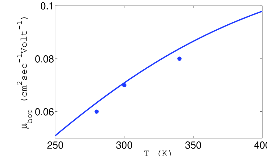
Figure 1: (Color online) Mobility from LL transition in a-Si (T$>$ 250K): solid line is computed from Eq.(85) with parameters: $\lambda_{LL}=0.2eV,~{}\Delta G_{LL}=0.05eV,~{}J_{LL}=0.02eV$. The star symbols are experimental datamo ; tie ; cer ; koc .

Even at moderately high temperature $k_{B}T\gtrsim\hbar\overline{\omega}$, the contribution from diagonal transition, i.e. 1 in last square bracket can be neglected. The main contribution of the ‘time’ integral comes fromHol2 the neighborhood of $\tau=0$. Expand $\cos\tau\omega_{\alpha}\thickapprox 1-\tau^{2}\omega_{\alpha}^{2}/2$ and effect the Gaussian integral, Eq.(82) is changed into

$$W_{T}(A_{1}\rightarrow A_{3})=\frac{J_{A_{3}A_{1}}^{2}}{\hbar^{2}}\exp\{\frac{-\beta}{2}[(E_{A_{3}}^{0}+\mathcal{E}_{b}^{A_{3}})-(E_{A_{1}}^{0}+\mathcal{E}_{b}^{A_{1}})]\}$$ (83)

$$\exp\{-\frac{1}{2}\sum_{\alpha}(\theta_{\alpha}^{A_{3}}-\theta_{\alpha}^{A_{1}})^{2}\tanh\frac{{}^{\beta\hbar\omega_{\alpha}}}{4}\}$$

$$(2\pi)^{1/2}[\frac{1}{2}\sum_{\alpha}(\theta_{\alpha}^{A_{3}}-\theta_{\alpha}^{A_{1}})^{2}\omega_{\alpha}^{2}\text{csch}\frac{\beta\hbar\omega_{\alpha}}{2}]^{-1/2}\exp(-\frac{[(E_{A_{3}}^{0}+\mathcal{E}_{b}^{A_{3}})-(E_{A_{1}}^{0}+\mathcal{E}_{b}^{A_{1}})]^{2}}{\sum_{\alpha}(\theta_{\alpha}^{A_{3}}-\theta_{\alpha}^{A_{1}})^{2}\hbar^{2}\omega_{\alpha}^{2}\text{csch}\frac{\beta\hbar\omega_{\alpha}}{2}})$$

It can be viewed as a generalization of Holstein’s result for small polaron hopping (cf. Eq.(77) of ref.Hol2 ) to the transition between two localized states. The transfer integral $J_{A_{3}A_{1}}\varpropto e^{-qR_{31}}$, $q$ is some constant. In the electric conduction, only the jumps between the nearest localized states are important. The dc conductivity from the localized electrons isrei

$$\sigma_{\text{dc}}^{LL}=\mu_{\text{hop}}^{LL}N_{L}c(1-c)e,\text{ \ \ }\mu_{\text{hop}}^{LL}=\frac{eR_{31}^{2}}{k_{B}T}W_{T}$$ (84)

where $n_{L}$ is the number of electrons in the localized states, $c=n_{L}/N_{L}$. Eq.(84) was derived from the Kubo formula for optical-phonon-assisted hoppingEmin75 .

At ‘very’ high temperature $k_{B}T\gtrsim 2.5\hbar\overline{\omega}$, one can use $\tanh x\thickapprox x$ and csch$x\thickapprox\frac{1}{x}$ (the error is less than $0.003$ when $x<0.2$). Eq.(83) is changed into

$$W_{T}(A_{1}\rightarrow A_{3})=\nu_{LL}e^{-E_{a}^{LL}/k_{B}T},\text{ \ }\nu_{LL}=\frac{J_{A_{3}A_{1}}^{2}}{\hbar}[\frac{\pi}{\lambda_{LL}k_{B}T}]^{1/2}\text{,\ \ }E_{a}^{LL}=\frac{\lambda_{LL}}{4}(1+\frac{\Delta G_{LL}^{0}}{\lambda_{LL}})^{2}$$ (85)

where

$$\Delta G_{LL}^{0}=(E_{A_{3}}^{0}+\mathcal{E}_{b}^{A_{3}})-(E_{A_{1}}^{0}+\mathcal{E}_{b}^{A_{1}}),\text{ \ }\lambda_{LL}=\frac{1}{2}\sum_{\alpha}M_{\alpha}\omega_{\alpha}^{2}(\Theta_{\alpha}^{A_{3}}-\Theta_{\alpha}^{A_{1}})^{2}$$ (86)

$\Delta G_{LL}^{0}$ is the energy difference between two localized states. $\lambda_{LL}$ is the reorganization energy which depends on the vibrational configurations $\{\Theta_{\alpha}^{A_{3}}\}$ and $\{\Theta_{\alpha}^{A_{1}}\}$ of the two localized states. Because $\Theta_{\alpha}^{A}$ does not have determined sign for different state and mode, one can only roughly estimate $\lambda_{LL}\thicksim k^{-1}(\frac{Z^{\ast}e^{2}}{4\pi\epsilon_{0}\xi^{2}})^{2}$. $E_{a}^{LL}$ is about several tens meV. It is in agreement with observed value of a-Si. According to Eqs.(40), (39) and (60), if two localized states are in two different spatial regions, then the atoms displaced by e-ph interaction are different for two states. $\lambda_{LL}$ can not be zero. If the spatial regions for two localized states have overlap, there is possibility that some atoms are moved in similar way in two states by e-ph interaction, $\lambda_{LL}$ could be small. $\lambda_{LL}$ is zero for two extended states, because for extended states the static displacements of the atoms are zero. Molecular dynamics gives phonon spectrum and the eigenvector $\Delta_{p_{A_{1}}\alpha}$ of each mode, and therefore the reorganization energy $\lambda_{LL}$. Eq.(85) is the transition probability between two localized states in an amorphous solid, it has the same form as Eq.(1).

Fig.1 is the temperature dependence of mobility of a-Si for T$>250$K($\thickapprox$0.02eV), plotted from Eqs.(84) and (85) according to a group of typical parameters: $R_{A_{3}A_{1}}=5$Å, $\lambda_{LL}$

$=0.2$eV, $\Delta G_{LL}=0.05$eV (about one half mobility edge) and $J_{A_{3}A_{1}}=0.02$eV. Using above parameters, $W_{T}\thicksim 10^{12}$sec^-1. The computed mobility agrees with the measurementsmo ; tie ; cer ; koc .

III.3 Low temperatures

At low temperature, the probability of diagonal transition and the probability of non-diagonal transition is comparable. The probability of diagonal transition is given by

$$W_{T}^{(d)}(A_{1}\cdots N_{\alpha}\cdots\rightarrow A_{3}\cdots N_{\alpha}\cdots)=\frac{2\pi}{\hbar}J_{A_{3}A_{1}}^{2}\delta[(E_{A_{3}}^{0}+\mathcal{E}_{b}^{A_{3}})-(E_{A_{1}}^{0}+\mathcal{E}_{b}^{A_{1}})]$$ (87)

$$\exp\{-\sum_{\alpha}(N_{\alpha}+\frac{1}{2})(\theta_{\alpha}^{A_{3}}-\theta_{\alpha}^{A_{1}})^{2}\}$$

in the same approximation as Eq.(76). The first line is the expression for the transition between two electronic states without the phonon environment. The last exponential factor of Eq.(87) also appears in the corresponding expression for non-diagonal transition. It can be explained as the decrease of transfer integral caused by electron-vibration coupling.

At zero temperature $N_{\alpha}=0$, and only zero point vibration remains. The transition between two localized states is then pure quantum tunneling. At finite temperature, one needs to average Eq.(87) over the equilibrium phonon distribution:

$$W_{T}^{(d)}(A_{1}\rightarrow A_{3})=\frac{2\pi}{\hbar}J_{A_{3}A_{1}}^{2}\delta[(E^{A_{1}}+\mathcal{E}_{b}^{A_{1}})-(E^{A_{3}}+\mathcal{E}_{b}^{A_{3}})]$$ (88)

$$\exp\{-\frac{1}{2}\sum_{\alpha}(\theta_{\alpha}^{A_{3}}-\theta_{\alpha}^{A_{1}})^{2}\coth\frac{\beta\hbar\omega_{\alpha}}{2}\}$$

The lower value of diagonal transition probability in non-zero temperature comparing with that of zero temperature may be understood as that thermal vibrations disturb quantum tunneling. Group the exponential function and $J_{A_{3}A_{1}}^{2}$ in Eq.(88) together, one may say that transfer integral is reduced in a multi-phonon process. This is similar to that the effective band width decreases with e-ph coupling which was derived from a different modelcap1 ; fei .

.

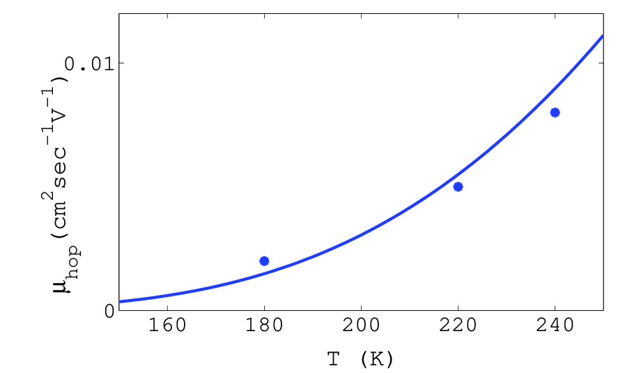
Figure 2: (Color online) Mobility from LL transition in a-Si (T$<$ 250K): solid line is computed from Eq.(90) with parameters: $\Delta G_{LL}=0.05eV,~{}J_{LL}=0.02eV,~{}\bar{\omega}=2\pi\times 850$cm^-1. The star symbols are experimental datamo .

In low temperature $k_{B}T\lesssim\hbar\overline{\omega}/10$ (csch$x<0.0135$ when $x>5$), the exponent in the last exponential of Eq.(82) is small. The exponential can be expanded in Taylor series of its exponent, then the ‘time’ integral can be finished. Denote

$$f(\omega_{\alpha})=\frac{1}{2}(\theta_{\alpha}^{A_{3}}-\theta_{\alpha}^{A_{1}})^{2}\text{csch}\frac{\beta\hbar\omega_{\alpha}}{2}$$ (89)

the result is

$$W_{T}(A_{1}\rightarrow A_{3})=\frac{2\pi J_{A_{3}A_{1}}^{2}}{\hbar}\exp\{\frac{-\beta\Delta G_{LL}^{0}}{2}\}\exp\{-\frac{1}{2}\sum_{\alpha}(\theta_{\alpha}^{A_{3}}-\theta_{\alpha}^{A_{1}})^{2}\coth\frac{{}^{\beta\hbar\omega_{\alpha}}}{2}\}$$ (90)

$$\{\sum_{\alpha}f(\omega_{\alpha})\frac{1}{2}[\delta(\Delta G_{LL}^{0}+\hbar\omega_{\alpha})+\delta(\Delta G_{LL}^{0}-\hbar\omega_{\alpha})]$$

$$+\sum_{\alpha\alpha^{\prime}}f(\omega_{\alpha})f(\omega_{\alpha^{\prime}})\frac{1}{8}[\delta(\Delta G_{LL}^{0}+\hbar\omega_{\alpha}+\hbar\omega_{\alpha^{\prime}})+\delta(\Delta G_{LL}^{0}-\hbar\omega_{\alpha}-\hbar\omega_{\alpha^{\prime}})$$

$$+\delta(\Delta G_{LL}^{0}+\hbar\omega_{\alpha}-\hbar\omega_{\alpha^{\prime}})+\delta(\Delta G_{LL}^{0}-\hbar\omega_{\alpha}+\hbar\omega_{\alpha^{\prime}})]$$

$$+\cdots\}$$

In fact $\coth\frac{{}^{\beta\hbar\omega_{\alpha}}}{2}$ in the second exponential factor can be replaced by 1 when $k_{B}T\lesssim\hbar\overline{\omega}/8$ (coth$x-1<0.0007$ when $x>4$). The terms in the curly bracket are single-phonon transition, 2-phonon transition, etc. $f$ quickly decreases with decreasing temperature, only single-phonon processes are important at low temperature. Because low frequency modes have larger density of states in amorphous solids, multi-phonon processes are also visible at low temperature. Fig.2 is the mobility from LL transition at low temperature regime calculated from Eq.(90) with parameters $\Delta G_{LL}=0.05eV,~{}J_{LL}=0.02eV,~{}\bar{\omega}=2\pi\times 850$cm^-1 (taken from ref.col, ). No reorganization is needed at low temperature regime, but function f decreases with temperature rapidly. The separation temperature T=250K in data fittingmo ; cer is higher than the estimated upper limit of low temperature regime $\bar{\omega}/10\sim 122$K.

The activation energy for the transition between two mid-gap states is just the energy difference between the two levels. For mid-gap states, variable range hopping is an effective conduction mechanism at low temeraturemotv ; aps . Eq.(90) is the conduction of tail states at low temperature due to non-diagonal LL transition. The activation energy $\frac{\Delta G_{LL}^{0}}{2}$ is one half the energy difference between two localized states. This is contrast with the high temperature partner Eq.(85) where activation energy involves reorganization energy. Therefore variable range transition is also an effective conduction mechanism for tail states as non-diagonal transition in the low temperature regime ($k_{B}T\lesssim\hbar\overline{\omega}/10$). Thus $\frac{\hbar\overline{\omega}}{10k_{B}}$ is a rough upper limit temperature of variable range  hopping. In a-Si, $\overline{\omega}/10\thicksim 122$K roughly agrees with the upper limit temperaturemd of variable range hopping (100K).

IV transition from a localized state to an extended state

If at the initial moment ($t=0$) the “one electron + many nuclei” system is at state $|A_{1}\cdots N_{\alpha}^{\prime}\cdots\rangle$, then $C^{A_{1}}(\cdots N_{\alpha}^{\prime}\cdots;t=0)=1$ and other coefficients vanish. At later moment $t$, the probability amplitude $F^{B_{2}}(\cdots N_{\alpha}\cdots;t)$ is simply determined by the first order perturbation approximation of Eq.(70):

$$i\hbar\frac{\partial F_{\{N_{\alpha}\}}^{B_{2}}}{\partial t}=\langle B_{2}\cdots N_{\alpha}\cdots|V_{LE}^{tr}|A_{1}\cdots N_{\alpha}^{\prime}\cdots\rangle C_{\{N_{\alpha}^{\prime}\}}^{A_{1}}e^{it(\mathcal{E}_{B_{2}}^{\{N_{\alpha}\}}-\mathcal{E}_{A_{1}}^{\{N_{\alpha}^{\prime}\}})/\hbar}$$ (91)

It describes the transition from localized state $|A_{1}\cdots N_{\alpha}^{\prime}\cdots\rangle$ to extended state $|B_{2}\cdots N_{\alpha}\cdots\rangle$ caused by the transfer integral $J^{\prime}{}_{B_{2}A_{1}}$. Expand $\Phi_{N_{\alpha}^{\prime}}(\theta_{\alpha}-\theta_{\alpha}^{A_{1}})$ around $\theta_{\alpha}$ to the second order of $\theta_{\alpha}^{A_{1}}$, the integral in matrix element (71) can be effected. Then the transition probability from localized state $A_{1}$ to extended state $B_{2}$ is

$$W_{T}(A_{1}\rightarrow B_{2})=\frac{J^{\prime 2}{}_{B_{2}A_{1}}}{\hbar^{2}}e^{-\beta(E_{B_{2}}-E_{A_{1}}^{0}-\mathcal{E}_{A_{1}}^{b})/2}\exp\{-\frac{1}{2}\sum_{\alpha}(\theta_{\alpha}^{A_{1}})^{2}\coth\frac{\beta\hbar\omega_{\alpha}}{2}\}$$

$$\int_{-t}^{t}d\tau\exp\{\frac{i\tau}{\hbar}(E_{B_{2}}-E_{A_{1}}^{0}-\mathcal{E}_{A_{1}}^{b})\}[\exp\{\frac{1}{2}\sum_{\alpha}(\theta_{\alpha}^{A_{1}})^{2}\text{csch}\frac{\beta\hbar\omega_{\alpha}}{2}\cos\omega_{\alpha}\tau\}-1]$$ (92)

For moderately high temperature $k_{B}T\gtrsim\hbar\overline{\omega}$, the 1 in the last square bracket can be neglected. Expand $\cos\omega_{\alpha}\tau\thickapprox 1-\frac{\tau^{2}\omega_{\alpha}^{2}}{2}$, the integral is a Gaussian integral,

$$W_{T}^{LE}=\frac{J^{\prime 2}{}_{B_{2}A_{1}}}{\hbar^{2}}e^{-\beta(E_{B_{2}}-E_{A_{1}}^{0}-\mathcal{E}_{A_{1}}^{b})/2}\exp\{-\frac{1}{2}\sum_{\alpha}(\theta_{\alpha}^{A_{1}})^{2}\tanh\frac{\beta\hbar\omega_{\alpha}}{4}\}$$

$$(2\pi)^{1/2}[\frac{1}{2}\sum_{\alpha}(\theta_{\alpha}^{A_{1}})^{2}\omega_{\alpha}^{2}\text{csch}\frac{\beta\hbar\omega_{\alpha}}{2}]^{-1/2}\exp(-\frac{[(E_{A_{3}}^{0}+\mathcal{E}_{b}^{A_{3}})-(E_{A_{1}}^{0}+\mathcal{E}_{b}^{A_{1}})]^{2}}{\sum_{\alpha}(\theta_{\alpha}^{A_{1}})^{2}\hbar^{2}\omega_{\alpha}^{2}\text{csch}\frac{\beta\hbar\omega_{\alpha}}{2}})$$ (93)

For ‘very’ high temperature $k_{B}T\gtrsim 2.5\hbar\overline{\omega},$ Eq.(93) is further simplified as:

$$W_{T}^{LE}=\nu_{LE}e^{-E_{a}^{LE}/k_{B}T},\text{ \ \ }E_{a}^{LE}=\frac{\lambda_{LE}}{4}(1+\frac{\Delta G_{LE}^{0}}{\lambda_{LE}})^{2}$$ (94)

where

$$\Delta G_{LE}^{0}=E_{B_{2}}-(E_{A_{1}}^{0}+\mathcal{E}_{A_{1}}^{b})$$ (95)

is the energy difference between extended state $B_{2}$ and localized state $A_{1}$.

$$\nu_{LE}=\frac{J^{\prime 2}{}_{B_{2}A_{1}}}{\hbar}(\frac{\pi}{\lambda_{LE}k_{B}T})^{1/2},\text{ }\lambda_{LE}=\frac{1}{2}\sum_{\alpha}M_{\alpha}\omega_{\alpha}^{2}(\Theta_{\alpha}^{A_{1}})^{2}$$ (96)

$\lambda_{LE}$ is the reorganization energy for transition from localized state $A_{1}$ to extended state $B_{2}$. It is interesting to notice that activation energy $E_{a}^{LE}$ for LE transition can be obtained by assume $\Theta_{\alpha}^{A_{3}}=0$ in $\lambda_{LL}$. Transition from a localized state to an extended state corresponds to that a particle escapes a barrier along reaction pathkram .

From their expressions (86) and (96), we know $\lambda_{LE}$ is same order of magnitude as $\lambda_{LL}$. $\Delta G_{LE}^{0}$ is order of mobility edge, several times larger than $\Delta G_{LL}^{0}$. $J^{\prime}{}_{B_{2}A_{1}}$ is several times larger than $J^{\prime}{}_{A_{3}A_{1}}$. The spatial displacement of the electron in a LE transition is about the linear size of the localized state. In general the LE transition probability is smaller than that of the LL transition. From Eqs.(94) and (85), $W_{T}^{LE}$ becomes comparable with $W_{T}^{LL}$ only when temperature is higher than $k_{B}^{-1}(E_{a}^{LE}-E_{a}^{LL})[2\ln(J_{LE}/J_{LL})]^{-1}$. The mobility edge of a-Si is about 0.1eV, therefore LL transition is dominant in intrinsic a-Si below 580K. However if higher localized states close to the mobility edge are occupied due to doping, there exist some extended states which satisfy $\Delta G_{LE}^{0}\thicksim\Delta G_{LL}^{0}$. For these LE transitions, $E_{a}^{LE}$ is comparable to $E_{a}^{LL}$. The LE transition probability is about 10 times larger than that of LL transition. For these higher localized states, using parameters given for LL  transition in a-Si, $W_{T}^{LE}\thicksim 10^{13}$Sec^-1. Comparing Eqs.(84) and (96), from the value of hopping mobility 0.05 cm²Sec^-1V^-1, we expect the mobility from LE transition is several tenths cm²Sec^-1V^-1 for a-Si, the same order of magnitude as observed ‘drift mobility’tie ; cer .

The probability of diagonal transition is given by

$$W_{T}^{(d)}(B_{2}\cdots N_{\alpha}\cdots\rightarrow A_{1}\cdots N_{\alpha}\cdots)=\frac{2\pi}{\hbar}J^{\prime 2}{}_{B_{2}A_{1}}\delta[E_{B_{2}}-(E_{A_{1}}^{0}+\mathcal{E}_{A_{1}}^{b})]$$ (97)

$$\exp\{-\sum_{\alpha}(N_{\alpha}+\frac{1}{2})(\theta_{\alpha}^{A_{1}})^{2}\}$$

The last exponential factor can be explained as the decrease of transition integral caused by electron-vibration coupling. At zero temperature $N_{\alpha}=0$, the transition from a localized state to an extended state is then pure quantum tunneling. At finite temperature, one needs to average Eq.(97) over the equilibrium phonon distribution:

$$W_{T}^{(d)}(A_{1}\rightarrow B_{2})=\frac{2\pi}{\hbar}J^{\prime 2}{}_{B_{2}A_{1}}\exp\{-\frac{1}{2}\sum_{\alpha}(\theta_{\alpha}^{A_{1}})^{2}\coth\frac{\beta\hbar\omega_{\alpha}}{2}\}\delta[E_{B_{2}}-(E_{A_{1}}^{0}+\mathcal{E}_{b}^{A_{1}})]$$ (98)

In low temperature $k_{B}T\lesssim\hbar\overline{\omega}/10$, the exponent in the last exponential of Eq.(92) is small. The exponential can be expanded in Taylor series of its exponent, then the ‘time’ integral can be finished. Denote

$$f_{LE}(\omega_{\alpha})=\frac{1}{2}(\theta_{\alpha}^{A_{1}})^{2}\text{csch}\frac{\beta\hbar\omega_{\alpha}}{2}$$ (99)

the result is

$$W_{T}(A_{1}\rightarrow B_{2})=\frac{2\pi J^{\prime 2}{}_{B_{2}A_{1}}}{\hbar}\exp\{\frac{-\beta\Delta G_{LE}^{0}}{2}\}\exp\{-\frac{1}{2}\sum_{\alpha}(\theta_{\alpha}^{A_{1}})^{2}\coth\frac{{}^{\beta\hbar\omega_{\alpha}}}{2}\}$$ (100)

$$\{\sum_{\alpha}f_{LE}(\omega_{\alpha})\frac{1}{2}[\delta(\Delta G_{LE}^{0}+\hbar\omega_{\alpha})+\delta(\Delta G_{LE}^{0}-\hbar\omega_{\alpha})]$$

$$+\sum_{\alpha\alpha^{\prime}}f_{LE}(\omega_{\alpha})f_{LE}(\omega_{\alpha^{\prime}})\frac{1}{8}[\delta(\Delta G_{LE}^{0}+\hbar\omega_{\alpha}+\hbar\omega_{\alpha^{\prime}})+\delta(\Delta G_{LE}^{0}-\hbar\omega_{\alpha}-\hbar\omega_{\alpha^{\prime}})$$

$$+\delta(\Delta G_{LE}^{0}+\hbar\omega_{\alpha}-\hbar\omega_{\alpha^{\prime}})+\delta(\Delta G_{LE}^{0}-\hbar\omega_{\alpha}+\hbar\omega_{\alpha^{\prime}})]$$

$$+\cdots\}$$

Formally type (2) transition is quite similar to type (1) transition. To obtain the former, one needs to make substitutions: $J{}_{A_{3}A_{1}}\rightarrow J^{\prime}{}_{B_{2}A_{1}}$ $\Theta_{\alpha}^{A_{3}}-\Theta_{\alpha}^{A_{1}}\rightarrow\Theta_{\alpha}^{A_{1}}$ and $[(E^{A_{1}}+\mathcal{E}_{b}^{A_{1}})-(E^{A_{3}}+\mathcal{E}_{b}^{A_{3}})]\rightarrow[E_{B_{2}}-(E_{A_{1}}^{0}+\mathcal{E}_{b}^{A_{1}})]$ in corresponding expressions of the former. However the physical meaning of the two are completely different: they are reflected in the transfer integrals Eqs.(29) and (33).

Consider a localized state and an extended state, both of them are close to the mobility edge. Then $\Delta G_{LE}^{0}$ is small. For such a localized state, the displacements of the atoms induced by the polarization of the localized state (cf. $\Theta_{\alpha}^{A_{1}}$ in Eq.(59)) are small. Its atomic configuration is similar to that of an extended state. Therefore the reorganization energy $\lambda_{LE}$ is small. The transition probability (94) can be large. Similar picture has been suggested long time ago in name of phonon-induced delocalizationkik . The inelastic process makes the concept of localization meaninglessthou ; im for the states close to the mobility edge.

V transition from an extended state to a localized state

If at the initial moment the electron+nuclei system is at state $|B_{1}\cdots N_{\alpha}^{\prime}\cdots\rangle$, then $F^{B_{1}}(\cdots N_{\alpha}^{\prime}\cdots;t=0)=1$ and other coefficients are zero. At later moment $t$, probability amplitude $C^{A_{2}}(\cdots N_{\alpha}\cdots;t)$ is determined by first order perturbation theory from Eq.(67):

$$i\hbar\frac{\partial C^{A_{2}}}{\partial t}=\langle A_{2}\cdots N_{\alpha}\cdots|V_{EL}^{e-ph}|B_{1}\cdots N_{\alpha}^{\prime}\cdots\rangle F^{B_{1}}(\cdots N_{\alpha}^{\prime}\cdots;t)e^{it(\mathcal{E}_{A_{2}}^{\{N_{\alpha}\}}-\mathcal{E}_{B_{1}}^{\{N_{\alpha}^{\prime}\}})/\hbar}$$ (101)

Expand $\Phi_{N_{\alpha}}(\theta_{\alpha}-\theta_{\alpha}^{A_{2}})$ around $\theta_{\alpha}$ to second order of $\theta_{\alpha}^{A_{2}}$, effect the multiple integral over normal modes, the matrix element (69) can be calculated. The diagonal transition probability (in which the phonon state invariant before and after the change in electronic state) induced by electron-phonon interaction is

$$W_{T}^{(d)}(B_{1}\rightarrow A_{2})=\delta(E_{A_{2}}^{0}+\mathcal{E}_{A_{2}}^{b}-E_{B_{1}})\frac{2\pi}{\hbar}\exp\{-\frac{1}{2}\sum_{\alpha}(\theta_{\alpha}^{A_{2}})^{2}\coth\frac{\beta\hbar\omega_{\alpha}}{2}\}\frac{1}{4}\sum_{\alpha^{\prime}}(K_{A_{2}B_{1}}^{\prime\alpha}\Theta_{\alpha^{\prime}}^{A_{2}})^{2}$$ (102)

The probability of the transition from extended state $|B_{1}\rangle$ to localized state $|A_{2}\rangle$ is

$$W_{T}(B_{1}\rightarrow A_{2})=\frac{1}{\hbar^{2}}\exp\{-\frac{\beta}{2}(E_{A_{2}}^{0}+\mathcal{E}_{A_{2}}^{b}-E_{B_{1}})\}\exp\{-\frac{1}{2}\sum_{\alpha}(\theta_{\alpha}^{A_{2}})^{2}\coth\frac{\beta\hbar\omega_{\alpha}}{2}\}(I_{1}+I_{2})$$ (103)

where

$$I_{1}=\int_{-t}^{t}d\tau\exp\{\frac{i\tau}{\hbar}(E_{A_{2}}^{0}+\mathcal{E}_{A_{2}}^{b}-E_{B_{1}})\}\exp\{\frac{1}{2}\sum_{\alpha}(\theta_{\alpha}^{A_{2}})^{2}\text{csch}\frac{\beta\hbar\omega_{\alpha}}{2}\cos\omega_{\alpha}\tau\}$$ (104)

$$[\sum_{\alpha^{\prime}}(\frac{1}{2}(K_{A_{2}B_{1}}^{\prime\alpha^{\prime}})^{2}+\frac{1}{4}(K_{A_{2}B_{1}}^{\prime\alpha^{\prime}}\theta_{\alpha^{\prime}}^{A_{2}})^{2}\coth\frac{\beta\hbar\omega_{\alpha^{\prime}}}{2})\frac{\hbar}{M_{\alpha^{\prime}}\omega_{\alpha^{\prime}}}\text{csch}\frac{\beta\hbar\omega_{\alpha^{\prime}}}{2}\cos\omega_{\alpha^{\prime}}\tau$$

$$-\frac{1}{4}\sum_{\alpha^{\prime}}\frac{\hbar}{M_{\alpha^{\prime}}\omega_{\alpha^{\prime}}}(K_{A_{2}B_{1}}^{\prime\alpha^{\prime}}\theta_{\alpha^{\prime}}^{A_{2}})^{2}\text{csch}^{2}\frac{\beta\hbar\omega_{\alpha^{\prime}}}{2}\cos^{2}\omega_{\alpha^{\prime}}\tau]$$

and

$$I_{2}=[\frac{1}{4}\sum_{\alpha^{\prime}}(K_{A_{2}B_{1}}^{\prime\alpha}\Theta_{\alpha^{\prime}}^{A_{2}})^{2}]\int_{-t}^{t}d\tau\exp\{\frac{i\tau}{\hbar}(E_{A_{2}}^{0}+\mathcal{E}_{A_{2}}^{b}-E_{B_{1}})\}[\exp\{\frac{1}{2}\sum_{\alpha}(\theta_{\alpha}^{A_{2}})^{2}\text{csch}\frac{\beta\hbar\omega_{\alpha}}{2}\cos\omega_{\alpha}\tau\}-1]$$ (105)

At moderately high temperature $k_{B}T\gtrsim\hbar\overline{\omega}$, by expanding $\cos x\thickapprox 1-\frac{x^{2}}{2}$, the integrals $I_{1}$ and $I_{2}$ can be carried out. One has

$$W_{T}^{EL}(B_{1}\rightarrow A_{2})=\frac{1}{\hbar^{2}}\exp\{-\frac{\beta}{2}(E_{A_{2}}^{0}+\mathcal{E}_{A_{2}}^{b}-E_{B_{1}})\}\exp\{-\frac{1}{2}\sum_{\alpha}(\theta_{\alpha}^{A_{2}})^{2}\tanh\frac{\beta\hbar\omega_{\alpha}}{4}\}$$ (106)

$$(2\pi)^{1/2}[\frac{1}{2}\sum_{\alpha}(\theta_{\alpha}^{A_{2}})^{2}\omega_{\alpha}^{2}\text{csch}\frac{\beta\hbar\omega_{\alpha}}{2}]^{-1/2}\exp(-\frac{(E_{A_{2}}^{0}+\mathcal{E}_{A_{2}}^{b}-E_{B_{1}})^{2}}{\sum_{\alpha}(\theta_{\alpha}^{A_{2}})^{2}\hbar^{2}\omega_{\alpha}^{2}\text{csch}\frac{\beta\hbar\omega_{\alpha}}{2}})$$

$$\{\frac{1}{4}\sum_{\alpha^{\prime}}(K_{A_{2}B_{1}}^{\prime\alpha}\Theta_{\alpha^{\prime}}^{A_{2}})^{2}+\sum_{\alpha^{\prime}}[\frac{(K_{A_{2}B_{1}}^{\prime\alpha})^{2}\hbar}{2M_{\alpha^{\prime}}\omega_{\alpha^{\prime}}}\text{csch}\frac{\beta\hbar\omega_{\alpha^{\prime}}}{2}+\frac{(K_{A_{2}B_{1}}^{\prime\alpha}\Theta_{\alpha^{\prime}}^{A_{2}})^{2}}{8}\text{sech}^{2}\frac{\beta\hbar\omega_{\alpha^{\prime}}}{4}]$$

$$-[2(\sum_{\alpha}\omega_{\alpha}^{2}(\theta_{\alpha}^{A_{2}})^{2}\text{csch}\frac{\beta\hbar\omega_{\alpha}}{2})^{-1}-4\frac{(E_{A_{2}}^{0}+\mathcal{E}_{A_{2}}^{b}-E_{B_{1}})^{2}}{(\sum_{\alpha}\hbar\omega_{\alpha}^{2}(\theta_{\alpha}^{A_{2}})^{2}\text{csch}\frac{\beta\hbar\omega_{\alpha}}{2})^{2}}]$$

$$\times\sum_{\alpha^{\prime}}[\frac{(K_{A_{2}B_{1}}^{\prime\alpha})^{2}\hbar\omega_{\alpha^{\prime}}}{4M_{\alpha^{\prime}}}\text{csch}\frac{\beta\hbar\omega_{\alpha^{\prime}}}{2}+\frac{\omega_{\alpha^{\prime}}^{2}}{8}(K_{A_{2}B_{1}}^{\prime\alpha}\Theta_{\alpha^{\prime}}^{A_{2}})^{2}\coth\frac{\beta\hbar\omega_{\alpha^{\prime}}}{2}\text{csch}\frac{\beta\hbar\omega_{\alpha^{\prime}}}{2}-\frac{\omega_{\alpha^{\prime}}^{2}(K_{A_{2}B_{1}}^{\prime\alpha}\Theta_{\alpha^{\prime}}^{A_{2}})^{2}}{4}\text{csch}^{2}\frac{\beta\hbar\omega_{\alpha}}{2}]\}$$

It is interesting to notice that the first two lines of Eq.(106) have the same structure as Eq.(83) and Eq.(93). The non-radiative lifetime of an electron in an extended state is defined as $t_{\text{life}}=1/\sum_{A_{2}}W_{T}^{EL}$.

For very high temperature $k_{B}T\gtrsim 2.5\hbar\overline{\omega}$, Eq.(106) becomes

$$W_{EL}=\nu_{EL}e^{-E_{a}^{EL}/k_{B}T}$$ (107)

with

$$\nu_{EL}=\frac{1}{\hbar}(\frac{\pi}{k_{B}T\lambda_{EL}})^{1/2}\{\frac{1}{4}\sum_{\alpha^{\prime}}(K_{A_{2}B_{1}}^{\prime\alpha^{\prime}}\Theta_{\alpha^{\prime}}^{A_{2}})^{2}+\sum_{\alpha^{\prime}}[\frac{(K_{A_{2}B_{1}}^{\prime\alpha^{\prime}})^{2}\hbar}{2M_{\alpha^{\prime}}\omega_{\alpha^{\prime}}}\text{csch}\frac{\beta\hbar\omega_{\alpha^{\prime}}}{2}+\frac{(K_{A_{2}B_{1}}^{\prime\alpha}\Theta_{\alpha^{\prime}}^{A_{2}})^{2}}{8}\text{sech}^{2}\frac{\beta\hbar\omega_{\alpha^{\prime}}}{4}]$$ (108)

$$-[2(\sum_{\alpha}\omega_{\alpha}^{2}(\theta_{\alpha}^{A_{2}})^{2}\text{csch}\frac{\beta\hbar\omega_{\alpha}}{2})^{-1}-4\frac{(E_{A_{2}}^{0}+\mathcal{E}_{A_{2}}^{b}-E_{B_{1}})^{2}}{(\sum_{\alpha}\hbar\omega_{\alpha}^{2}(\theta_{\alpha}^{A_{2}})^{2}\text{csch}\frac{\beta\hbar\omega_{\alpha}}{2})^{2}}]\times$$

$$\times\sum_{\alpha^{\prime}}[\frac{(K_{A_{2}B_{1}}^{\prime\alpha^{\prime}})^{2}\hbar\omega_{\alpha^{\prime}}}{4M_{\alpha^{\prime}}}\text{csch}\frac{\beta\hbar\omega_{\alpha^{\prime}}}{2}+\frac{\omega_{\alpha^{\prime}}^{2}(K_{A_{2}B_{1}}^{\prime\alpha^{\prime}}\Theta_{\alpha^{\prime}}^{A_{2}})^{2}\coth\frac{\beta\hbar\omega_{\alpha^{\prime}}}{2}}{8}\text{csch}\frac{\beta\hbar\omega_{\alpha^{\prime}}}{2}-\frac{\omega_{\alpha^{\prime}}^{2}(K_{A_{2}B_{1}}^{\prime\alpha^{\prime}}\Theta_{\alpha^{\prime}}^{A_{2}})^{2}}{4}\text{csch}^{2}\frac{\beta\hbar\omega_{\alpha^{\prime}}}{2}]\}$$

and

$$E_{a}^{EL}=\frac{\lambda_{EL}}{4}(1+\frac{\Delta G_{EL}^{0}}{\lambda_{EL}})^{2},\text{ \ \ }\lambda_{EL}=\frac{1}{2}\sum_{\alpha}M_{\alpha}\omega_{\alpha}^{2}(\Theta_{\alpha}^{A_{2}})^{2},\text{\ \ \ }\Delta G_{EL}^{0}=E_{A_{2}}^{0}+\mathcal{E}_{A_{2}}^{b}-E_{B_{1}}<0$$ (109)

$\lambda_{EL}$ is the same order of magnitude as $\lambda_{LL}$. $\Delta G_{EL}^{0}<0$, $E_{a}^{EL}$ is smaller than $E_{a}^{LL}$. $K_{A_{2}B_{1}}^{\prime\alpha^{\prime}}\Theta_{\alpha^{\prime}}^{A_{2}}$ is the same order magnitude as $J_{A_{3}A_{1}}$, EL transition probability is larger than that of LL transition. With the parameters for LL  transition in a-Si, $W_{T}^{EL}\thicksim 10^{13}-10^{14}$sec^-1. In a-Si:H, it leads to a mobility about several tenths of cm²sec^-1V^-1, a value between the observed ‘hopping mobility’ and ‘drift mobility’cer ; koc . However the population in extended states is meaningful only when temperature is high enough or doping is heavy enough. For intrinsic semiconductor, EL transition is not important for conduction at not too high temperature.

$\Delta G_{EL}^{0}<0$ has a deep consequence. From the expression (62) for $\mathcal{E}_{A_{2}}^{b}$ and the order of magnitude of mobility edgesca , the energy difference $\Delta G_{EL}^{0}<0$ is order of several tenths eV. For the extended states with $|\Delta G_{EL}^{0}|/\lambda_{EL}<1$, we are in normal regime: the higher energy of an extended state (i.e. $\frac{\Delta G_{EL}^{0}}{\lambda_{EL}}$ more negative but still $|\Delta G_{EL}^{0}|/\lambda_{EL}<1$), the smaller the activation energy $E_{a}^{EL}$. The higher extended state has shorter lifetime ($0<|\Delta G_{EL}^{0}|/k_{B}T<5$ cf. Fig.3, one takes $\lambda_{EL}/k_{B}T=5$), the electron has less time moves in extended state, it will contribute less to electric conductivity. For extended states with energies far above the mobility edge (such that $|\Delta G_{EL}^{0}|/\lambda_{EL}>1$), we are in Marcus inverted regime ($|\Delta G_{EL}^{0}|/k_{B}T>5$ cf. Fig.3): the higher the energy of an extended state, the larger the activation energy. The higher extended states have long lifetime (as usual experience: the higher energy of the initial state, the faster of the decay), and they will contribute conductivity more. In the middle of the two regimes, $\frac{\Delta G_{EL}^{0}}{\lambda_{EL}}\thickapprox-1$. For these extended states, no activation energy is needed for the transition to localized state. They will quickly decay to the localized states. Reflected in photoluminescence, the luminescence insisting time as a function of luminescence frequency decreases with frequency. In a crystal, phonon assisted non-radiative transition is slowed down by the energy-momentum conservation law, the lifetime of an excited state is long. This phenomenon was found some times ago: in c-Si/SiO2 quantum well structure, the photoluminescence lifetime is about 1ms, the photoluminescence life time is not sensitive to the monitored wavelengthoka . Comparing with crystalline quantum well, the photoluminescence lifetime of a-Si/SiO₂ structure becomes shorter with a decrease in monitored wavelengthkan 13ns at 550nm and 143ns at 750nm. The trend is consisten with the left half part of Fig.3.

.

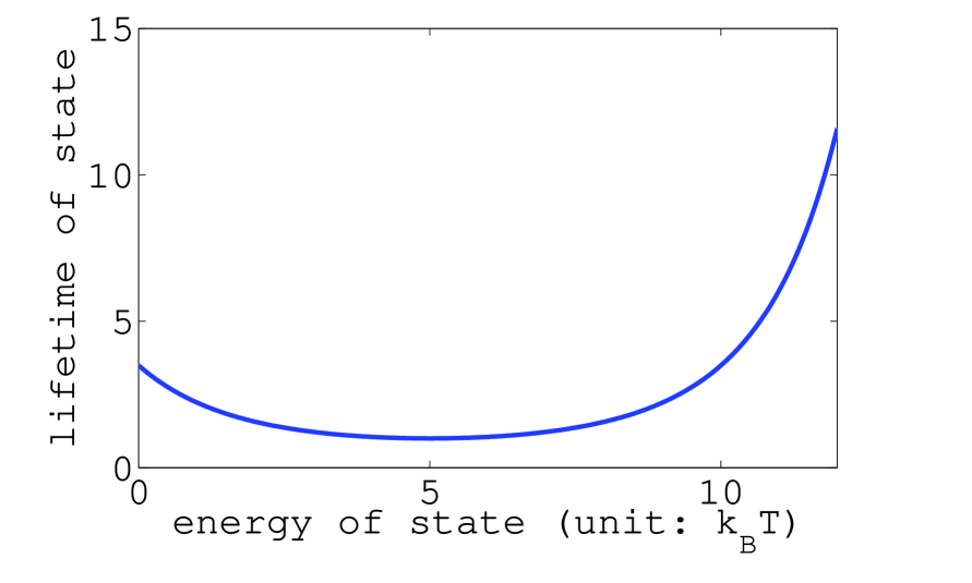
Figure 3: (Color online) Schematic illustration of lifetimes of states as function of energy: energy unit is k${}_{B}T$. $\lambda=5$, E_L is taken as energy zero, the vertical axis is the relative lifetimes of states relative to the shortest one. Marcus inverted region: $E>8$, lifetime increases with energy. The short lifetime belt exists in $3<E<8$. The vertical axis is scaled by $\nu_{EL}$

The preceding discussion is also applicable to the transitions from the extended states in conduction band to the unoccupied localized states in valence band.

At low temperature $k_{B}T\lesssim\hbar\overline{\omega}/10$, one can expand the exponentials in Eqs.(104) and (105) into power series. Then the integrals can be carried out term by term. To 2-phonon processes, the transition probability from extended state $|B_{1}\rangle$ to localized state $|A_{2}\rangle$ is

$$W_{T}(B_{1}\rightarrow A_{2})=\frac{2\pi}{\hbar}\exp\{-\frac{\beta}{2}(E_{A_{2}}^{0}+\mathcal{E}_{A_{2}}^{b}-E_{B_{1}})\}\exp[-\frac{1}{2}\sum_{\alpha}(\theta_{\alpha}^{A_{2}})^{2}\coth\frac{\beta\hbar\omega_{\alpha}}{2}]$$ (110)

$$\{\frac{1}{2}\sum_{\alpha^{\prime}}[\frac{(K_{A_{2}B_{1}}^{\prime\alpha})^{2}\hbar}{2M_{\alpha^{\prime}}\omega_{\alpha^{\prime}}}+\frac{(K_{A_{2}B_{1}}^{\prime\alpha}\Theta_{\alpha^{\prime}}^{A_{2}})^{2}}{4}\coth\frac{\beta\hbar\omega_{\alpha^{\prime}}}{2}]\text{csch}\frac{\beta\hbar\omega_{\alpha^{\prime}}}{2}$$

$$\times[\delta(E_{A_{2}}^{0}+\mathcal{E}_{A_{2}}^{b}-E_{B_{1}}+\hbar\omega_{\alpha^{\prime}})+\delta(E_{A_{2}}^{0}+\mathcal{E}_{A_{2}}^{b}-E_{B_{1}}-\hbar\omega_{\alpha^{\prime}})]$$

$$+\sum_{\alpha^{\prime}}\frac{(K_{A_{2}B_{1}}^{\prime\alpha}\Theta_{\alpha^{\prime}}^{A_{2}})^{2}}{8}(1-\text{csch}^{2}\frac{\beta\hbar\omega_{\alpha^{\prime}}}{2})\sum_{\alpha^{\prime\prime}}f_{EL}(\omega_{\alpha^{\prime\prime}})[\delta(E_{A_{2}}^{0}+\mathcal{E}_{A_{2}}^{b}-E_{B_{1}}+\hbar\omega_{\alpha^{\prime\prime}})+\delta(E_{A_{2}}^{0}+\mathcal{E}_{A_{2}}^{b}-E_{B_{1}}-\hbar\omega_{\alpha^{\prime\prime}})]$$

$$+\frac{1}{4}\sum_{\alpha^{\prime}\alpha^{\prime\prime}}[\frac{(K_{A_{2}B_{1}}^{\prime\alpha})^{2}\hbar}{2M_{\alpha^{\prime}}\omega_{\alpha^{\prime}}}+\frac{(K_{A_{2}B_{1}}^{\prime\alpha}\Theta_{\alpha^{\prime}}^{A_{2}})^{2}}{4}\coth\frac{\beta\hbar\omega_{\alpha^{\prime}}}{2}]\text{csch}\frac{\beta\hbar\omega_{\alpha^{\prime}}}{2}f_{EL}(\omega_{\alpha^{\prime\prime}})$$

$$\times [\delta(E_{A_{2}}^{0}+\mathcal{E}_{A_{2}}^{b}-E_{B_{1}}+\hbar\omega_{\alpha^{\prime}}+\hbar\omega_{\alpha^{\prime\prime}})+\delta(E_{A_{2}}^{0}+\mathcal{E}_{A_{2}}^{b}-E_{B_{1}}+\hbar\omega_{\alpha^{\prime}}-\hbar\omega_{\alpha^{\prime\prime}})$$

$$+ \delta(E_{A_{2}}^{0}+\mathcal{E}_{A_{2}}^{b}-E_{B_{1}}-\hbar\omega_{\alpha^{\prime}}+\hbar\omega_{\alpha^{\prime\prime}})+\delta(E_{A_{2}}^{0}+\mathcal{E}_{A_{2}}^{b}-E_{B_{1}}-\hbar\omega_{\alpha^{\prime}}-\hbar\omega_{\alpha^{\prime\prime}})]$$

$$+[\sum_{\alpha^{\prime}}\frac{(K_{A_{2}B_{1}}^{\prime\alpha}\Theta_{\alpha^{\prime}}^{A_{2}})^{2}}{64}(2-\text{csch}^{2}\frac{\beta\hbar\omega_{\alpha^{\prime}}}{2})]\sum_{\alpha^{\prime\prime}\alpha^{\prime\prime\prime}}f_{EL}(\omega_{\alpha^{\prime\prime}})f_{EL}(\omega_{\alpha^{\prime\prime\prime}})$$

$$\times[\delta(E_{A_{2}}^{0}+\mathcal{E}_{A_{2}}^{b}-E_{B_{1}}+\hbar\omega_{\alpha^{\prime\prime}}+\hbar\omega_{\alpha^{\prime\prime\prime}})+\delta(E_{A_{2}}^{0}+\mathcal{E}_{A_{2}}^{b}-E_{B_{1}}+\hbar\omega_{\alpha^{\prime\prime}}-\hbar\omega_{\alpha^{\prime\prime\prime}})$$

$$+\delta(E_{A_{2}}^{0}+\mathcal{E}_{A_{2}}^{b}-E_{B_{1}}-\hbar\omega_{\alpha^{\prime\prime}}+\hbar\omega_{\alpha^{\prime\prime\prime}})+\delta(E_{A_{2}}^{0}+\mathcal{E}_{A_{2}}^{b}-E_{B_{1}}-\hbar\omega_{\alpha^{\prime\prime}}-\hbar\omega_{\alpha^{\prime\prime\prime}})]$$

$$-\sum_{\alpha^{\prime}}\frac{(K_{A_{2}B_{1}}^{\prime\alpha}\Theta_{\alpha^{\prime}}^{A_{2}})^{2}}{16}\text{csch}^{2}\frac{\beta\hbar\omega_{\alpha^{\prime}}}{2}[\delta(E_{A_{2}}^{0}+\mathcal{E}_{A_{2}}^{b}-E_{B_{1}}+2\hbar\omega_{\alpha^{\prime}})+\delta(E_{A_{2}}^{0}+\mathcal{E}_{A_{2}}^{b}-E_{B_{1}}-2\hbar\omega_{\alpha^{\prime}})]+\cdots\}$$

where

$$f_{EL}(\omega_{\alpha})=\frac{1}{2}(\theta_{\alpha}^{A_{2}})^{2}\text{csch}\frac{\beta\hbar\omega_{\alpha}}{2}$$ (111)

In conduction band, the energy of any localized state is lower than that of any extended state. Thus zero-phonon process cannot conserve energy and therefore is not possible. Because $\Delta G_{EL}^{0}<0,$ factor $\exp[|\Delta G_{EL}^{0}|/(2k_{B}T)]$ increases with decreasing temperature. On the other hand, other factors in Eq.(110) decrease with lowering temperature. There exists an optimal temperature T_∗, at which transition probability is maximum. In non-equilibrium phenomenon like luminescence,  T_∗ may have some traces.

VI transition between extended states caused by electron-phonon interaction

If in the initial moment the “one electron+ many nuclei” system is at state $|B_{1}\cdots N_{\alpha}^{\prime}\cdots\rangle$, then only $F^{B_{1}}(\cdots N_{\alpha}^{\prime}\cdots;t=0)=1$ and other coefficients are zero. At later moment $t$, probability amplitude $F^{B_{2}}(\cdots N_{\alpha}\cdots;t)$ is determined by the first order perturbation theory based on Eq.(70):

$$i\hbar\frac{\partial F_{\{N_{\alpha}\}}^{B_{2}}}{\partial t}=\langle B_{2}\cdots N_{\alpha}\cdots|V_{EE}^{e-ph}|B_{1}\cdots N_{\alpha}^{\prime}\cdots\rangle F_{\{N_{\alpha}^{\prime}\}}^{B_{1}}e^{it(\mathcal{E}_{B_{2}}^{\{N_{\alpha}\}}-\mathcal{E}_{B_{1}}^{\{N_{\alpha}^{\prime}\}})/\hbar}$$ (112)

The matrix element (72) an be calculated from the recursion relation for $z\Phi_{N}(z)$. The transition probability from extended state $|B_{1}\rangle$ to extended state $|B_{2}\rangle$ is

$$W(B_{1}\rightarrow B_{2})=\frac{2\pi}{\hbar}\sum_{\alpha^{\prime}}(K_{B_{2}B_{1}}^{\alpha^{\prime}})^{2}\frac{\hbar}{M_{\alpha^{\prime}}\omega_{\alpha^{\prime}}}[\frac{\overline{N_{\alpha^{\prime}}^{\prime}}}{2}\delta(E_{B_{2}}-E_{B_{1}}-\hbar\omega_{\alpha^{\prime}})+\frac{\overline{N_{\alpha^{\prime}}^{\prime}}+1}{2}\delta(E_{B_{2}}-E_{B_{1}}+\hbar\omega_{\alpha^{\prime}})]$$ (113)

where $\overline{N_{\alpha^{\prime}}^{\prime}}=(e^{\beta\hbar\omega_{\alpha^{\prime}}}-1)^{-1}$ is the average phonon number in the $\alpha^{\prime}$th mode. In a crystal, Eq.(113) arises from inelastic scattering with phonons. Although in amorphous solids one cannot classify the electronic states and the phonon states with wave vectors, Eq.(113) is similar to its crystalline counterpart of phonon inelastic scattering. The relaxation time $\tau(B_{1})$ of state $|B_{1}\rangle$ can be defined as

$$\frac{1}{\tau(B_{1})}=\sum_{B_{2}}W(B_{1}\rightarrow B_{2})[1-f(B_{2})]$$ (114)

$$\sigma^{EE}=n_{E}e\mu^{EE},\text{ \ \ \ }\mu^{EE}=\frac{e\tau}{m}$$ (115)

where $n_{E}$ is the number of electrons in extended states, $\mu^{EE}$ is the mobility of the electrons in extended states. From the observed valuecer of $\mu_{\text{drift}}=0.61$cm²V^-1Sec^-1 of a-Si, one deduces relaxation time $\tau\thicksim 0.35$fs. Take effective nuclear charge Z^∗ of Si as 4, bond length $b=$2.35Å, the coupling constant will be $K\thicksim\frac{Z^{\ast}e^{2}}{4\pi\epsilon_{0}(b/2)^{2}}\thicksim 9.2\times 10^{-8}$N. $W\thicksim\frac{K^{2}}{\hbar M\omega^{2}}\thicksim 6.7\times 10^{12}$sec^-1. The relaxation time $\tau=W^{-1}\thicksim 0.15$ps. The electron moving in extended states scattered by phonons will give a mobility 3 order of magnitude larger than the observed value of ‘drift mobility’. Therefore the drift of electron in extended states is not responsible for the observed ‘drift mobility’.

VI.1 Four types of transitions and conduction mechanisms

Some features of 4 types of transitions are summarized in TABLE 1. With the basic transition probabilities for four types transitions in Sec.III-Sec.VI, the transport properties could be derived from various master equations (Fokker-Planck equation, Boltzmann equation etc.), we will not further pursue this well-known but complicated procedure and only briefly discuss the conduction mechanisms.

In thermal equilibrium at temperature $T$, the ratio $R$ of the number of electrons in the extended states to the number of electrons in localized states is of order $e^{-F/k_{B}T}$, $F$ is the distance between the lower mobility edge and the bottom of conduction band (for a-Si, $F$ is aboutster $0.2$eV. At T=300K, $R\thicksim 4\times 10^{-4}$). However the mobility for a carrier in extended states is much higher than the mobility in localized states. For the extended states outside the short lifetime belt, the life time $t_{\text{life}}$ of a carrier in one of these states is long enough. Under the influence of external electric field, the carrier drifts in these extended states. Thus at higher temperature, transition from localized states to extended states (LE) will lead to an appreciable contribution to conductivity $\sigma_{dc}^{(2)}=\frac{e^{2}n_{E}}{m}\frac{\tau t_{\text{life}}}{\tau+t_{\text{life}}}$,where $m$ is mass of electron, $n_{E}$ is the number of electrons in extended  states. $\tau\thicksim[W(B_{1}\rightarrow B_{2})]^{-1}$ is the mean free time in the extended states determined by Eq.(113). When $t_{\text{life}}>>\tau$, $\sigma_{dc}^{(2)}$ is reduced to the usual formula $\tau e^{2}n_{E}/m$.

In present perturbation treatment, the total conduction comes from four processes: (1) the hopping among localized states; (2) the hoping from a localized state to an extended state; (3) the hopping from an extended state to a localized state and (4) the drift in extended state scattered by phonon. The carriers are pumped to the extended states by type (2) transition.

Table 1: Some features of 4 types of transitions

transitions	origin	phonons needed	activated	role in conduction	$W_{T}$(sec-1)
L$\rightarrow$L	J	multi	yes	direct	$10^{12}$
L$\rightarrow$E	$J^{{}^{\prime}}$	multi	yes	direct+indirect	$10^{10}-10^{13}$
E$\rightarrow$L	$K^{{}^{\prime}}$	multi	yes	direct+indirect	$10^{13}-10^{14}$
E$\rightarrow$E	$K$	single	no	reduce	$10^{13}$

The last column gives the order of magnitude of the transition probability estimated for a-Si at T=300K. The value of LL transition is for the transition between two nearest neighbors. For an intrinsic or a lightly n-doped semiconductor at not too high temperature (T$<$580K for a-Si), only the lower part of conduction tail is occupied. $\Delta G_{LE}$ is large, LE transition probability is about two order of magnitude smaller than that of LL transition. For an intrinsic semiconductor at higher temperature or a doped material, $\Delta G_{LE}^{0}$ becomes comparable with $\Delta G_{LL}^{0}$, LE transition probability is about ten times larger than that of LL transition. The first three types of transitions increase the mobility of an electron, whereas type (4) transition decreases mobility of an electron. Although a stricter solution of Eq.(14) could be obtained by considering the change in the functional form of vibrational states by the motion of the electrons and the change in electronic wave function in the same time. However for a localized state in amorphous semiconductor, the time spent from one localized state to another (10^-10m/10⁵m$\cdot$sec${}^{-1}\thicksim 10^{-16}-10^{-15}$sec) is much shorter than the stay time on one localized state ($10^{-12}$sec). In addition the slow multi-phonon reorganization process of a configuration reduces the impulse of an electron on the network when the electron moves. Thus one can neglect the recoil of lattice by moving an electron. This differs from an ionic crystal where the deformation of the lattice closely stalks the motion of the slow electron.

VI.2 Long time and higher order processes

The perturbation treatments of the fundamental processes given in Sec.IV-Sec.VII are only suitable for short times, in which the probability amplitude of the final state is small. Starting from a localized state we only have $L\rightarrow E$ process and $L\rightarrow L$ process. Starting from an extended state, we only have $E\rightarrow L$ process and $E\rightarrow E$ process. For long time period, higher order processes appear. For example $L\rightarrow E\rightarrow L\rightarrow L\rightarrow E\rightarrow L\rightarrow E\rightarrow E\rightarrow L$ etc. Those high order processes are what occur in the amorphous solids. However, the perturbation picture could be used to compute transport properties. In semiconductors, the number of carriers are smaller than the number of avialable states. The motions of the individual carriers can be viewed as independent. On the other hand, for macroscopic sample, each type of states are highly populated if we consider the whole sample. Thus if we concern the collective behavior of all carriers rather than one individual carrier in a long time period, the picture of the four types of transitions works well statistically.

VII Summary

For amorphous solids, following Holstein’s work on small polaron, we established the evolution equations for localized states and extended states in the presence of lattice vibrations (Eqs.(30) and (31)). To simplify the evolution equations, for localized states, we restrict ourselves to the most localized ones. These localized states are attached to the most distorted regions, and are spatially well separated. One can neglect the overlap integral between two of them and the overlap integral between an extended state and one of the most localized states. For any process involving localized states close to mobility edge, the conclusions obtained from the simplified evolution equations (Eqs.(35) and (36)) are only qualitatively correct.

For short times ($t<<\frac{\hbar}{J},$ $\frac{\hbar}{J^{\prime}},$ $\frac{\hbar}{K},$ $\frac{\hbar}{K^{\prime}}$), perturbation theory can be used to solve Eqs.(35) and (36). One obtains the transition probabilities of LL, LE, EL and EE transitions. In high temperature ($k_{B}T\gtrsim\hbar\overline{\omega}$) and low temperature ($k_{B}T<\hbar\overline{\omega}/10$) limits, the ‘time’ integral in transition probabilities of LL, LE and EL transitions can be carried out analytically. The relative errors are less than 10^-3. In amorphous semiconductors (e.g. a-Si), the transfer integrals $J$ and $J^{\prime},$ and the e-ph interactions $K^{\prime}$ and $K$ are sufficiently small such that the perturbation theory is applicable for a meaningful time period. Although in a sample the motion of a single carrier is a long time and high order process. Because conduction is a collective behavior of many carriers, the results of perturbation theory can be used.

The hopping motion of electron along the direction of electric field during LL, LE and EL transitions directly contributes to conductivity. In external electric field, an electron in extended states moves along the direction of electric field. EE transition deviates the direction of drift which is along the direction of field and reduces the transport of charges. LE transition increases the number of electrons in extended states, whereas EL transition decreases the number of electrons in extended states. They also affect conductivity indirectly.

At ‘very’ high temperature ( $k_{B}T\gtrsim 2.5\hbar\overline{\omega}$), the transition probabilities for the transitions of type (1), type (2) and type (3) are reduced to an Eq.(1)-like formula. It is universal for the processes involving localized state.  If a localized state close to the bottom of conduction band, $\Delta G_{LE}-\Delta G_{LL}$ is about the mobility edge, $W^{LE}$ is one or two order of magnitude smaller than $W^{LL}$. If a localized state close to mobility edge, $\Delta G_{LE}\thicksim\Delta G_{LL},$ because $J^{\prime}$ is several times larger than $J,$ $W^{LE}$ could be one order of magnitude larger than $W^{LL}$. The probability of type (3) is one or two order of magnitude larger than that of LL transition. The reason is $\Delta G_{EL}<0$, $E_{a}^{EL}$ is smaller than $E_{a}^{LL}$ while $K^{\prime}\Theta$ is same order of magnitude as $J$. The probability of EE transition is about 10³ times larger than $W^{LL}$ (cf. Table I). Type (4) transition deviates the direction of the drift motion along the direction of electric field and reduces conductivity. This is contrast with LL, LE and EL transition. The relative contribution to conductivity of four types of transition also highly depends on the number of carriers in extended states and the number of carriers in localized states, which are determined by the extent of doping and temperature.

At low temperature ( $k_{B}T<\hbar\overline{\omega}/10$), the non-diagonal transition is still multi-phonon activated process whatever it is LL, LE or EL transition. The activation energy is just half of the energy difference between final state and initial state ($\Delta G_{LL}/2,$ $\Delta G_{LE}/2,$ $\Delta G_{EL}/2$). The reorganization of vibration configuration is not needed, this is similar to the hopping between mid-gap statesmotv ; aps which does not need reorganization of the static displacementsmd . Thus we expect variable range hopping also works for the LL transitions which are transitions between tail states.

In a-Si for both high and low temperature regimes, the computed temperature dependence of mobility of LL transition agrees with the observedmo ; tie ; cer ; koc ‘hopping mobility’. EE transition offers a mobility which is three times larger than the observed drift mobility. However, in an intrinsic or a lightly doped system, the occupation probability of the extended states is small. The observed ‘drift mobility’ may come from LE transition.

There exists a short lifetime belt of the extended states inside conduction band or valence band. These states favor non-radiation transition by emitting several phonons, have smaller contributions to dc conductivity than other extended states. The fact that photoluminescence lifetime in a-Si/SiO₂ decreases with frequency confirms the existence of short lifetime belt in conduction band. The phonon-assisted non-radiation transition dissipates the population of the excited states in amorphous semiconductors.

Some important points are not addressed in this work. The overlap integral between two less localized states which spread in several distorted regions and the overlap integral between one less localized state and an extended state require the wave function of a less localized state which cannot be described by a single exponential decay function. The coherence between states is subtle in Eqs.(56) and (57). The dependence of conduction on the strength of external field also requires including electric field in the zeroth order in the evolution equations. The drag effectcon06 of water on the conduction of solvated DNA is not included in Eq.(14). We wish to discuss them in near future.

VIII Acknowledgements

We thank the Army Research Office for support under MURI W91NF-06-2-0026, and the National Science Foundation for support under grants DMR 0600073 and 0605890. DAD thanks the Leverhulme Trust (UK) and the National Science Foundation for sabbatical support.

References

• (1) N. F. Mott and E. A. Davis, Electronic Processes in Non-crystalline Materials, Clarendon Press, Oxford (1971).
• (2) H. Muller and P. Thomas, Physical Review Letters, 51, 702 (1983).
• (3) H. Overhof and P. Thomas Electronic Transport in Hydrogenated Amorphous Silicon Springer Tracts in Modern Physics No. 114 (Springer, Berlin, 1989).
• (4) R. A. Marcus, Review of Modern Physics, 65, 599 (1993).
• (5) T. Holstein, Annals of Physics, 8, 325 (1959).
• (6) T. Holstein, Annals of Physics, 8, 343 (1959).
• (7) H. G. Reik, in J. T. Devereese (Ed), Polarons in Ionic and Polar Semiconductors, Chapter VII, North-Holland/American Elsevier, Amsterdam (1972).
• (8) D. Emin, Phys. Rev. Lett. 32, 303 (1974).
• (9) D. Emin, Adv. Phys. 24, 305 (1975).
• (10) D. Emin and T. Holstein, Physical Review Letters, 36, 323 (1976).
• (11) E. Gorham-Bergeron and D. Emin, Phys. Rev. B 15, 3667 (1977).
• (12) D. Emin, Phys. Rev. B 43, 11720 (1991).
• (13) D. Emin and M.-N. Bussac, Physical Review B 49, 14290 (1994).
• (14) M. Kikuchi, J. Non-Cryst. Sol. 59/60, 25 (1983).
• (15) J. Dong and D. A. Drabold, Phys. Rev. Lett. 80, 1928 (1998).
• (16) J. J. Ludlam, S. N. Taraskin, S. R. Elliott and D. A. Drabold, J. Phys. Cond. Matter 17, L321 (2005).
• (17) Y. Pan, M. Zhang and D. A. Drabold, J. Non. Cryst. Sol. 354, 3480 (2008).
• (18) M.-L. Zhang and D. A. Drabold, in preparation.
• (19) L. Pauling and E. B. Wilson, Introduction to quantum mechanics, with applications to chemistry, McGraw-Hill, New York, (1935).
• (20) M.-L. Zhang, B. J. Ka and E. Geva, J. Chem. Phys. 125, 044106 (2006).
• (21) J. Ankerhold and H. Lehle, J. Chem. Phys. 120, 1436 (2004).
• (22) H. A.Kramers, Physica 7, 284 (1940).
• (23) D. A. Drabold, P. A. Fedders, S. Klemm and O. F. Sankey, Physical Review Letters, 67, 2179 (1991).
• (24) R. Atta-Fynn, P. Biswas and D. A. Drabold, Phys. Rev. B 69, 245204 (2004).
• (25) T. D. Lee and D. Pines, Physical Review 92, 883 (1953).
• (26) T. D. Lee, F. E. Low and D. Pines, Physical Review 90, 297 (1953).
• (27) S. G. Christov, Physical Review B 26, 6918 (1982).
• (28) R. A. Marcus, Journal of Chemical Physics 24, 979 (1956).
• (29) R. A. Marcus, Journal of Chemical Physics 24, 966 (1956).
• (30) M.-L, Zhang, S.-S. Zhang and E. Pollak, Journal of Chemical Physics, 119, 11864 (2003).
• (31) A. R. Moore, Applied Physics Letters, 31, 762 (1977).
• (32) T. Tiedje, T. D. Moustakas and J. M. Cebulka, Journal De Physique 42, C4-155, (1981).
• (33) K. Cermak and J. Kocka, Czech J Phys B34, 216 (1984).
• (34) J. Kocka, O. Klima, E. Sipek, C. E. Nebel, G. H. Bauer, G. Juska and M. Hoheisel, Physical Review B45, 6593 (1992).
• (35) M. Capone, W. Stephan and M. Grilli, Physical Review B 56, 4484 (1997).
• (36) D. Feinberg, S. Ciuchi and F. De Pasqualle, Int. J. Phys. B 4, 1317 (1990).
• (37) H. Cole and E. Kineke, Phys. Rev. Lett. 1, 360 (1958).
• (38) N. F. Mott, Phil. Mag., 19, 835, (1969).
• (39) N. Apsley and H. P. Huges, Phil. Mag., 30, 963, (1974).
• (40) D. J. Thouless, Phys. Rev. Lett. 39, 1167(1977).
• (41) Y. Imry, Phys. Rev. Lett. 44, 469 (1980).
• (42) M.-L. Zhang, Y. Pan, F. Inam and D. A. Drabold, Phys. Rev. B 78, 195208 (2008).
• (43) S. Okamoto, Y. Kanemitsu, Solid State Communication 103, 573 (1997).
• (44) Y. Kanemitsu, M. Iiboshi and T. Kushida, Journal of Luminescence 87-89, 463-465 (2000).
• (45) S. Völker, Annu. Rev. Phys. Chem. 40, 499-530 (1989).
• (46) F. Stern, Physical Review B 3, 2636 (1971).
• (47) E. M. Conwell and D. M. Basko, J. Phys. Chem. B 110, 23603 (2006).