Black holes, black strings and cosmological constant

Abstract

We present a review of black holes and black string solutions available in the $d$-dimensional Einstein and Einstein-Maxwell model in the presence of a cosmological constant. Due to the cosmological constant, the equations do not admit explicit solutions for generic values of the parameters and numerical methods are necessary to construct the solutions. Several new features of the solutions are discussed, namely their stability and the occurrence of non-uniform black strings which depend non-trivially on the co-dimension. Black string solutions are further constructed for the Einstein-Gauss-Bonnet model. The influence of the Gauss-Bonnet term on the domain of existence of the black strings is discussed in details.

Extended version of a contribution to the 418th WE-Heraeus Seminar, Bremen, 25-29 August 2008.

I Introduction

In the last years, there has been increasing interest in space-times involving more than four dimensions. Particularly, so called brane-world models brane ; rs have gained a lot of interest. These assume the standard model fields to be confined on a 3-brane embedded in a higher dimensional manifold. Consequently, a large number of higher dimensional black holes has been studied in recent years. The first solutions that have been constructed are the hyperspherical generalisations of well-known black holes solutions such as the Schwarzschild and Reissner-Nordström solutions in more than four dimensions tangherlini as well as the higher dimensional Kerr solutions mp . In $d$ dimensions, these solutions have horizon topology $S^{d-2}$.

In contrast to four dimensions, however, black holes with different horizon topologies should be possible in higher dimensions. An example is a 4-dimensional Schwarzschild black hole extended into one extra dimension, a so-called Schwarzschild black string. These solutions have been discussed extensively especially with emphasis put on their stability gl . A second example, which is important due to its implications for uniqueness conjectures for black holes in higher dimensions is the black ring solution in 5 dimensions with horizon topology $S^{2}\times S^{1}$ er .

On the other hand there is mounting observational evidence in the past few years astrocc that the universe is expanding with acceleration. The simplest explanation for this is a positive cosmological constant. From a more theoretical point of view, the Anti–de–Sitter/Conformal Field Theory (AdS/CFT) correspondence Witten:1998qj ; Maldacena:1997re encourages the investigations of the field equations in the presence of a negative cosmological constant. It therefore make sense to investigate the effects of a cosmological constant – either positive or negative – on black objects. The results of this investigation are discussed in this report.

In the first part (Section II) of this report, we discuss rotating black hole solutions of the $d$ dimensional Einstein-Maxwell model (with $d$ odd). The ansatz chosen for the metric and Maxwell fields leads to a set of differential equations. The domain of existence of these solutions is determined in dependence on the horizon radius and on the strength of the magnetic field. Section III is devoted to several aspects of black strings. In the presence of a negative cosmological constant, these solutions can not be given in explicit form, but have to be constructed numerically. In particular, charged and rotating black strings are considered. The stability of AdS black strings is then discussed and it is shown that they become unstable when the length of the extra dimension gets larger than a horizon-dependent critical value. Preliminary results suggesting the existence of non-uniform black strings, depending both on the extra dimension and on the radial variable associated to the internal space-time, are presented. In the last section various properties of black string solutions of the Einstein-Gauss-Bonnet model are presented. The influence of the Gauss-Bonnet interaction on the domain of existence of the black strings is analyzed in detail.

II Black holes with cosmological constant

In this section we consider the Einstein-Maxwell equations in $d$ dimensions and address the construction of charged, rotating black holes. For odd values of $d$, an ansatz can be done which transforms the full equations into a system of ordinary differential equations. Numerical investigation of the solutions is then possible. The domain of existence of these solutions is determined depending on the horizon radius and on the strength of the magnetic field.

II.1 Model and equations

The Einstein-Maxwell Lagrangian with a cosmological constant $\Lambda$ in a $d-$dimensional space-time is given by

$$I=\frac{1}{16\pi G_{d}}\int_{M}~{}d^{d}x\sqrt{-g}(R-2\Lambda-F_{\mu\nu}F^{\mu\nu})$$

$$-\frac{1}{8\pi G_{d}}\int_{\partial M}d^{d-1}x\sqrt{-h}K,$$ (1)

Here, $G_{d}$ denotes the $d-$dimensional Newton constant. The units are chosen in such a way that $G_{d}$ appears as an overall factor. The last term in (II.1) is the Hawking-Gibbons term; it guarantees the variational principle to be well defined but we will not need it in this report. It is convenient to further define an (Anti-)de-Sitter “radius” $\ell$ according to

$$\Lambda=\pm\frac{(d-2)(d-1)}{2\ell^{2}}.$$ (2)

The Einstein-Maxwell equations are obtained from the variation of the action with respect to the metric and the electromagnetic fields.

The ansatz: We consider space-times with odd dimensions, $d=2N+1$, and assume the metric to be of the form

$$ds^{2}= - b(r)dt^{2}+\frac{dr^{2}}{f(r)}+g(r)\sum_{i=1}^{N-1}\left(\prod_{j=0}^{i-1}\cos^{2}\theta_{j}\right)d\theta_{i}^{2}$$

$$+ h(r)\sum_{k=1}^{N}\left(\prod_{l=0}^{k-1}\cos^{2}\theta_{l}\right)\sin^{2}\theta_{k}\left(d\varphi_{k}-w(r)dt\right)^{2}$$

$$+ p(r)\left\{\sum_{k=1}^{N}\left(\prod_{l=0}^{k-1}\cos^{2}\theta_{l}\right)\sin^{2}\theta_{k}d\varphi_{k}^{2}\right.-\left.\left[\sum_{k=1}^{N}\left(\prod_{l=0}^{k-1}\cos^{2}\theta_{l}\right)\sin^{2}\theta_{k}d\varphi_{k}\right]^{2}\right\}\ .$$

This metric possesses $N+1$ Killing vectors $\partial_{\varphi_{k}}$,$\partial_{t}$, out of which $N$ are associated to conserved angular momenta. The most general Maxwell potential consistent with these symmetries turns out to be

$$A_{\mu}dx^{\mu}=V(r)dt+a_{\varphi}(r)\sum_{k=1}^{N}\left(\prod_{l=0}^{k-1}\cos^{2}\theta_{l}\right)\sin^{2}\theta_{k}d\varphi_{k}$$

The form of the metric (II.1) looks cumbersome, however, for $d=5$, it simplifies to

$$ds^{2} = -b(r)dt^{2}+\frac{dr^{2}}{f(r)}+g(r)d\theta^{2}+p(r)(\sin\theta)^{2}(\cos\theta)^{2}(d\varphi_{1}-d\varphi_{2})^{2}\$$

$$+ h(r)[(\sin\theta)^{2}(d\varphi_{1}-w(r)dt)^{2}+(\cos\theta)^{2}(d\varphi_{2}-w(r)dt)^{2}]$$

Inserting the ansatz above into the Einstein-Maxwell equations results in a system of seven non-linear, coupled differential equations provided $p(r)=g(r)-h(r)$. The Maxwell functions $V(r),a_{\phi}(r)$ as well as the metric functions $b(r),f(r),g(r),h(r),w(r)$ are unknown. One of these functions can be fixed arbitrarily, e.g. by choosing the radial coordinate to be of the Schwarzschild type e.g. $g=r^{2}$.

II.2 Explicit Solutions

The set of differential equations under consideration admits a few explicit solutions in some specific limits. We will remind them before discussing the full solutions.
(i) The vacuum black holes are recovered for vanishing Maxwell fields : $V=a_{\varphi}=0$. The metric fields then take the form

$$f(r)=1-\epsilon\frac{r^{2}}{\ell^{2}}-\frac{2M\Xi}{r^{d-3}}+\frac{2Ma^{2}}{r^{d-1}},~{}h(r)=r^{2}(1+\frac{2Ma^{2}}{r^{d-1}})\ \ ,~{}$$

$$w(r)=\frac{2Ma}{r^{d-3}h(r)},~{}~{}g(r)=r^{2},~{}~{}b(r)=\frac{r^{2}f(r)}{h(r)}\ ,$$ (5)

where $M$ and $a$ are two constants related to the solution’s mass and angular momentum and $\Xi\equiv 1+a^{2}/\ell^{2}$. These solutions generalize the Tangherlini tangherlini and Myers-Perry mp solutions to the case of non-vanishing cosmological constant. From now on, we will denote the angular velocity at the event horizon by $\Omega\equiv w(r_{h})$.

(ii) The (Anti-)de-Sitter-Reissner-Nordström black holes Gibbons:2004js are recovered in the limit $w(r)=a_{\varphi}(r)=0$ :

$$f(r) = b(r)=1-\epsilon\frac{r^{2}}{\ell^{2}}-\frac{2M}{r^{d-3}}+\frac{q^{2}}{2(d-2)(d-3)r^{2(d-3)}}\ \ \ ,$$

$$\ \ h(r) = g(r)=r^{2}\ \ ,\ \ V(r)=\frac{q}{(d-3)r^{d-3}}$$

where $M$ and $q$ are related to the mass and electric charge of the solution.

(iii) Charged, rotating black holes are also known explicitely when a Chern-Simons term with a specific coupling constant is added to the model. These supersymmetric solutions are constructed in ks and clp . In this review, we put the emphasis on the Einstein-Maxwell action with a minimal coupling of gravity. We discuss first the solutions in the case of a positive cosmological constant.

II.3 Charged Rotating black holes for $\Lambda>0$

In this case, we expect a cosmological horizon to appear. The solution is therefore plagued with two horizons at $r=r_{h}$ and $r=r_{c}$. In other words $f(r_{h})=0$, $f(r_{c})=0$, $b(r_{h})=0$, $b(r_{c})=0$. The equations therefore have two singular points and a strategy has to be implemented to deal with the numerical construction bd_2007 . It is elaborated along the following lines :

• Use a Schwarzschild coordinate $g(r)=r^{2}$.

• Fix $r_{h}$, $r_{c}$ by hand and add an equation $d\Lambda/dr=0$.

• Implement the boundary conditions at $r_{h}$, $r_{c}$ and solve the equations for $r\in[r_{h},r_{c}]$, determining $\Lambda$.

• Solve Eqs. for $r\in[r_{c},\infty]$ as a Cauchy problem with initial data at $r=r_{c}$.

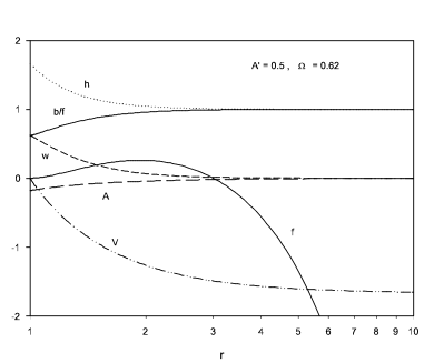
Figure 1: The profile of the metric and Maxwell functions for $r_{c}=3,r_{h}=1$ for $a_{h}^{\prime}=0.5$ and $\Omega=0.62$

The equations are cumbersome and it is not necessary to write them explicitely (see e.g. bd_2007 ), for the purpose of this report, we just write their overall structure which turns out to be :

$$\Lambda^{\prime}=0\ \ ,\ \ f^{\prime}=\dots\ ,\ \ ,b^{\prime\prime}=\dots\ \ ,\ \ h^{\prime\prime}=\dots\ \ ,\ \ w^{\prime\prime}=\dots\ \ ,\ \ V^{\prime\prime}=\dots\ \ ,\ \ a_{\varphi}^{\prime\prime}=\dots$$

where the dots symbolize functions of $f,b,h,w,a_{\phi}$ and of the derivative $b^{\prime},h^{\prime},w^{\prime},V^{\prime},a_{\phi}$. The fields $b,w,V$ can be arbitrarily rescaled according to

$$b\to\mu^{2}b\ \ ,\ \ w\to\mu w\ \ ,\ \ V\to\mu V+C\ \ ,\ \ \mu,C\ {\rm constants.}$$ (6)

After inspection of the equations and using this invariance, the boundary conditions for $r\in[r_{h},r_{c}]$ can be choosen according to

$$f(r_{h})=0\ \ ,\ b(r_{h})=0\ \ ,\ b^{\prime}(r_{h})=1\ \ ,\ \Gamma_{h}(r_{h})=0\ \$$ (7)

$$\ \ w(r_{h})=w_{h}\ ,\ \ V(r_{h})=0\ ,\ \ a^{\prime}_{\varphi}(r_{h})=a_{h}\ ,\Gamma_{A}(r_{h})=0$$ (8)

fixing the arbitrary scale of $b$. The parameters $w_{h}$, $a_{h}$ are fixed by hand and control the angular and magnetic moments respectively. At the cosmological horizon we set :

$$f(r_{c})=0\ \ ,\ \ b(r_{c})=0\ \ ,\ \ \Gamma_{h}(r_{c})=0\ \ ,\ \ \Gamma_{A}(r_{c})=0$$ (9)

completing the set of fourteen conditions. The conditions $\Gamma=0$ appearing in several boundary conditions are necessary conditions for the solutions to be regular at the horizon. For instance, we find

$$\Gamma_{A}(r)\equiv 4a_{\varphi}b^{\prime}h+r^{4}f^{\prime}(hw^{\prime}V^{\prime}+a_{\varphi}^{\prime}hww^{\prime}-a_{\varphi}^{\prime}b^{\prime})(r)$$ (10)

and an even more involved expression for $\Gamma_{h}$.

It should be stressed that the functions $w,b,V$ have to be renormalized after the integration on $[r_{h},\infty]$ in such a way that space-time is asymptotically de Sitter. In particular

$$b(r)=-\Lambda r^{2}+1+O(1/r^{2})\ \ \ \ {\rm for}\ \ r\to\infty$$

As a consequence, it turns out to be impossible (at least it is extremely lengthy) to study the solutions for fixed charge $Q$ and varying $\Omega$. The best way to study the domain of existence of solutions in the $a_{h}$–$\Omega_{h}$ plane consists in fixing the constant $a_{h}$ and vary the parameter $w_{h}$. After the suitable renormalisation of $b(r),w(r),V(r)$, families of rotating solutions with $a_{h}$ fixed can finally be constructed. A typical solution is shown in Fig.1. The numerical calculations further indicate the following features :
(i) For fixed $a_{h}$ and varying $w_{h}$, black holes exist only on a finite interval of the horizon angular velocity $\Omega$.
(ii) In the critical limits, solutions converge to extremal black holes, i.e. with $f(r_{h})=0$, $f^{\prime}(r_{h})=0$. These statements are illustrated by Fig. 2 .

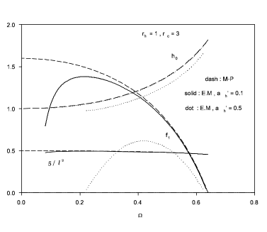
Figure 2: Some metric parameters and the parameter $\ell^{2}$ as functions of $\Omega$ for $r_{c}=3,r_{h}=1$ and for several values of $a_{h}^{\prime}$

Let us remark that the value $1/\ell^{2}$ turns out to depend only weakly on $\Omega$; it can therefore be considered that the family of rotating solutions constructed with fixed $r_{h},r_{c}$, $a_{h}$ correspond to $\Lambda$ nearly constant. The numerical results further indicate that, while approaching the boundary of the domain of existence of the black holes, the event horizon $r_{h}$ becomes extremal. This makes the numerical analysis difficult. However, extremal solutions can be constructed directly by implementing the following trick: (i) we introduce an arbitrary scale, say $\alpha$ for the Maxwell field $a_{\varphi}$ and supplement the system with an equation $d\alpha/dr=0$, (ii) we take advantage of the extra equation to replace the boundary conditions $f(r_{h})=0$, $a^{\prime}_{\phi}(r_{h})=a_{h}$ by $f(r_{h})=0,df/dr(r_{h})=0$, $db/dr(r_{h})=0$. This produces extremal solutions with a definite value of $\alpha$.
Physical quantities: Asymptotic global charges can be associated to each Killing vector of the metric. Using standard results Balasubramanian:1999re ; Brown:1993 ; ghezelbash_mann , the mass-energy $E$ and the angular momentum $J$ of the solutions can be computed. These physical quantities depend crucially on the asymptotics of the solutions. After some computation we obtain

$$b(r)=-\epsilon\frac{r^{2}}{\ell^{2}}+1+\frac{\alpha}{r^{d-3}}+O(1/r^{2d-6})\ \ ,\ \ f(r)=-\epsilon\frac{r^{2}}{\ell^{2}}+1+\frac{\beta}{r^{d-3}}+O(1/r^{d-1}),$$ (11)

$$h(r)=r^{2}(1+\epsilon\frac{\ell^{2}(\beta-\alpha)}{r^{d-1}}+O(1/r^{2d-4}))\ \ ,\ \ w(r)=\frac{\hat{J}}{r^{d-1}}+O(1/r^{2d-4}).$$ (12)

where $\epsilon=\pm$ denotes the sign of the cosmological constant. From these expansions, the mass and angular momentum can be computed :

$$E=\frac{V_{d-2}}{16\pi G_{d}}(\beta-(d-1)\alpha),~{}~{}J=\frac{V_{d-2}}{8\pi G_{d}}\hat{J}\ .$$ (13)

The dependence of $E,J$ on the angular velocity at the horizon $\Omega$ is illustrated in Fig. 3.

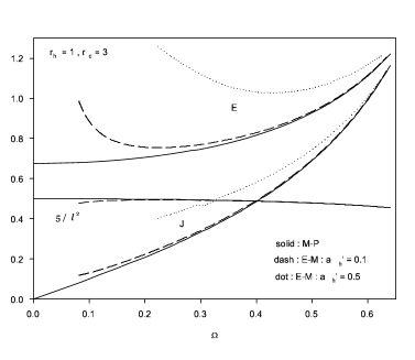
Figure 3: Mass and Angular momentum of the $\Lambda>0$ Black holes for $r_{c}=3$, $r_{h}=1$ as function of the angular velocity $\Omega$

Conserved quantities can be defined at the cosmological horizons as well. Smarr formulae relating them have been obtained bd_2008 .

II.4 Charged, rotating black holes with $\Lambda\leq 0$

Solutions with $\Lambda=0$ are constructed numerically in Kunz:2006eh and in knlr where the isotropic coordinate is used toparameterizee the metric. Charged, rotating black holes with $\Lambda<0$ are constructed in knlr also using the isotropic coordinate. We reconsidered several of these solutions using Schwarzschild coordinates. It is worth stressing, however, that the patterns of solutions look different when solving the equations in the isotropic coordinate, say $y$ with $y_{h}$ fixed and in Schwarzschild coordinates $r$, with $r_{h}$ fixed, respectively. The pattern obtained for the case $\Lambda<0$ (i.e. with $r_{h}$ fixed and $\Lambda$ fixed) is very similar to the one suggested by Fig 3. In particular, the solutions terminate into an extremal black hole (the event horizon is extremal) when a maximal value of $\Omega$ is reached. The profiles of such an extremal black hole are presented in Fig. 4.

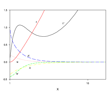
Figure 4: Extremal rotating black hole with $\Omega=0.2$ and $\Lambda<0$

III Black strings with cosmological constant

III.1 General setting

In this section, we discuss black string solutions of the vacuum Einstein equations in $d$-dimensions and in the presence of a cosmological constant. For this type of black objects, one of the spacelike dimensions of the space-time manifold, say $z\equiv x_{d-1}$, plays a special role : space-time is chosen, a priori, as a warped product of a $d-1$-dimensional black hole metric with the extra-dimension $z$ which is assumed to be periodic with a period $L$. The horizon of the black string then has a topology of $S_{d-3}\times S_{1}$. The simplest case consists in assuming the metric to be independent of $z$, the corresponding solutions are then called uniform black strings (UBS). The metric has the form

$$ds_{bs}^{2}=a(r)dz^{2}+ds^{2}$$ (14)

where $ds^{2}$ is given by (II.1) (see previous section).
In the case $\Lambda=0$ non-uniform black strings are known to be unstable gl for sufficiently large values of $L$. Stable solutions can further beconstructedd with a metric depending on $r$ and $z$. They are called non-uniform black strings wiseman .
In the absence of the electromagnetic field and of rotation, substituting the metric (14) in the Einstein equations leads to a system of three differential equations with the structure:

$$f^{\prime}=Q_{1}(f,a,b,b^{\prime},\Lambda)\ \ ,\ \ ,\ \ a^{\prime}=Q_{2}(f,a,b,b^{\prime},\Lambda)\ \ ,\ \ b^{\prime\prime}=Q_{3}(f,a,b,b^{\prime},\Lambda)\ \ \ \$$ (15)

the full expressions of the $Q_{1,2,3}$ are given in mrs and

$$w(r)=0\ \ ,\ \ h(r)=r^{2}\ \ ,\ \ g(r)=r^{2}$$ (16)

We first discuss the solutions for $\Lambda<0$.

III.2 Uniform solutions: $\Lambda<0$

We consider non-extremal black string solutions possessing a regular event horizon at $r=r_{h}$. Near this horizon, the fields can be expanded according to

$$a(r)=a_{h}+O(r-r_{h}),~{}b(r)=b_{1}(r-r_{h})+O(r-r_{h})^{2},~{}f(r)=f_{1}(r-r_{h})+O(r-r_{h})^{2},{~{}~{}~{}~{}}$$ (17)

with all coefficients fixed by the parameters $a_{h}$, $b_{1}$. Since the coordinates $t$ and $z$ can be rescaled arbitrarily, the equations are invariant under arenormalizationn the functions $a(r)$ and $b(r)$. Using this arbitrariness one can specify the four boundary conditions for a black string according to :

$$f(r_{h})=0\ \ ,\ \ a(r_{h})=1\ \ ,\ \ b(r_{h})=0\ \ ,\ \ b^{\prime}(r_{h})=1$$ (18)

so that the equations can be treated as a Cauchy problem. The profiles for $a(r)$ and $b(r)$ obtained in this way need, however, to be rescaled in such a way that the metric is asymptotically de Sitter, Minkowski or Anti–de–Sitter (according to the value of the cosmological constant). The asymptotic expansion of the solutions leads to

$$f(r)=\frac{(d-1)(d-4)}{(d-2)(d-3)}+\frac{r^{2}}{\ell^{2}}+\dots\ \ ,\ \ a(r)=(\frac{d-4}{d-3})+\frac{r^{2}}{\ell^{2}}+\dots\ \,\ \ b(r)=(\frac{d-4}{d-3})+\frac{r^{2}}{\ell^{2}}+\dots$$ (19)

where the dots denote the various $1/r$ corrections given e.g. in br_2008 .

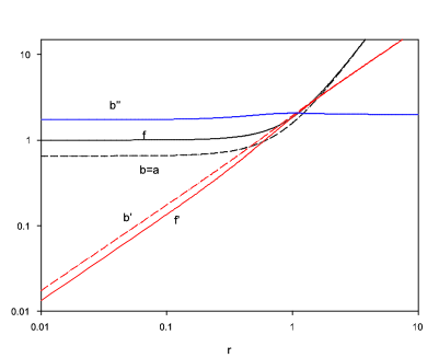
Figure 5: Profiles of the regular solution for $d=8$

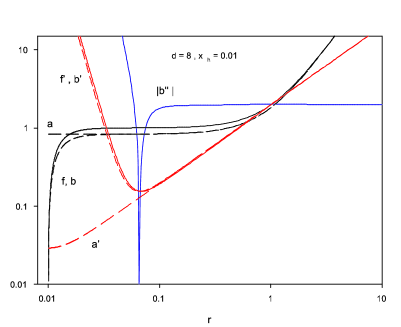
Figure 6: Profiles of an AdS black string for $r_{h}=0.01$

For $\Lambda<0$, the equations admit, to our knowledge, no explicit solutions. Black strings were constructed numerically in mrs . The numerical results strongly suggest that they exist for arbitrary values of $r_{h}$. In the limit $r_{h}\to 0$, a soliton-type solution is approached. The limiting solution has $a(r)=b(r)$ and is regular at the origin ($f(0)=1$, $f^{\prime}(0)=b^{\prime}(0)=0$) and approaches Anti–de–Sitter (AdS) space-time for $r\to\infty$. The convergence of the black string to the soliton is pointlike outside the origin; that is to say that, in the limit $r_{h}\to 0$, the quantities $f^{\prime}(r_{h}),b^{\prime}(r_{h})$ become infinite while $a(r_{h})$ and $a^{\prime}(r_{h})$ converge to $1$ and $0$ respectively. Profiles of the regular solution and of an AdS black string corresponding to $r_{h}=0.01$ are shown in Fig.5 and Fig.6, respectively. (Note that the spike presented by $|b^{\prime}|$ in this figure is an effect of the logarithmic scale.)

Rotating black string. The rotating solutions have $w(r)>0$ and $g(r)\neq r^{2}$. The results of brs_2007 show that they exist for arbitrarily large values of $w(r_{h})$. A typical profile of a uniform rotating AdS black string solution is presented in Fig.7

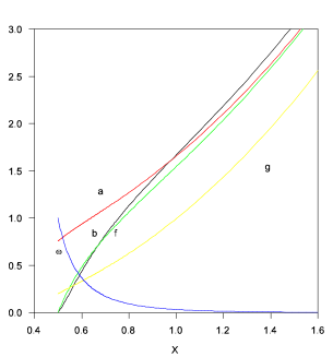
Figure 7: Profile of the metric functions for a rotating AdS black string for $r_{h}=1$, $\Omega=1$

Physical quantities. AdS black strings can be characterized by conserved asymptotic charges : their mass $M$ and tension $\cal T$. Using the formalism explained in detail in mrs they can be extracted from the asymptotic decay of the metric functions:

$$M=\frac{\ell^{d-4}}{16\pi}LV_{d-3}[c_{z}-(d-2)c_{t}]+M_{c}(d)$$ (20)

$$a(r)=\dots+c_{z}(\frac{\ell}{r})^{d-3}+\dots\ ,\ b(r)=\dots+c_{t}(\frac{\ell}{r})^{d-3}+\dots$$ (21)

Moreover, thermodynamical quantities characterizing the solutions can also be determined. They depend on the value of the metric at the event horizon $r_{h}$ : the entropy $S$

$$S=\frac{1}{4}r_{h}^{d-3}LV_{d-3}\sqrt{a(r_{h})}$$ (22)

and Hawking temperature $T_{H}$

$$T_{H}=\frac{1}{4}\sqrt{\frac{b^{\prime}(r_{h})}{r_{h}}((d-4)+(d-1)r_{h}^{2}/\ell^{2})}$$ (23)

“Local thermodynamical stability” is related to the sign of the heat capacity

$$C=T_{H}\frac{\partial S}{\partial T_{H}}\ \ ,\ \ {\rm for\ \ }L{\rm\ \ fixed}$$ (24)

Solutions with $C>0$ are thermodynamically stable while those with $C<0$ are unstable. It is worth stating that asymptotically flat black strings with different $r_{h}$ are related by a rescaling of the radial coordinate. On the contrary, AdS black strings with $\Lambda$ fixed and $r_{h}$ varying form a family of intrinsically different solutions. From the analysis of mrs , it turns out that the solutions obtained by varying $r_{h}$ form two branches distinguished thermodynamically: solutions with small $r_{h}$ have $C>0$, solutions with large $r_{h}$ have $C<0$. This is illustrated in Fig. 8 for $d=5$ and $\Lambda=-1$.

Figure 8: Entropy as function of $T_{H}$ for the family of black strings corresponding to $\Lambda=-1$ and $d=5$

Charged black strings. To finish this section, let us point out that charged black strings with $A=V(r)dt$ were considered in brs_2007 as well. The Maxwell equation can be solved directly, leading to:

$$F^{tr}=\frac{q}{r^{d-3}}\sqrt{\frac{f(r)}{a(r)b(r)}}\ \ ,\ \ q={\rm constant}$$

Charged black strings exist for $r_{h}>r_{h,min}>0$ for $q>0$.

As main result of our analysis of the thermodynamical properties of the solutions, let us point out that charge and rotation change the thermodynamical stability pattern of the black strings. For the families of solutions obtained by varying $r_{h}$ but fixed $L$ , $Q$ (in the case of charged black strings ) and for fixed $L$ , $J$ (in the case of spinning black strings, corresponding to a Grand canonical ensemble) the unstable branch has a tendency todiminishh and disappear for large enough values of the charge or of the angular momentum.

Figure 9: Entropy as function of $T_{H}$ for families of black strings corresponding to $\Lambda=-1$ and $d=5$ with fixed electric charge

Figure 10: Entropy as function of $T_{H}$ for families of black strings corresponding to $\Lambda=-1$ and $d=5$ with fixed angular momentum

III.3 Uniform solutions : $\Lambda>0$

Solving the equations for a positive cosmological constant bd_2007_bis , we find no solutions possessing both a regular horizon at $r=r_{h}$ and being asymptotically de Sitter, i.e.

$$f(r),a(r),b(r)\to-\Lambda r^{2}+{\rm constant}+O(1/r^{2})\ \ ,\ \ {\rm for}\ \ \ r\to\infty$$ (25)

As pointed out above, imposing a regular horizon at $r=r_{h}$ needs only conditions at the horizon. Extrapolating the initial data up to $r\to\infty$ reveals that the solution evolves asymptotically into a configuration such that

$$a(r)\to r^{\alpha}\ ,\ b(r)\to r^{\alpha}\ ,\ f(r)\to r^{\gamma}$$ (26)

where the parameters $\alpha$, $\gamma$ depend on $d$ :

$$\alpha=-2(d-3)-\sqrt{2(d-2)(d-3)},\gamma=2(d-2)+\sqrt{2(d-2)(d-3)}\ \ .$$ (27)

The form (26) corresponds to one possible asymptotic behaviour of the solutions, the other possibility is de Sitter. A solution for $r_{h}=0.5$ (including rotation) is presented in Fig. 11. Examining the Kretschmann scalar reveals that the solution with the asymptotics (26) are singular at $r=\infty$. Along with the case $\Lambda<0$, solutions regular at the origin exist as well, but have the asymptotics (26). To finish this discussion, we mention that imposing a regular cosmological horizon at $r=r_{c}$ leads to the absence of a regular horizon at finite distance and to a naked singularity at the origin.

Black strings with $\Lambda\neq 0$ therefore lead to a situation where no analytical continuation of the $\Lambda<0$ solutions into the $\Lambda>0$ domain can be established; it is tempting to relate this result to the absence of explicit solutions.

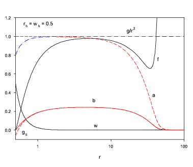
Figure 11: Solution with $r_{h}=0.5$, $\Omega=0.5$, $d=5$ and $\Lambda>0$

III.4 Stability of AdS black strings

As mentioned above, the extra dimension of space-timeparameterizedd by $z$ is assumed to be periodic with period $L$, i.e. $z\in[0,L]$. One of the most striking facts about asymptotically flat black strings is that they present an instability gl for large values of $L$, as discovered by Gregory and Laflamme (GL). It is therefore natural to determine whether AdS black strings also have an instability of the GL type and to attempt to relate this eventual instability to the thermodynamical instability discussed in previous sections. In this framework, it is interesting to check whether the following conjecture formulated by Gubser and Mitra gm is fulfilled for the ADS black strings : ”For a black brane solution to be free of dynamical instabilities it is necessary and sufficient for it to be locally thermodynamically stable.”
Digression to the electroweak model. To some extend theoccurrencee of instabilities of uniform black strings and the emergence of non–uniform (i.e. $z$-depending) solutions can be compared with an older problem: the sphaleron instability. The classical equations of the SU(2)$\times$ U(1) Yang-Mills-Higgs (the bosonic sector of the electroweak Lagrangian) admit a solution: the Klinkhamer-Manton (KM) sphaleron km_1984 . The study of the instability of the sphaleron can be performed by linearizing the equations about the sphaleron with respect to a time-dependent fluctuation, i.e.

$$\Phi(t,r)=\Phi_{KM}(r)+e^{\omega t}\eta(r)\longrightarrow H\eta=\omega\eta$$ (28)

where $\Phi_{KM}$ symbolizes the sphaleron configuration. All physical parameters can be scaled away from the equations apart from the Higgs-particle mass $M_{H}$ which is left as a free parameter (we assume the limit of vanishing Weinberg angle $\theta_{w}=0$). It was shown bk_1988 ; yaffe_1988 ; bk_1990 that the linearized equations lead to a spectral problem with spectral parameter $\omega$ and that normalizable fluctuations exist for specific eigenvalues $\omega(M_{H})$. For a series of critical values $M_{H,c}$, we have zero modes $\omega(M_{H,c})=0$ and the number of negative eigenvalues depends on $M_{H}$. As a consequence new solutions exist for $M_{H}\geq M_{H,c}$ bifurcating from the KM sphaleron. Because these new solutions appear in pairs, related to each other by parity, we called them bisphaleron. The analogies between the 20–year old bisphaleron and the more recent non–uniform black strings can be seen as follows :

• Yang-Mills-Higgs equations $\longrightarrow$ Einstein equations for $d>4$.

• Higgs field mass $M_{H}$ $\longrightarrow$ Length of the co-dimension $L$.

• KM-sphaleron $\longrightarrow$ Uniform Black String (Schwarzschild).

• bisphaleron $\longrightarrow$ non–uniform black string.

• Breaking of parity $\longrightarrow$ Breaking of the translation symmetry in $z$.

• Morse theorem + Catastrophe theory $\longrightarrow$ Gubser-Mitra conjecture.

Coming back to the GL-instability for AdS black strings, we consider a deformation of the metric which we parametrize like in Gubser:2001ac :

$$ds^{2}=-b(r)e^{2A(r,z)}dt^{2}+e^{2B(r,z)}\left(\frac{dr^{2}}{f(r)}+a(r)dz^{2}\right)+r^{2}e^{2F(r,z)}d\Omega_{d-3}^{2}\ \ ,$$ (29)

assuming no time-dependence of the metric fields. That is to say that we specialize in the zero-mode, i.e. $\Omega=0$ where $\Omega$ is used in gl . The functions $A,B,C$ encode the deviations with respect to the uniform metric and depend on $z$ and $r$. Using the periodic conditions assumed in $z$, the fluctuations can be expanded in Fourier series :

$$X(r,z)=\epsilon X_{1}(r)\cos(kz)+\epsilon^{2}(X_{0}(r)+X_{2}(r)\cos(2kz))+O(\epsilon^{2})\ ,\ k\equiv\frac{2\pi}{L}$$

where $X$ stands for $A,B,F$ and $\epsilon$ denotes an infinitesimal parameter. Extracting the terms linear in $\epsilon$ from the Einstein equations leads to a system of linear differential equations in $A_{1}(r),B_{1}(r),F_{1}(r)$. Instead of writing these lengthly equations (they can be found in bdr_2007 ), we point out a few of their properties :

• The “potentials”: the functions $a(r),b(r),f(r)$ are known only numerically.

• The perturbations $X_{1}(r)$ should vanish asymptotically.

• The function $B_{1}(r)$ can be eliminated from the system.

• Regularity at $r=r_{h}$ leads to two conditions of the form $\Gamma(A,C,A^{\prime},C^{\prime})(r=r_{h})=0$.

• Special values of $k^{2}$ have to be determined such that boundary conditions are fulfilled up to a global factor : it is an eigenvalue problem.

• A rescaling of the radial coordinate can be used to set either $r_{h}$ or $\Lambda$ to a canonical value, e.g. $\Lambda=-1$.

• Solutions with $k^{2}>0$ are unstable, $k^{2}<0$ are stable.

Fig. 12 summarizes our results for the critical value of $k$ as a function of the event horizon value $r_{h}$ for several values of $d$. The comparison between the entropy of the solution and the eigenvalue $k^{2}$ as functions of the Hawking temperature $T_{H}$ is reported in Figs.13 and 14 for $d=5,8$ respectively. These figures clearly show that the solutions having $k^{2}>0$ have a negative heat capacity and are therefore unstable, while solutions with $k^{2}<0$ have a positive heat capacity and are stable. The fact that the change of sign of $k^{2}$ coincides with the change of sign of the heat capacity indicates that the GM conjecture is fulfilled for AdS black strings.

Figure 12: The value of $k^{2}$ as a function of $r_{h}$ for $d=5,6,8$ and $\Lambda=-1$

Figure 13: The entropy $S$ and the eigenvalue $k^{2}$ as function of $T_{H}$ for $d=5$. The figure shows that the GM conjecture is obeyed.

Figure 14: The entropy $S$ and the eigenvalue $k^{2}$ as function of $T_{H}$ for $d=8$. The figure shows that the GM conjecture is obeyed.

III.5 Non-uniform (EGB) AdS black strings.

The results of the previous section strongly suggest that non-uniform black strings with AdS asymptotics should exist as well. To construct such solutions, the above spherically symmetric ansatz has to be generalized in order to allow the metric to depend on the radial variable $r$ and on the extra dimension denoted here by $y$.

For the calculations, it is convenient to use an alternative parametrisation of the radial variable and to work with a new one, $\tilde{r}$, defined through

$$ds^{2}=-e^{2A}\tilde{b}dt^{2}+\tilde{g}(\tilde{r})e^{2C}d\Omega^{2}+e^{2B}(\frac{1}{\tilde{f}}\frac{\tilde{r}^{2}}{\tilde{g}}dr^{2}+\tilde{a}dy^{2})$$ (30)

where the ”tilde” refers to quantities depending on the radius $\tilde{r}$. The dependence on $y$ appears through the functions $A,B,C$. Practically, we use $\tilde{g}=\tilde{r}^{2}+r_{h}^{2}$. The event horizon thencorrespondss to $\tilde{r}=0$ and the relations $\tilde{f}(\tilde{r})=f(r)$,$\tilde{a}(\tilde{r})=a(r)$,$\tilde{b}(\tilde{r})=b(r)$ hold.

The system of partial differential equations for $A,B,C$ has to be solved with the following boundary conditions

$$\partial_{r}A(0,y)=\partial_{r}C(0,y)=0\ \ ,\ \ B(0,y)-A(0,y)=\alpha\ \ ,\ \ \ X(\infty,y)=0$$ (31)

$$\partial_{y}X(r,0)=0\ \ ,\ \ \partial_{y}X(r,L)=0\ \ ,\ \ X=A,B,C$$ (32)

where the parameter $\alpha$ will enforce the deformation with respect to uniform configurations. The solutions that we are looking for are periodic for $y\in[0,L]$ and present a mirror symmetry $y\to L-y$. The corresponding equation was solved numerically in the case $\Lambda=-1$, $r_{h}=1$ corresponding to $k_{cr}\approx 1.143$ (determining the critical radius $L_{cr}=2\pi/k_{cr}$) and for several values of $\alpha$. For the numerical integration, we used a compactified variable $x=\tilde{r}/(1+\tilde{r})$ and $z=y/L_{cr}$. The square $(x,z)\in[0,1]\times[0,1]$ was discretized with grids of 80 $\times$ 80 points.

Profiles of the deformation functions $A,B,C$ are given in several figures. In Fig.15 the deviation of the $g_{tt}$ metric component at the horizon is given as function of $y$ for several values of $\alpha$. Similar plots of the quantity $\exp(B+C)$ are given in Fig.16. This quantity is directly relevant for the calculation of the entropy of the non-uniform black strings. Finally, the quantity $\exp(C)$, encoding the deformation parameter introduced e.g. in Gubser:2001ac is given in Fig. 17. The figures reveal that, for $\alpha$ increasing, the deformation becomes very pronounced at $y=L/2$. The grids used where not sufficient to get reliable solutions for $\alpha>0.9$. More detailed studies of these non-uniform solutions are presented in delsate_2008 .

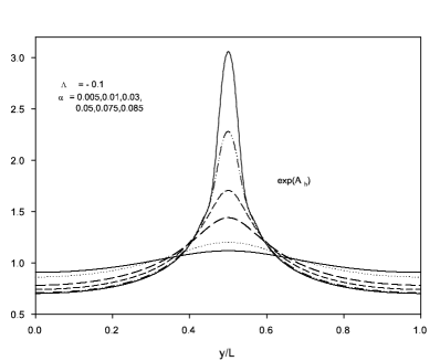
Figure 15: The profiles of the quantity $\exp A$ evaluated at the horizon for $\Lambda=-0.1$ and several values of $\alpha$ and $d=6$

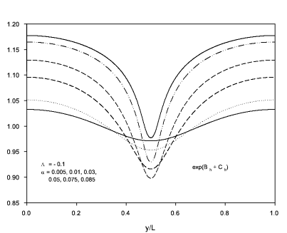
Figure 16: The profiles of the quantity $\exp B+C$ evaluated at the horizon for $\Lambda=-0.1$ and several values of $\alpha$ and $d=6$

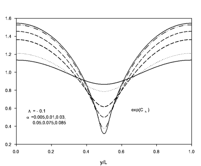
Figure 17: The profiles of the quantity $\exp C$ evaluated at the horizon for $\Lambda=-0.1$ and several values of $\alpha$ and $d=6$

The dependence of the solutions on the radial variable is further illustrated in Figs.18 and 19 correspondingg to $\alpha=0.8$) The functions $A$ and $C$ decrease monotonically to zero for $r\to\infty$. The behaviour of the combination $B+C$ is more involved since it presents a local maximum at an intermediate value $r=r_{m}$ for $y=L/2$ .

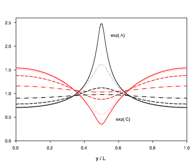
Figure 18: The profiles of the values $\exp A(x,y)$ (black lines) and $\exp C(x,y)$ (red lines) as functions of $y$ and for $x=0,0.2,0.4,0.6$ and $\Lambda=-0.1$

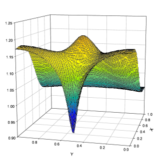
Figure 19: Two-dimensional plot of the function $\exp(B+C)(x,y)$ for $\alpha=0.8$ and $\Lambda=-0.1$

IV AdS black strings in Einstein-Gauss-Bonnet

So far, we presented blackobjectssoccurringg in minimal models for gravity, i.e. constructed within the minimal Einstein-Hilbert action. In higher dimensions, however, there exist more general choices of physically acceptable Lagrangians describing gravity. Low energy effective models descending from string theory contain such terms. It is therefore natural to pay attention to the influence of additional terms in the gravity sector on the classical solutions i.e. on black holes and black strings. The Gauss-Bonnet (GB) interaction is the first curvature correction to General Relativity from the low energy effective action of string theory. It is quartic in the metric and of second order in the derivatives.

IV.1 The Einstein-Gauss-Bonnet equations

In this section, we consider the Einstein-Gauss-Bonnet (EGB) action supplemented with a cosmological constant $\Lambda=-(d-2)(d-1)/2\ell^{2}$ :

$$I=\frac{1}{16\pi G}\int_{\mathcal{M}}~{}d^{d}x\sqrt{-g}\left(R-2\Lambda+\frac{\alpha}{4}L_{GB}\right),$$

$R$ is the Ricci scalar and

$$L_{GB}=R^{2}-4R_{\mu\nu}R^{\mu\nu}+R_{\mu\nu\sigma\tau}R^{\mu\nu\sigma\tau},$$

denotes the Gauss-Bonnet term. Variation of this action with respect to the metric results in the EGB equations:

$$R_{\mu\nu}-\frac{1}{2}Rg_{\mu\nu}+\Lambda g_{\mu\nu}+\frac{\alpha}{4}H_{\mu\nu}=0~{},$$

where

$$H_{\mu\nu}=2(R_{\mu\sigma\kappa\tau}R_{\nu}^{\phantom{\nu}\sigma\kappa\tau}-2R_{\mu\rho\nu\sigma}R^{\rho\sigma}-2R_{\mu\sigma}R_{\phantom{\sigma}\nu}^{\sigma}+RR_{\mu\nu})-\frac{1}{2}L_{GB}g_{\mu\nu}~{}.$$

It is useful to define an effective Anti-de-Sitter radius by means of

$$\ell_{c}=\ell\sqrt{\frac{1+U}{2}},~{}~{}{\rm~{}~{}with~{}~{}~{}~{}}U=\sqrt{1-\frac{\alpha(d-3)(d-4)}{\ell^{2}}},$$

This combination of $\ell$ and $\alpha$ indeed appears naturally in the asymptotic expansion of the solution and in the counterterm formalism discussed in the next section. The occurrence of $\ell_{c}$ in the equation has consequences on the solutions since it leads to the existence of an upper bound for the Gauss-Bonnet coefficient, $\alpha\leq\alpha_{max}=\ell^{2}/(d-3)(d-4)$ in the case of asymptotically AdS solutions.

IV.2 Counterterm Formalism

Several times in the previous sections of this manuscript we used tacitely the existence of regularizing counterterms which allow the theory to be well defined and finite. This is not misleading since these countertems do not affect the classical equations. Here, we will present their explicit form and illustrate their interest for the theory under investigation, i.e. the Einstein-Gauss-Bonnet model.

Let us first remark that the various solutions of the models considered here do not have a finite action because of the non-compact character of space-times with $\Lambda=0$ or $\Lambda<0$. In order to enforce finite numbers for the action, one technique consists in adding suitable counterterms to the original action Balasubramanian:1999re ; Brown:1993 . The counterterms are constructed in such a way that the full Lagrangians fulfill several requirements, namely:

• They depend on curvature invariants associated with the geometry at the boundary of space-time.

• They do not affect the equations.

• They are also infinite, in order to cancel the divergences of the basic action.

As a byproduct, the counterterms lead to a boundary stress tensor $T_{a}^{b}$ which allows in particular to define conserved quantities like mass and angular momentum ghezelbash_mann .
The counterterms are known in the case of the Einstein-Hilbert action; we present here the generalization of this result to the case of the Einstein-Gauss-Bonnet action.

For $d<8$ and even, the appropriate counterterms are given by br_2008

$$I_{\mathrm{ct}}^{0} = \frac{1}{8\pi G}\int_{\partial\mathcal{M}}d^{d-1}x\sqrt{-\gamma}$$

$$\bigg{\{} - (\frac{d-2}{\ell_{c}})(\frac{2+U}{3})-\frac{\ell_{c}\mathsf{\Theta}\left(d-4\right)}{2(d-3)}(2-U){\mathsf{R}}$$

$$-\frac{\ell_{c}^{3}\mathsf{\Theta}\left(d-6\right)}{2(d-3)^{2}(d-5)}$$

$$\left[U\bigg{(}{\mathsf{R}_{ab}\mathsf{R}^{ab}}-\frac{d-1}{4(d-2)}{\mathsf{R}^{2}}\bigg{)}-\frac{d-3}{2(d-4)}(U-1){L_{GB}}\right]\bigg{\}},$$

where the quantity $U$ is defined above and

• $\gamma$ in the induced metric of the boundary of space-time.

• $\mathsf{R}$, $\mathsf{R}^{ab}$ and $L_{GB}$ are the curvature, the Ricci tensor and the Gauss-Bonnet term associated with $\gamma$.

• $\mathsf{\Theta}(x)$ is the step-function with $\mathsf{\Theta}\left(x\right)=1$ provided $x\geq 0$, and zero otherwise.

Up to the cases we have addressed, it turs out that these counterterms appears as a truncated series of powers of $R_{abcd}$ and $\ell_{c}$. We guess this can be generalized to arbitrary values of $d$ although we have no formal proof of this. Let us finally stress that the corresponding counterterms of Einstein gravity are recovered for $\alpha\to 0$ (i.e. $U\to 1$) and that for odd values of $d$ the expression is more involved.

IV.3 Black string and thermodynamical properties

We now discuss the black string solutions of the Einstein-Gauss-Bonnet (EGB) equations. At first sight, these solutions appear as smooth deformations of the Einstein black strings, although the deviation from the pure Einstein black strings is systematically significant even for infinitesimal values of $\alpha$. This is seen in Fig. 20.

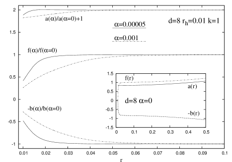
Figure 20: Comparison of profiles of E-BS and EGB-BS for small values of $\alpha$ and $d=8$

One striking property is that the Smarr relation available for $\alpha=0$ is obeyed for $\alpha>0$

$$M+{\cal T}L=T_{H}S$$ (33)

The effect of the Gauss-Bonnet (GB) terms appears more drastically when looking at the curve $S(T_{H})$, (shown in Fig. 21) demonstrating the influence of the GB interaction on the thermodynamical properties: the unstable branch of solutions occurring for $\alpha=0$ disappears progressively in favour of a branch of thermodynamically stable solutions when the Gauss-Bonnet coupling constant $\alpha$ increases.

Figure 21: The entropy $S$ as a function of $T_{H}$ for different values of $\alpha$ and $d=6$

IV.4 Domain of existence

In this section, we discuss the domain of existence of the EGB black strings in terms of the parameters $\alpha,r_{h}$ and $\Lambda$. In the case $\Lambda=0$, the black strings solutions are discussed in kobayashi_tanaka:2005 for $d=5$. Besides black strings, $M_{d-1}\times S_{1}$ constitutes a regular solution of the equations on $r\in[0,\infty]$ irrespectively of the value of $\alpha$ ($M_{p}$ denotes $p$-dimensional Minkowski space).

As mentioned above, for $\Lambda\neq 0$, the black strings of the vacuum Einstein equations exist for arbitrary values of $r_{h}$ and approach soliton-type solution in the limit $r_{h}\to 0$. The limiting solution has $a(r)=b(r)$, it is regular at the origin ($f(0)=1$, $f^{\prime}(0)=b^{\prime}(0)=0$) and approaches Anti–de–Sitter space-time for $r\to\infty$. The convergence of the black string to the soliton is therefore pointlike outside the origin; that is to say that, for $r_{h}\to 0$, the quantities $f^{\prime}(r_{h}),b^{\prime}(r_{h})$ become infinite while $a(r_{h})$ and $a^{\prime}(r_{h})$ converge to $1$ and $0$ respectively. The corresponding curves are shown (for $d=6$) (red lines) in Fig. 22.
Determining the domain of existence of black strings in the EGB case needs a detailed analysis of the behaviour of solutions in the limit $r_{h}\to 0$. EGB black strings were studied in br_2008 but details about their behaviour in the $r_{h}\to 0$ limit will be reported here. As we will see, the pattern crucially depends on the number of dimensions.

IV.4.1 Case d=5

In this case, the solutions exist only on a sub-domain of the $r_{h}$-$\alpha$ plane limited by $\alpha<\alpha_{m}$ with $\alpha_{m}=r_{h}^{2}/(2(1+r_{h}^{2}))$. Performing the expansion (17) about the event horizon, leads for the parameter $f_{1}$ to

$$f_{1}=\frac{r_{h}^{2}(\ell^{2}+2\alpha)}{\ell^{2}\alpha}-\frac{1}{\ell^{2}\alpha}\sqrt{(\ell^{2}-2\alpha)\left(r_{h}^{2}(\ell^{2}-2\alpha)-2\ell^{2}\alpha\right)},$$ (34)

which clearly implies that real solutions exist for $r_{h}>\ell/\sqrt{\ell^{2}/(2\alpha)-1}$.

IV.4.2 Case d=6

The expression (34) of $f_{1}$ for generic $d$ is much more complicated and does not bring definite information about the domain for $d>5$. The domain of existence of 6-dimensional EGB black string is more tricky, as illustrated by Figs. 22 and 23. First, let us mention that the solutions exist only for $\alpha<1/6$ which constitute the main critical value. To understand the pattern of the solutions, it is worth looking at the parameters $f^{\prime}_{h},a^{\prime}_{h},b^{\prime}_{h}$. For a fixed positive value of $\alpha$ the quantities $a^{\prime}_{h},b^{\prime}_{h},f^{\prime}_{h}$ behave like in the $\alpha=0$ case (red lines) for large $r_{h}$. When $r_{h}$ diminishes, they deviate from their values in the Einstein case, they attain a maximum and then all decrease to zero for $r_{h}\to 0$. This suggests that the EGB black strings approach a configuration with a singularity at the origin in the limit $r_{h}\to 0$. Figure (23) further illustrates how the parameters $f^{\prime}(r_{h}),a(r_{h}),a^{\prime}(r_{h}),b^{\prime}(r_{h})$ vary as functions of $\alpha$ for two different values of the horizon. For large horizon values, e.g. $r_{h}\sim 0.5$, these variations are small. For smaller $r_{h}$ the variations are more significant and some oscillations are observed.

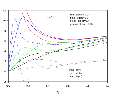
Figure 22: The parameters at the horizon of some d=6 solutions as functions of $r_{h}$ for two different values of $\alpha$

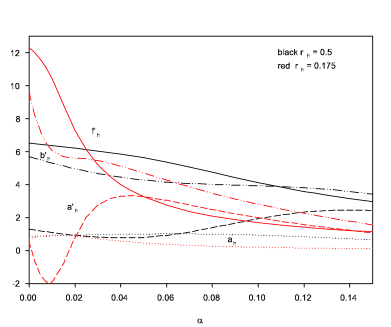
Figure 23: Some parameters at the horizon of some d=6 solutions as functions of $\alpha$ for two different values of $r_{h}$: $f^{\prime}$ (solid), $a$ (dots), $a^{\prime}$ (dash), $b^{\prime}$ (dot-dash)

These results reveal a non-perturbative character of the Gauss-Bonnet coupling constant : a small variation of $\alpha$ leads to a significant change in the profiles of the metric functions and especially of their derivatives. The correction is likely non polynomial and cannot be treated perturbatively.

IV.4.3 Case d=8

The analysis of the $r_{h}\to 0$ limit in the case $d=8$ is even more subtle and undefinite. Our numerical results do not confirm the existence of a definite solution in this limit (even presenting a singularity at the origin). It should be stressed that it turns out to be extremely difficult to construct numerical solutions for $\alpha>0$ and $r_{h}<0.01$. Examining the behaviour of the derivatives of $f,b$ at the horizon (say $f^{\prime}_{h}$ and $b^{\prime}_{h}$) for fixed positive $\alpha$ and varying $r_{h}$ reveals that these quantities increase when $r_{h}$ decreases, like for Einstein-black strings in $d=6$ (see Fig. 22). The situation is, however, different because the value $a(r_{h})$ (see Fig. 24) varies non monotonically. It develops some oscillations when both $\alpha$ and $r_{h}$ are small. Our results suggest that these oscillations become more and more pronounced when the value of $r_{h}$ decreases. This makes it not easy to construct these solutions numerically and it turns out impossible to have proper insight into the nature of the limiting configuration.

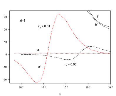
Figure 24: Values of $a_{h}$ and $a^{\prime}_{h}$ as functions of $\alpha$ for different values of $r_{h}$

V Conclusions

We have constructed black holes and black strings solutions within several models in the presence of a cosmological constant. Up to our knowledge, the extensions that we have discussed do not allow explicit solutions of the equations. We therefore used numerical methods to solve the equations. We hope these results contribute to a more general understanding of the classification of solutions of the Einstein equations in $d>4$.

Acknowledgments. It is a pleasure to acknowledge J. Kunz and C. Lämmerzahl for their invitation to the Heraeus Seminar in Bremen in August 2008. I am also grateful to T. Delsate and E. Radu for their collaboration on the topic.

References

- (1) V. A. Rubakov and M. E. Shaposhnikov, Phys. Lett. B 125 (1983) 136; 125 (1983) 139.
- (2) L. Randall and R. Sundrum, Phys. Rev. Lett. 83 (1999), 3370; id. 4690.
- (3) F. R. Tangherlini, Nuovo Cimento 77, 636 (1963).
- (4) R. C. Myers and M. J. Perry, Ann. Phys. (N. Y.) 172 (1986) 304.
- (5) R. Gregory and R. Laflamme, Phys. Rev. Lett. 70 (1993) 2837.
- (6) R. Emparan and H. Reall, Class.Quant.Grav.23 (2006) R169.
-
(7)
S. Perlmutter et al. [Supernova Cosmology Project Collaboration],
Nature 391 (1998) 51,
A. G. Riess et al. [Supernova Search Team Collaboration], Astron. J. 116 (1998) 1009. - (8) E. Witten, Adv. Theor. Math. Phys. 2 (1998) 253.
- (9) J. M. Maldacena, Adv. Theor. Math. Phys. 2 (1998) 231, [Int. J. Theor. Phys. 38 (1999) 1113].
-
(10)
G. W. Gibbons, H. Lu, D. N. Page and C. N. Pope,
Phys. Rev. Lett. 93 (2004) 171102.
G. W. Gibbons, H. Lu, D. N. Page and C. N. Pope, J. Geom. Phys. 53 (2005) 49. - (11) D. Klemm and W. A. Sabra, JHEP 0102 (2001) 031.
- (12) M. Cvetic, H. Lu and C. N. Pope, Phys. Lett. B598 (2004) 273-278.
- (13) Y. Brihaye and T. Delsate, Class. Quant. Grav. 24 (2007) 4839.
- (14) V. Balasubramanian and P. Kraus, Commun. Math. Phys. 208 (1999) 413.
- (15) J. D. Brown and J. W. York, Phys. Rev. D47 (1993) 1407.
- (16) D. Klemm, Nucl.Phys.B 625 (2002) 295.
- (17) A. M. Ghezelbash and R. B. Mann, JHEP 0201 (2002) 005.
- (18) Y. Brihaye and T. Delsate, ”Charged-Rotating Black Holes in Higher-dimensional (A)DS-Gravity”, ArXiv:0806.1581.
- (19) J. Kunz, F. Navarro-Lerida and J. Viebahn, Phys. Lett. B 639 (2006) 362.
- (20) A. N. Aliev, Phys.Rev. D74 (2006) 024011.
- (21) J. Kunz, F. Navarro-Lerida and E. Radu, Phys.Lett.B649: (2007) 463.
- (22) A. N. Aliev, Phys.Rev.D75 (2007) 084041.
- (23) S. S. Gubser, Class. Quant. Grav. 19 (2002) 4825
- (24) T. Wiseman, Class. Quant. Grav. 20 (2003) 1137.
- (25) R. B. Mann, E. Radu and C. Stelea, JHEP 0609 (2006) 073.
- (26) Y. Brihaye, E. Radu and C. Stelea, Class. Quant. Grav. 24 (2007) 4839.
- (27) Y. Brihaye and T. Delsate, Phys. Rev. D 75 (2007) 055013.
- (28) S. S. Gubser and I. Mitra, JHEP 0108 (2001) 018.
- (29) F.R. Klinkhamer and N. S. Manton,, Phys. Rev. D 30 (1984) 2212.
- (30) J. Kunz and Y. Brihaye, Phys. Lett. B 216 (1989) 353.
- (31) L. G. Yaffe, Phys. Rev. D 40 (1989) 3463.
- (32) Y. Brihaye and J. Kunz, Phys. Lett. B 249 (1990) 90 .
- (33) Y. Brihaye, T. Delsate and E. Radu, Phys. Lett. B 662 (2007) 264.
- (34) T. Delsate, JHEP 12 (2008) 085.
- (35) Y. Brihaye, E. Radu, JHEP 0809 (2008) 006.
- (36) T. Kobayashi and T. Tanaka, Phys. Rev.D71 (2005) 084005.