Nuclear response for the Skyrme effective interaction with zero-range tensor terms

Abstract

The effects of a zero-range tensor component of the effective interaction on nuclear response functions are determined in the so-called RPA approach. Explicit formula in the case of symmetric homogeneous isotropic nuclear matter are given for each spin-isospin excitation channel. It is shown for a typical interaction with tensor couplings that the effects are quantitatively important, mainly in vector channels.

I Introduction

Microscopic mean-field approaches are the only ones that allow for systematic calculations of binding energy and one body observables in the region of the nuclear chart that ranges from medium to heavy mass atomic nuclei from drip line to drip line Bender et al. (2003). These effective approaches rely on a limited number of universal parameters, usually fitted on experimental data along with properties of infinite nuclear matter derived from realistic models Meyer (2003).

In the Skyrme-Hartree-Fock formulation, the energy of the system takes the form of a functional of local one body densities derived from the effective Skyrme interaction ansatz. The commonly used Skyrme interaction typically depends on ten parameters and is made of contact central terms including a spin-orbit interaction. The latter, which is controlled by one single parameter, is mandatory to obtain the known sequence of magic numbers along the valley of stability. Although this is enough to reproduce the global features of nuclei, it was stressed from the beginning by Skyrme himself Skyrme (1956); Bell and Skyrme (1956) that such a simple interaction would probably not be sufficient for a realistic description of nuclear spectroscopy and that a tensor interaction might be needed Skyrme (1958a). This last part of the effective interaction, made of two contact terms, was not considered in most of the early parametrizations of the Skyrme force possibly because of the difficulty to constrain the corresponding coupling constants.

In spite of the difficulties related to the adjustment of the parameters of the tensor terms, over the years, several attemps have been made for including them. The tensor terms as proposed by Skyrme were considered on top of the Skyrme SIII Beiner et al. (1975) effective interaction Stancu et al. (1977) or with a complete refit of the parameters Tondeur (1983); Liu et al. (1991). More recently, the tensor effective interaction has regained some attention Brown et al. (2006); Colò et al. (2007); Brink and Stancu (2007); Zalewski et al. (2008); Bai et al. (2009a, b), partly because it was supposed to be the key for the reproduction of several specific spectroscopic features like, for example, the relative shift of proton $1g_{7/2}$ and $1h_{11/2}$ levels in antimony isotopes Schiffer et al. (2004). In a recent article Lesinski et al. (2007), a systematic study of the zero range effective tensor interaction combined with a standard Skyrme functional has been made. In this work, a set of interactions was built by fixing the two parameters of the tensor terms to different values while the remaining part of the interactions was fitted using the same procedure as for the well known SLy interaction Chabanat et al. (1997); Chabanat et al. (1998a, b). It was shown that global features of spherical nuclei (masses and radii) and single-particle energies cannot be used to clearly mark the boundary of a successful domain for the tensor parameters.

In addition of looking for the parameters that lead to the “best fits” to the data, one should also worry about the values that could lead to unphysical instabilities of nuclei. The tensor interaction energy depending on spins and gradients of densities of the interacting nucleons, one can intuitively understand that the appearance of unphysical finite size domains of polarized nuclear matter can be favored for some values of the coupling constants. Such situations are hard to predict, and to avoid, during the fit of the parameters since polarized systems break time reversal symmetry while the calculations entering the standard fitting protocol assume that nuclei are spherical and time even.

A similar kind of instabilities of finite systems was encountered and examined in an article devoted to the study of effective mass splitting Lesinski et al. (2006). It was shown that the linear response formalism applied to the Skyrme energy functional can be used to predict the appearance of finite-size instabilities in nuclei. However, only the central part of the Skyrme interaction was taken into account for the building of the linear response. In the present article, we derive the full linear response from the energy calculated from a Skyrme effective interaction that contains spin-orbit and tensor terms. More specifically, we always consider that the energy is derived from an effective interaction contrary to the spirit of the Skyrme energy density functional method (Skyrme EDF) for which this link is not required.

A significant effort is nowadays devoted to the introduction of new terms in the Skyrme EDF, the tensor term being one Brown et al. (2006); Lesinski et al. (2007); Zalewski et al. (2008), other popular choices being new density dependent couplings Krewald et al. (1977); Tondeur et al. (1984); Farine et al. (2001); Cochet et al. (2004a, b) or higher order derivative terms Carlsson et al. (2008). The number of parameters becoming larger, it is of particular importance to define a clever fitting strategy. Acceptable ranges of variation for the parameters can be motivated by linking the Skyrme EDF to realistic interactions using many-body perturbation theory on top of renormalized low momentum interactions Bogner et al. (2003); Duguet (2003). It is also obviously mandatory to locate the regions in parameters space that lead to instabilities. This is particularly crucial for the spin channels, since the corresponding instabilities can only develop when the parameters are plugged in calculation codes that allow for the breaking of time reversal symmetry.

The linear response function is the tool of choice which allows us to avoid areas of instabilities. This application will be presented in a forthcoming article, the present one being mainly devoted to the derivation of the general formulae.

This work is organized as follows: section II summarizes the components of the Skyrme interaction which includes a zero range tensor, section III recalls the standard formalism of the linear response in nuclear matter and discusses its generalization to these new tensor terms. In section IV, we present some numerical calculations of responses. Finally, we discuss further possible developments in the conclusion.

II Skyrme interaction with tensor terms

The usual ansatz for the Skyrme effective interaction Chabanat et al. (1997); Chabanat et al. (1998a) leads to an energy density functional which can be written as the sum of a kinetic term, the Skyrme potential energy functional that models the effective strong interaction in the particle-hole channel, a pairing energy functional, the Coulomb energy functional and correction terms to approximately remove the contribution from the center of mass motion. The functional discussed in this article being applied to infinite nuclear matter without pairing, we only consider the kinetic and Skyrme potential energy terms.

Throughout this work, we will use an effective Skyrme energy functional, as written in eq. (A), that corresponds to an antisymmetrized density-dependent two-body vertex in the particle-hole channel of the strong interaction. It can be decomposed into a central, spin-orbit and tensor contributions

$$v_{\mathrm{Skyrme}}=v_{\mathrm{C}}+v_{\mathrm{LS}}+v_{\mathrm{T}}\,.$$ (1)

We will use the standard density-dependent central Skyrme force

$$v_{\mathrm{C}}({\mathbf{R}},{\mathbf{r}}) = t_{0}\,(1+x_{0}\hat{P}_{\sigma})\;\delta({\mathbf{r}})$$

$$+ \tfrac{1}{6}\,t_{3}\,(1+x_{3}\hat{P}_{\sigma})\,\rho^{\gamma}({\mathbf{R}})\;\delta({\mathbf{r}})$$

$$+ \tfrac{1}{2}\,t_{1}\,(1+x_{1}\hat{P}_{\sigma})\big{[}{\bf k}^{\prime 2}\;\delta({\mathbf{r}})+\delta({\mathbf{r}})\;{\bf k}^{2}\big{]}$$

$$+ t_{2}\ (1+x_{2}\hat{P}_{\sigma})\,{\bf k}^{\prime}\cdot\delta({\mathbf{r}})\;{\bf k}\,,$$

with the usual shorthand notations for ${\mathbf{r}}$, ${\mathbf{R}}$, ${\bf k}$, ${\bf k}^{\prime}$ and $\hat{P}_{\sigma}$ Bender et al. (2003).

We will also use the most standard form of the spin-orbit interaction

$$v_{\mathrm{LS}}({\mathbf{r}}) = i\,W_{0}\,(\boldsymbol{\sigma}_{1}+\boldsymbol{\sigma}_{2})\cdot\left[{\bf k}^{\prime}\times\delta({\mathbf{r}})\;{\bf k}\right]$$ (3)

which is a special case of the one proposed by Bell and Skyrme Bell and Skyrme (1956); Skyrme (1958b). Finally, the tensor part of the interaction is the one proposed by Skyrme Skyrme (1956, 1958a)

$$v_{\mathrm{T}}({\mathbf{r}}) = \tfrac{1}{2}\,t_{e}\;\Big{\{}\big{[}3\,(\boldsymbol{\sigma}_{1}\cdot{\mathbf{k}}^{\prime})\,(\boldsymbol{\sigma}_{2}\cdot{\mathbf{k}}^{\prime})-(\boldsymbol{\sigma}_{1}\cdot\boldsymbol{\sigma}_{2})\,{\mathbf{k}}^{\prime 2}\,\big{]}\;\delta({\mathbf{r}})+\delta({\mathbf{r}})\;\big{[}3\,(\boldsymbol{\sigma}_{1}\cdot{\mathbf{k}})\,(\boldsymbol{\sigma}_{2}\cdot{\mathbf{k}})-(\boldsymbol{\sigma}_{1}\cdot\boldsymbol{\sigma}_{2})\,{\mathbf{k}}^{2}\Big{]}\Big{\}}$$ (4)

$$+\,t_{o}\,\Big{[}3\,(\boldsymbol{\sigma}_{1}\cdot{\mathbf{k}}^{\prime})\,\delta({\mathbf{r}})\,(\boldsymbol{\sigma}_{2}\cdot{\mathbf{k}})-(\boldsymbol{\sigma}_{1}\cdot\boldsymbol{\sigma}_{2})\,{\mathbf{k}}^{\prime}\cdot\,\delta({\mathbf{r}})\,{\mathbf{k}}\Big{]}\,,$$

for which the derivation of the contribution to the total energy functional is discussed in detail in refs.Flocard (1975); Perlińska et al. (2004) as well as in ref.Lesinski et al. (2007) where the impact of such a tensor interaction on the properties of spherical nuclei is investigated.

III Linear response formalism

The linear response function in nuclear matter has already been widely developed mainly in the framework of Random Phase Approximation (RPA) based on the use of an effective interaction Garcia-Recio et al. (1992). We adopt the presentation of the work of Margueron et al. Margueron et al. (2006) which was devoted to the study of the contribution from the spin-orbit term to the linear response.

We consider here the case of infinite matter as a nuclear medium at zero temperature and unpolarized both in spin and isospin spaces. At the mean field level this system is described as an ensemble of independent nucleons moving in a self-consistent mean field generated from an effective interaction treated in the Hartree-Fock (HF) approximation. For a given density, the momentum dependent HF mean field, or self-energy, determines the single-particle spectrum $\varepsilon(k)$ and the Fermi level $\varepsilon(k_{F})$.

To calculate the response of the medium to an external field, it is convenient to introduce the Green function, or p-h (particle-hole) propagator $G^{(\alpha)}({\bf q},\omega,{\bf k}_{1})$. As it is illustrated on Figure 1, ${\bf k}_{1}$ and ${\bf k}_{2}$ are the initial and final hole momenta respectively and ${\bf q}$ is the transferred momentum. We denote by $\alpha=(S,M;I,Q)$ the spin and isospin particle-hole channels with $S=0$ ($S=1$) for the non spin-flip (spin-flip) channel, $I=0$ ($I=1$) the isoscalar (isovector) channel, $M$ and $Q$ being the quantum numbers related with the projection of the operators $\hat{S}$ and $\hat{I}$ on the quantification axis. The latter is chosen, as usual, as the $z$ axis along the direction of ${\bf q}$.

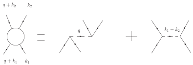
Figure 1: Direct and exchange parts of the p-h interaction.

In the HF approximation, the p-h Green function does not depend on the spin-isospin channel $(\alpha)$ and reads Fetter and Walecka (1971)

$$G_{HF}(q,\omega,{\bf k}_{1})=\frac{\theta(k_{F}-k_{1})-\theta(k_{F}-|{\bf k}_{1}+{\bf q}|)}{\omega+\varepsilon(k_{1})-\varepsilon(|{\bf k}_{1}+{\bf q}|)+i\eta\omega}\,.$$ (5)

To go beyond the HF approximation one takes into account long-range correlations by resumming a class of p-h diagrams to obtain the well-known Random Phase Approximation Fetter and Walecka (1971). The interaction appearing in the RPA is the p-h residual interaction whose matrix element including the exchange part can be written as

$$V_{ph}^{(\alpha,\alpha^{\prime})}(q,{\bf k}_{1},{\bf k}_{2})\equiv\langle\,{\bf q}+{\bf k}_{1},{\bf k}_{1}^{\text{-}1},(\alpha)|V|{\bf q}+{\bf k}_{2},{\bf k}_{2}^{\text{-}1},(\alpha^{\prime})\,\rangle\,.$$ (6)

In the general case, the residual interaction is obtained by taking the second derivative of the total energy with respect to the densities built from the Hartree-Fock solutions. In the absence of density dependent terms, it can also be obtained by standard techniques of particle-hole configuration Brussaard and Glaudemans (1977).

The first important step is thus to determine the matrix elements for the different parts of the p-h interaction from eqs. (II), (3) and (4).

III.1 The particle-hole interaction

III.1.1 Central part of the force

The central component of the p-h interaction can be written in the general form

$$V_{\mathrm{C},ph}^{(\alpha,\alpha^{\prime})}(q,{\bf k}_{1},{\bf k}_{2})=\delta_{\alpha\alpha^{\prime}}\left\{W^{(\alpha)}_{1}+W^{(\alpha)}_{2}\left[k_{1}^{2}+k_{2}^{2}\right]-W^{(\alpha)}_{2}\frac{8\pi}{3}k_{1}k_{2}\sum_{\mu=0,\pm 1}Y^{(1)\,*}_{\mu}(\hat{k}_{1})Y^{(1)}_{\mu}(\hat{k}_{2})\right\}\,,$$ (7)

where the $W^{(\alpha)}_{1}$ and $W^{(\alpha)}_{2}$ coefficients are functions of the Skyrme parameters $(t_{i},x_{i})$ and of the transferred momentum ${\bf q}$ represented on figure 1. Their detailed expressions have been given by Garcia-Recio et al. Garcia-Recio et al. (1992) and Navarro et al. Navarro et al. (1999) for the symmetric nuclear matter and pure neutron matter respectively while Hernandez et al. Hernandez et al. (1997) gave them for an arbitrary neutron-proton asymmetry. The case of symmetric nuclear matter studied here is recalled in the Appendix B. The central part of the Skyrme interaction being usually density dependent, it is not trivialy related to the p-h interaction since the $W^{(\alpha)}_{i}$ coefficients contain rearrangement terms. One can note at this level, using only the central part of the interaction, that there is no coupling between the different spin and isospin channels.

III.1.2 Spin-orbit part of the force

To calculate the contribution of the spin-orbit term (see eq. (3)) to the p-h interaction one has to evaluate the matrix element of the spin-orbit interaction. Since this term is density-independent there is no rearrangement contribution and the result is just adding the following term to eq. (7) (see Margueron et al. Margueron et al. (2006)):

$$V_{\mathrm{LS},ph}^{(\alpha,\alpha^{\prime})}(q, {\bf k}_{1},{\bf k}_{2})=-\delta_{II^{\prime}}\,w(I)\,\sqrt{\frac{4\pi}{3}}\,q\,W_{0}\,$$ (8)

$$\times\bigg{\{} \delta_{S1}\delta_{S^{\prime}0}M\left[k_{1}Y^{(1)}_{\text{-}M}(\hat{k}_{1})-k_{2}Y^{(1)}_{\text{-}M}(\hat{k}_{2})\right]$$

$$+ \,\delta_{S0}\delta_{S^{\prime}1}M^{\prime}\left[k_{1}Y^{(1)}_{M^{\prime}}(\hat{k}_{1})-k_{2}Y^{(1)}_{M^{\prime}}(\hat{k}_{2})\right]\bigg{\}}~{},$$

the factor $w(I)=3$ for $I=0$ and $w(I)=1$ for $I=1$ in the case of symmetric nuclear matter. It is clear from this expression that the main effect of the spin-orbit component is to couple the $S=0$ and $S=1$ channels.

III.1.3 Tensor part of the force

With the tensor force previously defined (see eq. (4)), we have to calculate the antisymmetrized particle-hole matrix elements $\langle\,IQSM;ph\,|v_{\mathrm{T}}|\,I^{\prime}Q^{\prime}S^{\prime}M^{\prime};ph\,\rangle$. Their analytical expressions are summarized in Table 2 where we have adopted the following notation:

$$(k_{12})^{(1)}_{M}\equiv\sqrt{\frac{4\pi}{3}}\left[k_{1}Y^{(1)}_{M}(\hat{k}_{1})-k_{2}Y^{(1)}_{M}(\hat{k}_{2})\right]\,.$$ (9)

Even if one can note from Table 2 that channels with different spin projection $M$ are now coupled in a non trivial way, these additional matrix elements are still diagonal in isospin space and act only in the vector channel. However, since we include both spin-orbit and tensor interactions in our approach, it is fundamental to note that the tensor component will impact both scalar and vector channels via the spin-orbit term.

III.2 Response function

With the particle-hole matrix elements we are now in position to solve the RPA problem itself, that is the Bethe-Salpeter equation satisfied by the RPA correlated Green function $G_{RPA}^{(\alpha)}(q,\omega,{\bf k}_{1})$:

$$G_{RPA}^{(\alpha)}(q,\omega,{\bf k}_{1}) = G_{HF}(q,\omega,{\bf k}_{1})+G_{HF}(q,\omega,{\bf k}_{1})\,$$ (10)

$$\times\sum_{(\alpha^{\prime})}\,\int\frac{{\mathrm{d}}^{3}k_{2}}{(2\pi)^{3}}\,V_{ph}^{(\alpha,\alpha^{\prime})}(q,{\bf k}_{1},{\bf k}_{2})$$

$$\times\,G_{RPA}^{(\alpha^{\prime})}(q,\omega,{\bf k}_{2})\,.$$

The response function $\chi^{(\alpha)}(q,\omega)$ in the infinite medium is related to the p-h Green function by:

$$\chi_{RPA}^{(\alpha)}(q,\omega)\,=\,g\int\frac{{\mathrm{d}}^{3}k_{1}}{(2\pi)^{3}}\,G_{RPA}^{(\alpha)}(q,\omega,{\bf k}_{1})~{},$$ (11)

where the spin-isospin degeneracy factor $g$ is 4 for symmetric nuclear matter. The Lindhard function $\chi_{HF}$ is obtained when the free p-h propagator $G_{HF}$ is used in eq. (11).

Following the notation of refs.Garcia-Recio et al. (1992); Margueron et al. (2006), we define for any function $f(q,\omega,k_{1})$:

$$\langle\,f(\mathbf{k}_{1})\,\rangle\,\equiv\,\int\frac{\mathrm{d}^{3}{\bf k}_{1}}{(2\pi)^{3}}\,f(k_{1})\,.$$ (12)

The response function can thus be written in each channel $(\alpha)$ as:

$$\chi_{RPA}^{(\alpha)}\,=\,g\,\langle\,G_{RPA}^{(\alpha)}\,\rangle\,.$$ (13)

Finally, the quantity of interest is the dynamical structure function $S^{(\alpha)}(q,\omega)$ which is, at zero temperature, proportional to the imaginary part of the response function at positive energies:

$$S^{(\alpha)}(q,\omega)=-\frac{1}{\pi}\,\rm{Im}\,\chi_{RPA}^{(\alpha)}(q,\omega)\,.$$ (14)

III.3 Response function for the spin-orbit case

As an introduction to our full calculation we recall here some results already obtained by Margueron et al. Margueron et al. (2006). When the spin-orbit force alone is included, the response function can then be written in the form (using $\hbar=c=1$):

$$\frac{\chi_{HF}}{\chi^{(\alpha)}_{RPA}} = 1-{\widetilde{W}}^{(\alpha)}_{1}\chi_{0}+W^{(\alpha)}_{2}\left[\frac{q^{2}}{2}\chi_{0}-2k_{F}^{2}\chi_{2}\right]$$

$$+ \left[W^{(\alpha)}_{2}k_{F}^{2}\right]^{2}\left[\chi_{2}^{2}-\chi_{0}\chi_{4}+\left(\frac{m^{*}\omega}{k_{F}^{2}}\right)^{2}\chi_{0}^{2}-\frac{m^{*}}{6\pi^{2}k_{F}}q^{2}\chi_{0}\right]+2\left(\frac{m^{*}\omega}{q}\right)^{2}\frac{W^{(\alpha)}_{2}}{1-\frac{m^{*}k_{F}^{3}}{3\pi^{2}}W^{(\alpha)}_{2}}\chi_{0}\,.$$

In this expression $k_{F}$ is the Fermi momentum whereas $m^{*}$ denotes the effective mass of the nucleons. The functions $\chi_{0}$, $\chi_{2}$ and $\chi_{4}$ are generalized free response functions, defined in ref.Garcia-Recio et al. (1992) and written in Appendix D, see eq. (37), and $\chi_{HF}=g\,\chi_{0}$.

The explicit expressions of the ${\widetilde{W}}^{(\alpha)}_{1}$ coefficients are given in Appendix C where the coupling between the $S=0$ and $S=1$ channels induced by the spin-orbit interaction can also be clearly seen. It can be noted that the coefficients ${\widetilde{W}}^{(\alpha)}_{1}$ are now complex functions of $q$ and $\omega$ since different moments $\chi_{2i}$ enter their expressions. If we replace ${\widetilde{W}}^{(\alpha)}_{1}$ in eq. (III.3) by $W^{(\alpha)}_{1}$ we obtain the results of ref.Garcia-Recio et al. (1992), related to the central part of the interaction, as it should be.

III.4 Response function with the tensor part

As already mentioned, the tensor interaction couples vector channels with different spin projection while the spin-orbit interaction couples the scalar ($S=0$) and vector ($S=1$) ones. The consequence is that we obtain a non trivial system of coupled equations for the RPA problem. As an illustration let us consider explicitly the case of isospin $I=0$ and $(S,M)=(1,1)$. In that particular channel, the Bethe-Salpeter equation for $G_{RPA}^{(1,1)}(k_{1})$ (we omit the isospin index and dependence on $q$ and $\omega$ for sake of simplicity) exhibits terms which typically read:

• $G_{HF}(k_{1})\langle\,G_{RPA}^{(1,1)}\,\rangle$ ,

• $G_{HF}(k_{1})\langle\,k^{2}G_{RPA}^{(1,1)}\,\rangle$ ,

• $k_{1}Y^{(1)*}_{\mu}G_{HF}(k_{1})\langle\,kY^{(1)}_{\mu}G_{RPA}^{(1,1)}\,\rangle$ ,

• $k_{1}Y^{(1)}_{\text{-}1}G_{HF}(k_{1})\langle\,G_{RPA}^{(1,0)}\,\rangle$ ,

• $G_{HF}(k_{1})\langle\,k^{2}Y^{(1)}_{\text{-}1}Y^{(1)}_{\text{-}1}G_{RPA}^{(1,\,\text{-}1)}\,\rangle$ .

Thus, the determination of $\langle\,G_{RPA}^{(1,1)}\,\rangle$ requires the knowledge of some other unknown quantities. This leads to a large system of coupled equations for:

• $\langle\,G_{RPA}^{(1,M)}\,\rangle$ ,

• $\langle\,k^{2}G_{RPA}^{(1,M)}\,\rangle$ ,

• $\langle\,kY^{(1)}_{0}G_{RPA}^{(1,M)}\,\rangle$ ,

• $\langle\,k^{2}|Y^{(1)}_{0}|^{2}G_{RPA}^{(1,M)}\,\rangle$ ,

• $\langle\,k^{2}|Y^{(1)}_{1}|^{2}G_{RPA}^{(1,M)}\,\rangle$ for $M=-1,0,1$ ,

and

• $\langle\,k^{2}Y^{(1)}_{1}Y^{(1)}_{1}G_{RPA}^{(1,1)}\,\rangle$ ,

• $\langle\,k^{2}Y^{(1)}_{\text{-}1}Y^{(1)}_{\text{-}1}G_{RPA}^{(1,\,\text{-}1)}\,\rangle$ ,

• $\langle\,kY^{(1)}_{1}G_{RPA}^{(1,1)}\,\rangle$ ,

• $\langle\,kY^{(1)}_{\text{-}1}G_{RPA}^{(1,\,\text{-}1)}\,\rangle$ ,

• $\langle\,kY^{(1)}_{1}G_{RPA}^{(1,0)}\,\rangle$ ,

• $\langle\,kY^{(1)}_{\text{-}1}G_{RPA}^{(1,0)}\,\rangle$ ,

that is 21 unknown quantities. Fortunately, since the multipole expansion of $G_{HF}$ only implies terms with $Y^{(L)}_{0}$, the integration over $k_{1}$ cancels all terms of the form $\langle\,f(k)\prod_{\{M,M^{\prime},...\}}Y^{(1)}_{M}Y^{(1)}_{M^{\prime}}...G_{HF}\,\rangle$ with $M+M^{\prime}+...\neq 0$. Moreover some unknown quantities can be expressed through the others and we can reduce the 21 coupled equations to three systems of four coupled equations for the following variables:

$$\langle\,G_{RPA}^{(1,M)}\,\rangle\,,~{}~{}~{}\langle\,k^{2}G_{RPA}^{(1,M)}\,\rangle\,,~{}~{}~{}\langle\,kY^{(1)}_{0}G_{RPA}^{(1,M)}\,\rangle\,,~{}~{}~{}$$

$$\langle\,k^{2}|Y^{(1)}_{0}|^{2}G_{RPA}^{(1,M)}\,\rangle-\langle\,k^{2}|Y^{(1)}_{1}|^{2}G_{RPA}^{(1,M)}\,\rangle\,,$$

for each value of $M$. The calculations are straightforward but tedious. The same procedure has to be repeated for isospin $I=1$ for $S=1$. Indeed, only the channels with $S=0$ are less involved.

The results are now quoted for each spin-isospin channel in a form that exhibits the symmetry properties appearing in Table 2:

• For $S=0,I=0$:

  $$\frac{\chi_{HF}}{\chi^{(0,0)}_{RPA}} = \,1\,-\,{\widetilde{\widetilde{W}}}^{(0,0)}_{1}\chi_{0}\,+\,W^{(0,0)}_{2}\left(\frac{q^{2}}{2}\chi_{0}-2k_{F}^{2}\chi_{2}\right)\,+\,\left[W^{(0,0)}_{2}k_{F}^{2}\right]^{2}\left[\chi_{2}^{2}-\chi_{0}\chi_{4}+\left(\frac{m^{*}\omega}{k_{F}^{2}}\right)^{2}\chi_{0}^{2}-\frac{m^{*}}{6\pi^{2}k_{F}}q^{2}\chi_{0}\right]$$ (16)

  $$+ \,2\chi_{0}\left(\frac{m^{*}\omega}{q}\right)^{2}\frac{W^{(0,0)}_{2}}{1-\frac{m^{*}k_{F}^{3}}{3\pi^{2}}W^{(0,0)}_{2}}\,.$$

• For $S=0,I=1$:

  $$\frac{\chi_{HF}}{\chi^{(0,1)}_{RPA}} = \,1\,-\,{\widetilde{\widetilde{W}}}^{(0,1)}_{1}\chi_{0}\,+\,W^{(0,1)}_{2}\left(\frac{q^{2}}{2}\chi_{0}-2k_{F}^{2}\chi_{2}\right)\,+\,\left[W^{(0,1)}_{2}k_{F}^{2}\right]^{2}\left[\chi_{2}^{2}-\chi_{0}\chi_{4}+\left(\frac{m^{*}\omega}{k_{F}^{2}}\right)^{2}\chi_{0}^{2}-\frac{m^{*}}{6\pi^{2}k_{F}}q^{2}\chi_{0}\right]$$ (17)

  $$+ \,2\chi_{0}\left(\frac{m^{*}\omega}{q}\right)^{2}\frac{W^{(0,1)}_{2}}{1-\frac{m^{*}k_{F}^{3}}{3\pi^{2}}W^{(0,1)}_{2}}\,.$$

• For $S=1,I=0,M=\pm 1$:

  $$\frac{\chi_{HF}}{\chi^{(1,0,\pm 1)}_{RPA}} = \,\left[1+(t_{e}-5t_{o})\frac{m^{*}k_{F}^{3}}{2\pi^{2}}\right]^{2}\,-\,{\widetilde{\widetilde{W}}}^{(1,0,\pm 1)}_{1}\chi_{0}$$

  $$+ \,\left[W^{(1,0)}_{2}-(t_{e}-5t_{o})\right]\left\{\frac{q^{2}}{2}\chi_{0}\left[1+(t_{e}-5t_{o})\frac{m^{*}k_{F}^{3}}{\pi^{2}}\right]-2k_{F}^{2}\chi_{2}+(t_{e}-5t_{o})\frac{m^{*}k_{F}^{5}}{\pi^{2}}\left(\chi_{0}-\chi_{2}\right)\right\}$$

  $$+ \,\left[W^{(1,0)}_{2}-(t_{e}-5t_{o})\right]^{2}k_{F}^{4}\left[\chi_{2}^{2}-\chi_{0}\chi_{4}+\left(\frac{m^{*}\omega}{k_{F}^{2}}\right)^{2}\chi_{0}^{2}-\frac{m^{*}}{6\pi^{2}k_{F}}q^{2}\chi_{0}\right]$$

  $$+ \,2\left(\frac{m^{*}\omega}{q}\right)^{2}\frac{W^{(1,0)}_{2}+2(t_{e}-5t_{o})+X^{(1,0,\pm 1)}}{1-\frac{m^{*}k_{F}^{3}}{3\pi^{2}}\left[W^{(1,0)}_{2}+2(t_{e}-5t_{o})-X^{(1,0,\pm 1)}\right]}\,\chi_{0}$$

  $$+ \left\{2m^{*}\omega X^{(1,0,\pm 1)}+\frac{2m^{*}k_{F}^{3}}{3\pi^{2}}\left[X^{(1,0,\pm 1)}\right]^{2}\left[\frac{q}{2}+\frac{m^{*}\omega}{q}\right]^{2}\right\}\frac{\chi_{0}}{1-\frac{m^{*}k_{F}^{3}}{3\pi^{2}}\left[W^{(1,0)}_{2}+2(t_{e}-5t_{o})-X^{(1,0,\pm 1)}\right]}\,.$$

• For $S=1,I=0,M=0$:

  $$\frac{\chi_{HF}}{\chi^{(1,0,0)}_{RPA}} = \,\left[1-\tfrac{1}{2}(t_{e}-5t_{o})\frac{m^{*}k_{F}^{3}}{2\pi^{2}}\right]^{2}\,-\,{\widetilde{\widetilde{W}}}^{(1,0,0)}_{1}\chi_{0}$$

  $$+ \,\left[W^{(1,0)}_{2}+\tfrac{1}{2}(t_{e}-5t_{o})\right]\left\{\frac{q^{2}}{2}\chi_{0}\left[1-(t_{e}-5t_{o})\frac{m^{*}k_{F}^{3}}{2\pi^{2}}\right]-2k_{F}^{2}\chi_{2}-(t_{e}-5t_{o})\frac{m^{*}k_{F}^{5}}{2\pi^{2}}\left(\chi_{0}-\chi_{2}\right)\right\}$$

  $$+ \,\left[W^{(1,0)}_{2}+\tfrac{1}{2}(t_{e}-5t_{o})\right]^{2}k_{F}^{4}\left[\chi_{2}^{2}-\chi_{0}\chi_{4}+\left(\frac{m^{*}\omega}{k_{F}^{2}}\right)^{2}\chi_{0}^{2}-\frac{m^{*}}{6\pi^{2}k_{F}}q^{2}\chi_{0}\right]$$

  $$+ \,2\left(\frac{m^{*}\omega}{q}\right)^{2}\frac{W^{(1,0)}_{2}-(t_{e}-5t_{o})+X^{(1,0,0)}}{1-\frac{m^{*}k_{F}^{3}}{3\pi^{2}}[W^{(1,0)}_{2}-(t_{e}-5t_{o})-X^{(1,0,0)}]}\,\chi_{0}$$

  $$+ \,\left\{-2m^{*}\omega X^{(1,0,0)}+\frac{2m^{*}k_{F}^{3}}{3\pi^{2}}\left[X^{(1,0,0)}\right]^{2}\left[\frac{q}{2}-\frac{m^{*}\omega}{q}\right]^{2}\right\}\frac{\chi_{0}}{1-\frac{m^{*}k_{F}^{3}}{3\pi^{2}}[W^{(1,0)}_{2}-(t_{e}-5t_{o})-X^{(1,0,0)}]}\,.$$

• For $S=1,I=1,M=\pm 1$:

  $$\frac{\chi_{HF}}{\chi^{(1,1,\pm 1)}_{RPA}} = \,\left[1+3(t_{e}-t_{o})\frac{m^{*}k_{F}^{3}}{2\pi^{2}}\right]^{2}\,-\,{\widetilde{\widetilde{W}}}^{(1,1,\pm 1)}_{1}\chi_{0}$$

  $$+ \,\left[W^{(1,1)}_{2}-3(t_{e}-t_{o})\right]\left\{\frac{q^{2}}{2}\chi_{0}\left[1+3(t_{e}-t_{o})\frac{m^{*}k_{F}^{3}}{\pi^{2}}\right]-2k_{F}^{2}\chi_{2}+3(t_{e}-t_{o})\frac{m^{*}k_{F}^{5}}{\pi^{2}}\left(\chi_{0}-\chi_{2}\right)\right\}$$

  $$+ \,\left[W^{(1,1)}_{2}-3(t_{e}-t_{o})\right]^{2}k_{F}^{4}\left[\chi_{2}^{2}-\chi_{0}\chi_{4}+\left(\frac{m^{*}\omega}{k_{F}^{2}}\right)^{2}\chi_{0}^{2}-\frac{m^{*}}{6\pi^{2}k_{F}}q^{2}\chi_{0}\right]$$

  $$+ \,2\left(\frac{m^{*}\omega}{q}\right)^{2}\frac{W^{(1,1)}_{2}+6(t_{e}-t_{o})+X^{(1,1,\pm 1)}}{1-\frac{m^{*}k_{F}^{3}}{3\pi^{2}}[W^{(1,1)}_{2}+6(t_{e}-t_{o})-X^{(1,1,\pm 1)}]}\,\chi_{0}$$

  $$+ \,2\left(\frac{m^{*}\omega}{q}\right)^{2}\frac{m^{*}k_{F}^{3}}{3\pi^{2}}\left[X^{(1,1,\pm 1)}\right]^{2}\frac{\chi_{0}}{1-\frac{m^{*}k_{F}^{3}}{3\pi^{2}}[W^{(1,1)}_{2}+6(t_{e}-t_{o})-X^{(1,1,\pm 1)}]}\,.$$

• For $S=1,I=1,M=0$:

  $$\frac{\chi_{HF}}{\chi^{(1,1,0)}_{RPA}} = \,\left[1-\tfrac{3}{2}(t_{e}-t_{o})\frac{m^{*}k_{F}^{3}}{2\pi^{2}}\right]^{2}\,-\,{\widetilde{\widetilde{W}}}^{(1,1,0)}_{1}\chi_{0}$$

  $$+ \left[W^{(1,1)}_{2}+\tfrac{3}{2}(t_{e}-t_{o})\right]\left\{\frac{q^{2}}{2}\chi_{0}\left[1-3(t_{e}-t_{o})\frac{m^{*}k_{F}^{3}}{2\pi^{2}}\right]-2k_{F}^{2}\chi_{2}-\tfrac{3}{2}(t_{e}-t_{o})\frac{m^{*}k_{F}^{5}}{\pi^{2}}\left(\chi_{0}-\chi_{2}\right)\right\}$$

  $$+ \,\left[W^{(1,1)}_{2}+\tfrac{3}{2}(t_{e}-t_{o})\right]^{2}k_{F}^{4}\left[\chi_{2}^{2}-\chi_{0}\chi_{4}+\left(\frac{m^{*}\omega}{k_{F}^{2}}\right)^{2}\chi_{0}^{2}-\frac{m^{*}}{6\pi^{2}k_{F}}q^{2}\chi_{0}\right]$$

  $$+ \,2\left(\frac{m^{*}\omega}{q}\right)^{2}\frac{W^{(1,1)}_{2}-3(t_{e}-t_{o})+X^{(1,1,0)}}{1-\frac{m^{*}k_{F}^{3}}{3\pi^{2}}[W^{(1,1)}_{2}-3(t_{e}-t_{o})-X^{(1,1,0)}]}\chi_{0}$$

  $$+ \,2\left(\frac{m^{*}\omega}{q}\right)^{2}\frac{m^{*}k_{F}^{3}}{3\pi^{2}}\left[X^{(1,1,0)}\right]^{2}\frac{\chi_{0}}{1-\frac{m^{*}k_{F}^{3}}{3\pi^{2}}[W^{(1,1)}_{2}-3(t_{e}-t_{o})-X^{(1,1,0)}]}\,.$$

The coefficients ${\widetilde{\widetilde{W}}}^{(S,I)}_{1}$ for $S=0$ or ${\widetilde{\widetilde{W}}}^{(S,I,M)}_{1}$ for $S=1$ are defined as

$${\widetilde{\widetilde{W}}}^{(0,0)}_{1}\, = \,W^{(0,0)}_{1}\,+\,9W_{0}^{2}q^{4}\frac{\beta_{2}-\beta_{3}}{1+q^{2}(\beta_{2}-\beta_{3})(W^{(1,0)}_{2}-(7t_{e}+13t_{o}))}$$ (22)

$${\widetilde{\widetilde{W}}}^{(0,1)}_{1}\, = \,W^{(0,1)}_{1}\,+\,W_{0}^{2}q^{4}\frac{\beta_{2}-\beta_{3}}{1+q^{2}(\beta_{2}-\beta_{3})[W^{(1,1)}_{2}+3(t_{e}-t_{o})]}$$ (23)

$${\widetilde{\widetilde{W}}}^{(1,0,\pm 1)}_{1}\, = \,{\widetilde{W}}^{(1,0,\pm 1)}_{1}+K_{1}+K_{2}-\,t_{o}^{2}\,\frac{24m^{*}k_{F}^{5}}{5\pi^{2}}$$ (24)

$$+ \,9(t_{e}+3t_{o})^{2}q^{4}(\beta_{5}-2\beta_{8}+\beta_{7})+2X^{(1,0,\pm 1)}\left[\frac{q}{2}+\frac{m^{*}\omega}{q}\right]^{2}$$

$${\widetilde{\widetilde{W}}}^{(1,0,0)}_{1}\, = \,{\widetilde{W}}^{(1,0,0)}_{1}-\tfrac{1}{2}K_{1}+\tfrac{1}{4}K_{2}-\,t_{o}^{2}\frac{48m^{*}k_{F}^{5}}{5\pi^{2}}+2X^{(1,0,0)}\left[\frac{q}{2}-\frac{m^{*}\omega}{q}\right]^{2}$$ (25)

$${\widetilde{\widetilde{W}}}^{(1,1,\pm 1)}_{1}\, = \,{\widetilde{W}}^{(1,1,\pm 1)}_{1}+3K^{\prime}_{1}+9K^{\prime}_{2}-\,(t_{e}-t_{o})^{2}\frac{6m^{*}k_{F}^{5}}{5\pi^{2}}$$ (26)

$$+ \,9(t_{e}-t_{o})^{2}q^{4}(\beta_{5}-2\beta_{8}+\beta_{7})+2X^{(1,1,\pm 1)}\left(\frac{m^{*}\omega}{q}\right)^{2}$$

$${\widetilde{\widetilde{W}}}^{(1,1,0)}_{1}\, = \,{\widetilde{W}}^{(1,1,0)}_{1}-\tfrac{3}{2}K^{\prime}_{1}+\tfrac{9}{4}K^{\prime}_{2}-\,(t_{e}-t_{o})^{2}\frac{12m^{*}k_{F}^{5}}{5\pi^{2}}+2X^{(1,1,0)}\left(\frac{m^{*}\omega}{q}\right)^{2}\,.$$ (27)

The functions $\beta_{i}$ are given in Appendix D and the coefficients $K_{i}$, $K_{i}^{\prime}$ and $X^{(S,I,M)}$ are

$$K_{1} = 2(t_{e}+5t_{o})q^{2}+6\left(\frac{m^{*}\omega}{q}\right)^{2}(t_{e}-5t_{o})\,,$$ (28)

$$K_{2} = -(t_{e}-5t_{o})^{2}\,\frac{m^{*}k_{F}^{3}}{\pi^{2}}\left[\frac{9}{10}k_{F}^{2}+\frac{3}{8}q^{2}-\frac{3}{2}\left(\frac{m^{*}\omega}{q}\right)^{2}\right]\,,$$ (29)

$$K^{\prime}_{1} = 2(t_{e}+t_{o})q^{2}+6\left(\frac{m^{*}\omega}{q}\right)^{2}(t_{e}-t_{o})\,,$$ (30)

$$K^{\prime}_{2} = -(t_{e}-t_{o})^{2}\,\frac{m^{*}k_{F}^{3}}{\pi^{2}}\left[\frac{9}{10}k_{F}^{2}+\frac{3}{8}q^{2}-\frac{3}{2}\left(\frac{m^{*}\omega}{q}\right)^{2}\right]\,,$$ (31)

and

$$X^{(1,0,\pm 1)}\, = \,36t_{o}^{2}q^{2}\frac{\beta_{2}-\beta_{3}}{1+q^{2}(\beta_{2}-\beta_{3})(W^{(1,0)}_{2}+\tfrac{1}{2}(t_{e}-5t_{o}))}\,,$$ (32)

$$X^{(1,0,0)}\, = \,72t_{o}^{2}q^{2}\frac{\beta_{2}-\beta_{3}}{1+q^{2}(\beta_{2}-\beta_{3})(W^{(1,0)}_{2}+5t_{e}+23t_{o})}\,,$$ (33)

$$X^{(1,1,\pm 1)}\, = \,9(t_{e}-t_{o})^{2}q^{2}\frac{\beta_{2}-\beta_{3}}{1+q^{2}(\beta_{2}-\beta_{3})(W^{(1,1)}_{2}+\tfrac{3}{2}(t_{e}-t_{o}))}\,,$$ (34)

$$X^{(1,1,0)}\, = \,18(t_{e}-t_{o})^{2}q^{2}\frac{\beta_{2}-\beta_{3}}{1+q^{2}(\beta_{2}-\beta_{3})(W^{(1,1)}_{2}-9(t_{e}-t_{o}))}\,.$$ (35)

It is important to note that the above response functions have exactly the same structure as in HF, with or without the spin-orbit interaction. Moreover we can see that the response function depends on different linear combinations of the parameters $t_{e}$ and $t_{o}$ that will lead to non trivial effects.

IV Dynamical structure function with tensor contribution

As an example for the effect of a zero-range tensor force in the p-h interaction, we have calculated the nuclear responses in $(S,I,M)$ channels of symmetric infinite nuclear matter for parametrization T44 of the Skyrme interaction built by Lesinski et al. Lesinski et al. (2007). The parameters of this force are given in Table 1. The dynamical structure functions $S^{(\alpha)}(\mathrm{q},\omega)$ (defined in eq. (14)) calculated for $q=k_{F}$ and at the saturation density $\rho=\rho_{\mathrm{sat}}=0.16~{}\mathrm{fm}^{-3}$ are shown on Figure 2. To clearly isolate the effect of the tensor part of the force, the functions $S^{(\alpha)}(\mathrm{q},\omega)$ are plotted for two cases: a) with no tensor contribution but including the spin-orbit part; b) with the full force. The first case allows to compare with the previous results of Margueron et al. Margueron et al. (2006) but are presented here for the four channels of the symmetric nuclear matter.

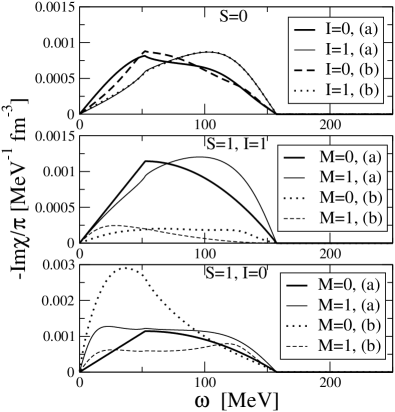
Figure 2: Dynamical structure functions $S^{(\alpha)}(\mathrm{q},\omega)$ calculated for the Skyrme tensor parametrization T44 Lesinski et al. (2007). The upper (middle and lower respectively) part of the Figure concerns the channels $S=0$, $S=1$ and $I=0$, $S=1$ and $I=0$. For each $(S,I,M)$ channel the responses (in MeV^-1 fm^-3) are plotted as a function of $\omega$ (in MeV). All the responses are calculated for $q=k_{F}$ at saturation density. Cases (a) and (b) are discussed in the text.

$t_{0}$	$x_{0}$	$t_{1}$	$x_{1}$	$t_{2}$	$x_{2}$
-2485.67	0.721557	494.477	-0.661848	-337.961	-0.803184
$t_{3}$	$x_{3}$	$\gamma$	$W_{0}$	$t_{e}$	$t_{o}$
13794.7	1.175908	1/6	161.367	173.661	7.17383

Table 1: Parameters of the interaction T44 Lesinski et al. (2007) as defined in equations (II), (3) and (4).

In $S=0$ channel, the tensor terms do not affect qualitatively the response. Strictly speaking, this comment only applies to the case of the T44 tensor parametrization but several tests performed using other Tij tensor interactions discussed in ref.Lesinski et al. (2007) exhibit the same qualitative behaviour. The situation is quite different in $S=1$ channels: the effect from the tensor terms is large whatever the value of the spin projection $M$ is. Actually, depending on the values of the transferred momentum $q$ and the density $\rho$, the response functions increase significantly and diverge at finite $q$ for a certain critical density $\rho_{c}$. This divergence reveals the presence of instabilities observed in nuclei Lesinski et al. (2006), with the appearance of domains with typical size of the order of $2\pi/q$. Even if a one-to-one correspondence between infinite matter and finite nuclei is obviously not correct, it remains that the center of a nucleus explores, because of fluctuations, not only the saturation density but also some larger values for which one may observe a divergence of the response functions, and then, possibly, the appearance of finite-size instabilities in the nucleus.

V Summary and conclusions

We have derived the contribution from the tensor terms in the Skyrme effective interaction to the RPA response function. We have shown that the formal structure of the response function is the same as without tensor terms, although with the latter, all channels are coupled in a non trivial way. The simple example presented here, using the interaction T44, shows that the effects of the tensor contributions are strong in vector channels.

We have shown that the dynamical structure functions $S^{(\alpha)}(q,\omega)$ becomes large for finite values of $q$. This indicates the vicinity of a pole related with a finite size instability for given values of $q$ and $\rho$ in infinite matter and, possibly, in finite nuclei. A systematic study of the critical densities is in progress in order to determine if the link between the divergences of $\chi_{RPA}$ and the instabilities encountered in nuclei at the Hartree-Fock approximation is robust.

Another important point under study is the identification, directly from the Skyrme energy functional, of the origin of each tensorial contribution in the response functions. In the same spirit, a detailed study of sum rules can enlighten the contribution of the tensor for various physical situations (see Lipparini and Stringari (1989)). Finally, applications to pure neutron matter can be very important (see by instance Marcos et al. (1991); Fantoni et al. (2001); Margueron et al. (2002); Vidana et al. (2002); Vidana and Bombaci (2002); Margueron and Sagawa (2009); Isayev and Yang (2004); Beraudo et al. (2004, 2005); Rios et al. (2005); Lopez-Val et al. (2006); Krastev and Sammarruca (2007); Bordbar and Bigdeli (2008)). However, above formulae are no longer directly usable and have to be adapted to that specific case. Work in that direction is also in progress.

Appendix A Coupling constants of the Skyrme energy functional

The Skyrme energy density functional used in this article is a functional of local densities and currents (with $q=n,\,p$ for neutrons and protons), i.e. the particle densities $\rho_{q}({\mathbf{r}})$, the kinetic densities $\tau_{q}({\mathbf{r}})$, the current (vector) densities ${\mathbf{j}}_{q}({\mathbf{r}})$, the spin (pseudovector) densities ${\mathbf{s}}_{q}({\mathbf{r}})$, the spin kinetic (pseudovector) densities ${\mathbf{T}}_{q}({\mathbf{r}})$, the spin-current (pseudotensor) densities $J_{q,\mu\nu}({\mathbf{r}})$ and the tensor-kinetic (pseudovector) densities ${\mathbf{F}}_{q}({\mathbf{r}})$ that have been defined in Lesinski et al. Lesinski et al. (2007), where the definition of the vector spin current density ${\mathbf{J}}^{(1)}({\mathbf{r}})\equiv{\mathbf{J}}({\mathbf{r}})$ was also recalled. We will use also the isoscalar and isovector densities defined from the proton and neutron densities respectively as: $\rho_{0}({\mathbf{r}})=\rho_{\mathrm{n}}({\mathbf{r}})+\rho_{\mathrm{p}}({\mathbf{r}})$ and $\rho_{1}({\mathbf{r}})=\rho_{\mathrm{n}}({\mathbf{r}})-\rho_{\mathrm{p}}({\mathbf{r}})$, and similar for all other densities.

The Skyrme energy functional representing central, tensor and spin-orbit contributions is given by:

$$\mathcal{E}_{\text{Skyrme}} = \mathcal{E}_{\mathrm{C}}+\mathcal{E}_{\mathrm{LS}}+\mathcal{E}_{\mathrm{T}}$$

$$= \int\!\mathrm{d}^{3}\mathbf{r}\sum_{t=0,1}\bigg{\{}\,C^{\rho}_{t}[\rho_{0}]\,\rho_{t}^{2}\,+\,C^{\Delta\rho}_{t}\,\rho_{t}\Delta\rho_{t}\,+\,C^{\tau}_{t}\,(\rho_{t}\tau_{t}-{\mathbf{j}}_{t}^{2})$$

$$\,+\,C^{s}_{t}[\rho_{0}]\,{\mathbf{s}}_{t}^{2}\,+\,C^{\nabla s}_{t}\,\left(\boldsymbol{\nabla}\cdot{\mathbf{s}}_{t}\right)^{2}\,+\,C^{\Delta s}_{t}\,{\mathbf{s}}_{t}\cdot\Delta{\mathbf{s}}_{t}$$

$$\,+\,C^{T}_{t}\Big{(}{\mathbf{s}}_{t}\cdot{\mathbf{T}}_{t}-\sum_{\mu,\nu=x}^{z}J_{t,\mu\nu}J_{t,\mu\nu}\Big{)}\,+\,C^{F}_{t}\Big{[}{\mathbf{s}}_{t}\cdot{\mathbf{F}}_{t}-\tfrac{1}{2}\Big{(}\sum_{\mu=x}^{z}J_{t,\mu\mu}\Big{)}^{2}-\tfrac{1}{2}\sum_{\mu,\nu=x}^{z}J_{t,\mu\nu}J_{t,\nu\mu}\Big{]}$$

$$\,+\,C^{\nabla J}_{t}\,\big{[}\rho_{t}\boldsymbol{\nabla}\cdot{\mathbf{J}}_{t}+{\mathbf{s}}_{t}\cdot\big{(}\boldsymbol{\nabla}\times{\mathbf{j}}_{t}\big{)}\big{]}\bigg{\}}\,.$$

All the coupling constants can be expressed as function of the parameters of the Skyrme interaction given in eqs. (II), (3) and (4). Some of the coupling constants are fully defined by the standard central part of the Skyrme force: $C^{\rho}_{t}=A^{\rho}_{t}$ , $C^{\Delta\rho}_{t}=A^{\Delta\rho}_{t}$ , $C^{\tau}_{t}=A^{\tau}_{t}$  and $C^{s}_{t}=A^{s}_{t}$ , or by its spin-orbit part: $C^{\nabla J}_{t}=A^{\nabla J}_{t}$, Two coupling constants only depend on the tensor part of the interaction: $C^{\nabla s}_{t}=B^{\nabla s}_{t}$, and $C^{F}_{t}\,=\,B^{F}_{t}$. Finally, two coupling constants are the sum of contributions from both central and tensor forces: $C^{T}_{t}=A^{T}_{t}+B^{T}_{t}$ and $C^{\Delta s}_{t}=A^{\Delta s}_{t}+B^{\Delta s}_{t}$.

The coupling constants of the Skyrme EDF which come from the central and spin-orbit parts of the interaction are given in terms of the parameters by:

$$A_{0}^{\rho}\, = \,\tfrac{3}{8}t_{0}+\tfrac{3}{48}t_{3}\,\rho_{0}^{\gamma}({\mathbf{r}})\,,$$

$$A_{1}^{\rho}\, = \,-\tfrac{1}{4}t_{0}\big{(}\tfrac{1}{2}+x_{0}\big{)}-\tfrac{1}{24}t_{3}\big{(}\tfrac{1}{2}+x_{3}\big{)}\,\rho_{0}^{\gamma}({\mathbf{r}})\,,$$

$$A_{0}^{\Delta\rho}\, = \,-\tfrac{9}{64}t_{1}+\tfrac{1}{16}t_{2}\big{(}\tfrac{5}{4}+x_{2}\big{)}\,,$$

$$A_{1}^{\Delta\rho}\, = \,\tfrac{3}{32}t_{1}\big{(}\tfrac{1}{2}+x_{1}\big{)}+\tfrac{1}{32}t_{2}\big{(}\tfrac{1}{2}+x_{2}\big{)}\,,$$

$$A_{0}^{\tau}\, = \,\tfrac{3}{16}\,t_{1}+\tfrac{1}{4}t_{2}\;\big{(}\tfrac{5}{4}+x_{2}\big{)}\,,$$

$$A_{1}^{\tau}\, = \,-\tfrac{1}{8}t_{1}\big{(}\tfrac{1}{2}+x_{1}\big{)}+\tfrac{1}{8}t_{2}\big{(}\tfrac{1}{2}+x_{2}\big{)}\,,$$

$$A_{0}^{s}\, = \,-\tfrac{1}{4}t_{0}\big{(}\tfrac{1}{2}-x_{0}\big{)}-\tfrac{1}{24}t_{3}\big{(}\tfrac{1}{2}-x_{3}\big{)}\,\rho_{0}^{\gamma}({\mathbf{r}})\,,$$

$$A_{1}^{s}\, = \,-\tfrac{1}{8}t_{0}-\tfrac{1}{48}t_{3}\,\rho_{0}^{\gamma}({\mathbf{r}})\,,$$

$$A_{0}^{\Delta s}\, = \,\tfrac{3}{32}t_{1}\big{(}\tfrac{1}{2}-x_{1}\big{)}+\tfrac{1}{32}t_{2}\big{(}\tfrac{1}{2}+x_{2}\big{)}\,,$$

$$A_{1}^{\Delta s}\, = \,\tfrac{3}{64}t_{1}+\tfrac{1}{64}t_{2}\,,$$

$$A_{0}^{T}\, = \,-\tfrac{1}{8}t_{1}\big{(}\tfrac{1}{2}-x_{1}\big{)}\,+\tfrac{1}{8}t_{2}\big{(}\tfrac{1}{2}+x_{2}\big{)}\,,$$

$$A_{1}^{T}\, = \,-\tfrac{1}{16}t_{1}+\tfrac{1}{16}t_{2}\,,$$

$$A_{0}^{\nabla J}\, = \,-\tfrac{3}{4}\,W_{0}\,,$$

$$A_{1}^{\nabla J}\, = \,-\tfrac{1}{4}\,W_{0}\,.$$

Due to the density dependence of some coupling constants it is also useful to define the following coefficients which occur in the definition of the $W^{(\alpha)}$ coefficients Bender et al. (2003):

$$A^{\rho}_{t}\, = \,A_{t}^{\rho,0}+A_{t}^{\rho,\gamma}\rho_{0}^{\gamma}\,,$$

$$A^{s}_{t}\, = \,A_{t}^{s,0}+A_{t}^{s,\gamma}\rho_{0}^{\gamma}\,.$$

In each case where we have considered a single density dependent term, the generalization to more than one density dependent term is straightforward just adding new density dependent terms in the corresponding coupling constants.

Finally, the coupling constants of the Skyrme EDF which come from the tensor part of the interaction are given by (Table I in Perlińska et al. (2004)):

$$B^{T}_{0} =-\tfrac{1}{8}(t_{e}+3t_{o})\,, \qquad B^{T}_{1} =\phantom{-}\tfrac{1}{8}(t_{e}-t_{o})\,,$$

$$B^{F}_{0} =\phantom{-}\tfrac{3}{8}(t_{e}+3t_{o})\,, \qquad B^{F}_{1} =-\tfrac{3}{8}(t_{e}-t_{o})\,,$$

$$B^{\Delta s}_{0} =\phantom{-}\tfrac{3}{32}(t_{e}-t_{o})\,, \qquad B^{\Delta s}_{1} =-\tfrac{1}{32}(3t_{e}+t_{o})\,,$$

$$B^{\nabla s}_{0} =\phantom{-}\tfrac{9}{32}(t_{e}-t_{o})\,, \qquad B^{\nabla s}_{1} =-\tfrac{3}{32}(3t_{e}+t_{o})\,.$$

Appendix B $W^{\alpha}$ coefficients: central part of the force.

With the coupling constants defined in the Skyrme energy density functional and recalled in Appendix A, the $W^{(\alpha)}$ coefficients take the following expressions for symmetric nuclear matter ($\rho_{n}=\rho_{p}=\tfrac{1}{2}\rho_{0}$ and $\rho_{1}=0$):

$$\tfrac{1}{4}W^{(0,0)}_{1} = 2A_{0}^{\rho,0}+A_{0}^{\rho,\gamma}(\gamma+1)(\gamma+2)\rho_{0}^{\gamma}$$

$$- \left[2A_{0}^{\Delta\rho}+\tfrac{1}{2}A_{0}^{\tau}\right]q^{2}\,,$$

$$\tfrac{1}{4}W^{(0,1)}_{1} = 2A_{1}^{\rho,0}+2A_{1}^{\rho,\gamma}\rho_{0}^{\gamma}$$

$$- \left[2A_{1}^{\Delta\rho}+\tfrac{1}{2}A_{1}^{\tau}\right]q^{2}\,,$$

$$\tfrac{1}{4}W^{(1,0)}_{1} = 2A_{0}^{s,0}+A_{0}^{s,\gamma}\rho_{0}^{\gamma}$$

$$- \left[2A_{0}^{\Delta s}+\tfrac{1}{2}A_{0}^{T}\right]q^{2}\,,$$

$$\tfrac{1}{4}W^{(1,1)}_{1} = 2A_{1}^{s,0}+2A_{1}^{s,\gamma}\rho_{0}^{\gamma}$$

$$- \left[2A_{1}^{\Delta s}+\tfrac{1}{2}A_{1}^{T}\right]q^{2}\,,$$

$$\tfrac{1}{4}W^{(0,0)}_{2} = A_{0}^{\tau}\,,$$

$$\tfrac{1}{4}W^{(0,1)}_{2} = A_{1}^{\tau}\,,$$

$$\tfrac{1}{4}W^{(1,0)}_{2} = A_{0}^{T}\,,$$

$$\tfrac{1}{4}W^{(1,1)}_{2} = A_{1}^{T}\,.$$

Appendix C ${\widetilde{W}^{(\alpha)}}$ coefficients: spin-orbit part of the force.

When the spin-orbit force is taken into account in the RPA formalism, one has to define with the help of the $\beta_{i}$ moments Garcia-Recio et al. (1992) given in the Appendix D:

• for $S=0$, the coefficients ${\widetilde{W}^{(S,I)}_{1}}$:

  $${\widetilde{W}^{(0,0)}_{1}} = W^{(0,0)}_{1}+9W_{0}^{2}q^{4}\frac{\beta_{2}-\beta_{3}}{1+W^{(1,0)}_{2}q^{2}(\beta_{2}-\beta_{3})}\,,$$

  $${\widetilde{W}^{(0,1)}_{1}} = W^{(0,1)}_{1}+W_{0}^{2}q^{4}\frac{\beta_{2}-\beta_{3}}{1+W^{(1,1)}_{2}q^{2}(\beta_{2}-\beta_{3})}\,.$$

• for $S=1$, the coefficients ${\widetilde{W}^{(S,I,M)}_{1}}$:

  $${\widetilde{W}^{(1,0,1)}_{1}} = W^{(1,0)}_{1}+\frac{9}{2}W_{0}^{2}q^{4}\frac{\beta_{2}-\beta_{3}}{1+W^{(0,0)}_{2}q^{2}(\beta_{2}-\beta_{3})}\,,$$

  $${\widetilde{W}^{(1,0,0)}_{1}} = W^{(1,0)}_{1}\,,$$

  $${\widetilde{W}^{(1,0,-1)}_{1}} = W^{(1,0)}_{1}+\frac{9}{2}W_{0}^{2}q^{4}\frac{\beta_{2}-\beta_{3}}{1+W^{(0,0)}_{2}q^{2}(\beta_{2}-\beta_{3})}\,,$$

  $${\widetilde{W}^{(1,1,1)}_{1}} = W^{(1,1)}_{1}+\frac{1}{2}W_{0}^{2}q^{4}\frac{\beta_{2}-\beta_{3}}{1+W^{(0,1)}_{2}q^{2}(\beta_{2}-\beta_{3})}\,,$$

  $${\widetilde{W}^{(1,1,0)}_{1}} = W^{(1,1)}_{1}\,,$$

  $${\widetilde{W}^{(1,1,-1)}_{1}} = W^{(1,1)}_{1}+\frac{1}{2}W_{0}^{2}q^{4}\frac{\beta_{2}-\beta_{3}}{1+W^{(0,1)}_{2}q^{2}(\beta_{2}-\beta_{3})}\,.$$

Appendix D Generalized Lindhard functions

Following ref.Garcia-Recio et al. (1992), the definition of the generalized free response functions is:

$$\chi_{2i}(q)=\!\!\int\!\frac{\mathrm{d}^{4}q_{3}}{2(2\pi)^{4}}\!\left[\left(\frac{q_{3}^{2}}{k_{F}^{2}}\right)^{i}\!\!+\left(\frac{({\bf q}_{3}+{\bf q})^{2}}{k_{F}^{2}}\right)^{i}\right]G_{HF}(q_{3},q)\,.$$ (37)

The explicit expression can be found in ref.Garcia-Recio et al. (1992) for $i=0,1,2$. With $\chi_{0},\chi_{2}$ and $\chi_{4}$ we can compute the different moments of $G_{HF}$ occurring in the calculation. As Garcia-Recio et al. Garcia-Recio et al. (1992), we introduce the functions $\beta_{i}$ as:

$$\left[\,\beta_{i},~{}i=0,\,8\,\right]=\!\int\!\frac{\mathrm{d}^{4}{\bf q}_{3}}{(2\pi)^{4}}\,G_{HF}\left[~{}1\,,\,~{}\frac{{\bf q}\cdot{\bf q}_{3}}{q^{2}}\,,\,~{}\frac{{\bf q}_{3}^{2}}{q^{2}}\,,\,~{}\frac{({\bf q}\cdot{\bf q}_{3})^{2}}{q^{4}}\,,\,~{}\frac{({\bf q}\cdot{\bf q}_{3}){\bf q}_{3}^{2}}{q^{4}}\,,\,~{}\frac{{\bf q}_{3}^{4}}{q^{4}}\,,\,~{}\frac{({\bf q}\cdot{\bf q}_{3})^{3}}{q^{6}}\,,\,~{}\frac{({\bf q}\cdot{\bf q}_{3})^{4}}{q^{8}}\,,\,~{}\frac{({\bf q}\cdot{\bf q}_{3})^{2}{\bf q}_{3}^{2}}{q^{6}}~{}\right]\,,$$

with the functions $\beta_{i}$ written as

$$\beta_{0} = \chi_{0}\,,$$

$$2k\beta_{1} = (\nu-k)\chi_{0}\,,$$

$$4k^{2}\beta_{2} = \chi_{2}-2k\nu\chi_{0}\,,$$

$$4k^{2}\beta_{3} = (\nu-k)^{2}\chi_{0}-\frac{m^{*}k_{F}}{6\pi^{2}}\,,$$

$$8k^{3}\beta_{4} = 2k\nu(k-\nu)\chi_{0}+(\nu-k)\chi_{2}+\frac{m^{*}k_{F}}{3\pi^{2}}k\,,$$

$$16k^{4}\beta_{5} = \chi_{4}-4k\nu\chi_{2}\,,$$

$$8k^{3}\beta_{6} = (\nu-k)^{3}\chi_{0}+(3k-\nu)\frac{m^{*}k_{F}}{6\pi^{2}}\,,$$

$$16k^{4}\beta_{7} = (\nu-k)^{4}\chi_{0}$$

$$- \frac{m^{*}k_{F}}{2\pi^{2}}\,\left[k^{2}+\frac{1}{5}+\frac{1}{3}(2k-\nu)^{2}\right]\,,$$

$$16k^{4}\beta_{8} = (\nu-k)^{2}\chi_{2}-2k\nu(\nu-k)^{2}\chi_{0}$$

$$- \frac{m^{*}k_{F}}{6\pi^{2}}\,\left[1+2k(3k-\nu)\right]\,.$$

where $k=\tfrac{q}{2k_{F}}$ and $\nu=\tfrac{m^{*}\omega}{qk_{F}}$.

For completeness, we now quote the different moments of $G_{HF}$ encountered in the RPA-equations:

$$\langle\,G_{HF}\,\rangle =\beta_{0}\,,$$

$$\langle\,k\,Y_{0}^{(1)}G_{HF}\,\rangle =q\sqrt{\frac{3}{4\pi}}\beta_{1}\,,$$

$$\langle\,k^{2}G_{HF}\,\rangle =q^{2}\beta_{2}\,,$$

$$\langle\,k^{2}\left|Y_{0}^{(1)}\right|^{2}G_{HF}\,\rangle =q^{2}\frac{3}{4\pi}\beta_{3}\,,$$

$$\langle\,k^{2}\left|Y_{1}^{(1)}\right|^{2}G_{HF}\,\rangle =q^{2}\frac{3}{8\pi}(\beta_{2}-\beta_{3})\,,$$

$$\langle\,k^{3}Y_{0}^{(1)}G_{HF}\,\rangle =q^{3}\sqrt{\frac{3}{4\pi}}\beta_{4}\,,$$

$$\langle\,k^{3}\left|Y_{0}^{(1)}\right|^{2}Y_{0}^{(1)}G_{HF}\,\rangle =q^{3}\left(\frac{3}{4\pi}\right)^{3/2}\beta_{6}\,,$$

$$\langle\,k^{3}\left|Y_{1}^{(1)}\right|^{2}Y_{0}^{(1)}G_{HF}\,\rangle =q^{3}\sqrt{\frac{3}{4\pi}}\frac{3}{8\pi}(\beta_{4}-\beta_{6})\,,$$

$$\langle\,k^{4}\,G_{HF}\,\rangle =q^{4}\beta_{5}\,,$$

$$\langle\,k^{4}\left|Y_{0}^{(1)}\right|^{4}G_{HF}\,\rangle =q^{4}\left(\frac{3}{4\pi}\right)^{2}\beta_{7}\,,$$

$$\langle\,k^{4}\left|Y_{1}^{(1)}\right|^{2}\left|Y_{0}^{(1)}\right|^{2}G_{HF}\,\rangle =q^{4}\frac{9}{32\pi^{2}}(\beta_{8}-\beta_{7})\,,$$

$$\langle\,k^{4}\left|Y_{1}^{(1)}\right|^{4}G_{HF}\,\rangle =q^{4}\frac{9}{64\pi^{2}}(\beta_{5}-2\beta_{8}+\beta_{7})\,.$$

Table 2: Particle-hole matrix elements for the tensor part of the effective force. Only the vector channels are concerned in this case and a factor $2\delta_{S1}\delta_{S^{\prime}1}\delta_{II^{\prime}}$ is implicit for each term.

		$M^{\prime}=1$	$M^{\prime}=0$	$M^{\prime}=-1$
$M=1$	$I=0$	$(t_{e}+5t_{o})q^{2}$	$3qt_{o}(k_{12})^{(1)}_{\text{-}1}$	$-3(t_{e}+3t_{o})(k_{12})^{(1)}_{\text{-}1}(k_{12})^{(1)}_{\text{-}1}$
		$+(t_{e}-5t_{o})\left[(k_{12})^{(1)}_{0}(k_{12})^{(1)}_{0}+(k_{12})^{(1)}_{\text{-}1}(k_{12})^{(1)}_{1}\right]$	$-6t_{o}(k_{12})^{(1)}_{\text{-}1}(k_{12})^{(1)}_{0}$
	$I=1$	$3(t_{e}+t_{o})q^{2}$	$3(t_{e}-t_{o})(k_{12})^{(1)}_{\text{-}1}(k_{12})^{(1)}_{0}$	$3(t_{e}-t_{o})(k_{12})^{(1)}_{\text{-}1}(k_{12})^{(1)}_{\text{-}1}$
		$+3(t_{e}-t_{o})\left[(k_{12})^{(1)}_{0}(k_{12})^{(1)}_{0}+(k_{12})^{(1)}_{\text{-}1}(k_{12})^{(1)}_{1}\right]$
$M=0$	$I=0$	$3qt_{o}(k_{12})^{(1)}_{1}$	$-\frac{1}{2}(t_{e}+5t_{o})q^{2}$	$3t_{o}q(k_{12})^{(1)}_{\text{-}1}$
		$+6t_{o}(k_{12})^{(1)}_{1}(k_{12})^{(1)}_{0}$	$-\frac{1}{2}(t_{e}-5t_{o})\left[(k_{12})^{(1)}_{0}(k_{12})^{(1)}_{0}+(k_{12})^{(1)}_{\text{-}1}(k_{12})^{(1)}_{1}\right]$	$+6t_{o}(k_{12})^{(1)}_{\text{-}1}(k_{12})^{(1)}_{0}$
	$I=1$	$-3(t_{e}-t_{o})(k_{12})^{(1)}_{1}(k_{12})^{(1)}_{0}$	$-\frac{3}{2}(t_{e}+t_{o})q^{2}$	$-3(t_{e}-t_{o})(k_{12})^{(1)}_{\text{-}1}(k_{12})^{(1)}_{0}$
			$-\frac{3}{2}(t_{e}-t_{o})\left[(k_{12})^{(1)}_{0}(k_{12})^{(1)}_{0}+(k_{12})^{(1)}_{\text{-}1}(k_{12})^{(1)}_{1}\right]$
$M=-1$	$I=0$	$-3(t_{e}+3t_{o})(k_{12})^{(1)}_{1}(k_{12})^{(1)}_{1}$	$3qt_{o}(k_{12})^{(1)}_{1}$	$(t_{e}+5t_{o})q^{2}$
			$-6t_{o}(k_{12})^{(1)}_{1}(k_{12})^{(1)}_{0}$	$+(t_{e}-5t_{o})\left[(k_{12})^{(1)}_{0}(k_{12})^{(1)}_{0}+(k_{12})^{(1)}_{\text{-}1}(k_{12})^{(1)}_{1}\right]$
	$I=1$	$3(t_{e}-t_{o})(k_{12})^{(1)}_{1}(k_{12})^{(1)}_{1}$	$3(t_{e}-t_{o})(k_{12})^{(1)}_{1}(k_{12})^{(1)}_{0}$	$3(t_{e}+t_{o})q^{2}$
				$+3(t_{e}-t_{o})\left[(k_{12})^{(1)}_{0}(k_{12})^{(1)}_{0}+(k_{12})^{(1)}_{\text{-}1}(k_{12})^{(1)}_{1}\right]$

References

• Bender et al. (2003) M. Bender, P.-H. Heenen, and P.-G. Reinhard, Rev. Mod. Phys. 75, 121 (2003).
• Meyer (2003) J. Meyer, Ann. Phys. Fr. 28, 1 (2003).
• Skyrme (1956) T. H. R. Skyrme, Phil. Mag. 1, 1043 (1956).
• Bell and Skyrme (1956) J. S. Bell and T. H. R. Skyrme, Phil. Mag. 1, 1055 (1956).
• Skyrme (1958a) T. H. R. Skyrme, Nucl. Phys. 9, 615 (1958a).
• Beiner et al. (1975) M. Beiner, H. Flocard, Nguyen Van Giai, and P. Quentin, Nucl. Phys. A238, 29 (1975).
• Stancu et al. (1977) F. Stancu, D. M. Brink, and H. Flocard, Phys. Lett. B68, 108 (1977).
• Tondeur (1983) F. Tondeur, Phys. Lett. B123, 139 (1983).
• Liu et al. (1991) K.-F. Liu, H. Luo, Z. Ma, Q. Shen, and S. A. Moszkowski, Nucl. Phys. A534, 1 (1991).
• Brown et al. (2006) B. A. Brown, T. Duguet, T. Otsuka, D. Abe, and T. Suzuki, Phys. Rev. C 74, 061303 (2006).
• Colò et al. (2007) G. Colò, H. Sagawa, S. Fracasso, and P. F. Bortignon, Phys. Lett. B646, 227 (2007).
• Brink and Stancu (2007) D. M. Brink and F. Stancu, Phys. Rev. C 75, 064311 (2007).
• Zalewski et al. (2008) M. Zalewski, J. Dobaczewski, W. Satuła, and T. R. Werner, Phys. Rev. C 77, 024316 (2008).
• Bai et al. (2009a) C. L. Bai, H. Sagawa, H. Q. Zhang, Z. X. Z., G. Colò, and F. R. Xu, Phys. Lett. B675, 28 (2009a).
• Bai et al. (2009b) C. L. Bai, H. Q. Zhang, Z. X. Z., F. R. Xu, H. Sagawa, and G. Colò, Phys. Rev. C 79, 041301 (2009b).
• Schiffer et al. (2004) J. P. Schiffer, S. J. Freeman, J. A. Caggiano, C. Deibel, A. Heinz, C.-L. Jiang, R. Lewis, A. Parikh, P. D. Parker, K. E. Rehm, et al., Phys. Rev. Lett. 92, 162501 (2004).
• Lesinski et al. (2007) T. Lesinski, M. Bender, K. Bennaceur, T. Duguet, and J. Meyer, Phys. Rev. C 76, 014312 (2007).
• Chabanat et al. (1997) E. Chabanat, P. Bonche, P. Haensel, J. Meyer, and R. Schaeffer, Nucl. Phys. A627, 710 (1997).
• Chabanat et al. (1998a) E. Chabanat, P. Bonche, P. Haensel, J. Meyer, and R. Schaeffer, Nucl. Phys. A635, 231 (1998a).
• Chabanat et al. (1998b) E. Chabanat, P. Bonche, P. Haensel, J. Meyer, and R. Schaeffer, Nucl. Phys. A643, 441 (1998b).
• Lesinski et al. (2006) T. Lesinski, K. Bennaceur, T. Duguet, and J. Meyer, Phys. Rev. C 74, 044315 (2006).
• Krewald et al. (1977) S. Krewald, V. Klemt, J. Speth, and A. Faessler, Nucl. Phys. A 281, 161 (1977).
• Tondeur et al. (1984) F. Tondeur, M. Brack, M. Farine, and J. M. Pearson, Nucl. Phys. A420, 297 (1984).
• Farine et al. (2001) M. Farine, J. M. Pearson, and F. Tondeur, Nucl. Phys. A696, 396 (2001).
• Cochet et al. (2004a) B. Cochet, K. Bennaceur, J. Meyer, P. Bonche, and T. Duguet, Int. J. Mod. Phys. E 13, 187 (2004a).
• Cochet et al. (2004b) B. Cochet, K. Bennaceur, P. Bonche, T. Duguet, and J. Meyer, Nucl. Phys. A731, 34 (2004b).
• Carlsson et al. (2008) B. G. Carlsson, J. Dobaczewski, and M. Kortelainen, Phys. Rev. C 69, 014316 (2008).
• Bogner et al. (2003) S. Bogner, T. T. S. Kuo, and A. Schwenk, Phys. Rep. 386, 1 (2003).
• Duguet (2003) T. Duguet, Phys. Rev. C 67, 044311 (2003).
• Skyrme (1958b) T. H. R. Skyrme, Nucl. Phys. 9, 635 (1958b).
• Flocard (1975) H. Flocard, Ph.D. thesis, Orsay, Série A, No. 1543, Université Paris Sud (1975).
• Perlińska et al. (2004) E. Perlińska, S. G. Rohoziński, J. Dobaczewski, and W. Nazarewicz, Phys. Rev. C 69, 014316 (2004).
• Garcia-Recio et al. (1992) C. Garcia-Recio, J. Navarro, Nguyen Van Giai, and L. L. Salcedo, Ann. Phys. (N.-Y.) 214, 293 (1992).
• Margueron et al. (2006) J. Margueron, Nguyen Van Giai, and J. Navarro, Phys. Rev. C 74, 015805 (2006).
• Fetter and Walecka (1971) A. L. Fetter and J. D. Walecka, Quantum Theory of Many-Particle Systems (McGraw-Hill, New York, 1971).
• Brussaard and Glaudemans (1977) P. J. Brussaard and P. W. M. Glaudemans, Shell-Model Applications in Nuclear Spectroscopy (North-Holland, Amsterdam, 1977).
• Navarro et al. (1999) J. Navarro, E. S. Hernandez, and D. Vautherin, Phys. Rev. C 60, 045801 (1999).
• Hernandez et al. (1997) E. S. Hernandez, J. Navarro, and A. Polls, Nucl. Phys. A627, 460 (1997).
• Lipparini and Stringari (1989) E. Lipparini and S. Stringari, Phys. Rep. 175, 103 (1989).
• Marcos et al. (1991) S. Marcos, R. Niembro, M. L. Quelle, and J. Navarro, Phys. Lett. B271, 277 (1991).
• Fantoni et al. (2001) S. Fantoni, A. Sarsa, and K. H. Schmidt, Phys. Rev. Lett. 87, 181101 (2001).
• Margueron et al. (2002) J. Margueron, J. Navarro, and Nguyen Van Giai, Phys. Rev. C 66, 014303 (2002).
• Vidana et al. (2002) I. Vidana, A. Polls, and A. Ramos, Phys. Rev. C 65, 035804 (2002).
• Vidana and Bombaci (2002) I. Vidana and I. Bombaci, Phys. Rev. C 66, 045801 (2002).
• Margueron and Sagawa (2009) J. Margueron and H. Sagawa (2009), preprint nucl-th/0905.1931.
• Isayev and Yang (2004) A. A. Isayev and J. Yang, Phys. Rev. C 69, 025801 (2004).
• Beraudo et al. (2004) A. Beraudo, A. De Pace, M. Martini, and A. Molinari, Ann. Phys. (N.-Y.) 311, 81 (2004).
• Beraudo et al. (2005) A. Beraudo, A. De Pace, M. Martini, and A. Molinari, Ann. Phys. (N.-Y.) 317, 444 (2005).
• Rios et al. (2005) A. Rios, A. Polls, and I. Vidana, Phys. Rev. C 71, 055802 (2005).
• Lopez-Val et al. (2006) D. Lopez-Val, A. Rios, A. Polls, and I. Vidana, Phys. Rev. C 74, 068801 (2006).
• Krastev and Sammarruca (2007) P. G. Krastev and F. Sammarruca, Phys. Rev. C 75, 034315 (2007).
• Bordbar and Bigdeli (2008) G. H. Bordbar and M. Bigdeli, Phys. Rev. C 77, 015805 (2008).