Roots of Dehn twists

Abstract.

D. Margalit and S. Schleimer found examples of roots of the Dehn twist $t_{C}$ about a nonseparating curve $C$ in a closed orientable surface, that is, homeomorphisms $h$ such that $h^{n}=t_{C}$ in the mapping class group. Our main theorem gives elementary number-theoretic conditions that describe the $n$ for which an $n^{th}$ root of $t_{C}$ exists, given the genus of the surface. Among its applications, we show that $n$ must be odd, that the Margalit-Schleimer roots achieve the maximum value of $n$ among the roots for a given genus, and that for a given odd $n$, $n^{th}$ roots exist for all genera greater than $(n-2)(n-1)/2$. We also describe all $n^{th}$ roots having $n$ greater than or equal to the genus.

A natural question about mapping class groups is whether a Dehn twist has a root. That is, given a Dehn twist $t_{C}$ about a simple closed curve $C$ in a closed orientable surface $G$ and an integer degree $n>1$, does there exist an orientation-preserving homeomorphism $h$ with $h^{n}=t_{C}$ in the mapping class group $\operatorname{Mod}(G)$? It is easy to find examples of roots when $C$ is a separating curve, but for a nonseparating curve it is not immediately apparent that roots exist. Note that since all nonseparating curves are equivalent under homeomorphisms of $G$, the question is independent of the particular curve used.

Recently some beautiful examples of such roots were found by D. Margalit and S. Schleimer [7]. They constructed roots of degree $2g+1$ for the Dehn twist $t_{g+1}$ about a nonseparating curve in the surface of genus $g+1\geq 2$. We will describe those examples from our viewpoint in Section 2, after stating and proving our main result Theorem 1.1 in Section 1.

Theorem 1.1 says that given $g$ and $n$, $t_{g+1}$ has a root of degree $n$ if and only if there exists a collection of integers satisfying certain equations. In fact, the conjugacy classes of roots correspond to the solutions. Its proof is an exercise in the well-studied theory of group actions on surfaces. We present it using the language of orbifolds (see W. Thurston [11, Chapter 13]), rather than the classical description that uniformizes the action and then works with the lifted isometries of the hyperbolic plane.

A number of applications can be obtained from Theorem 1.1 by elementary considerations. An immediate consequence is

Corollary 1.2.

Suppose that $t_{g+1}$ has a root of degree $n$. Then

1. $n$ is odd.

2. $n\leq 2g+1$.

Thus the Margalit-Schleimer roots always have the maximum degree among the roots of $t_{g+1}$ for a given genus.

Section 3 concerns the set of $g\geq 0$ for which $t_{g+1}$ has a root of degree a fixed $n$. This set always contains all but at most $(n-1)^{2}/4$ values, those in a set $T(n)$ which is easy to describe, and whose maximum element is $n(n-3)/2$:

Corollary 3.1.

For $n$ odd, $t_{g+1}$ has a root of degree $n$ whenever $g\notin T(n)$. Consequently, $t_{g+1}$ has a root of degree $n$ for all $g+1>(n-2)(n-1)/2$.

For prime $n$, $t_{g+1}$ has no root of degree $n$ exactly when $g\in T(n)$, but when $n$ is not prime, roots of degree $n$ may occur when $g\in T(n)$.

In general, it is hard to use Theorem 1.1 to work out the full set of degrees of roots of $t_{g+1}$ for a given genus, although our results allow easy computation of the possible prime degrees of roots. Roots of large degree are rather limited, however, and in Theorem 4.2 of Section 4 we describe the set of roots having degree $n\geq g$. Curiously, there is a root of degree $g$ only when $g+1=4$. For $g\geq 2$ and degrees satisfying $g+1\leq n<6(g+2)/5$, all roots are of a restricted type that we call $(d,e)$-roots, and the only larger degree is that of the Margalit-Schleimer roots, $2g+1$. The genera for which $t_{g+1}$ has a $(d,e)$-root of a given degree $n$ are easily found from a prime factorization of $n$, and the $n$ for which a given genus has a $(d,e)$-root of degree $n$ can be calculated on a desktop computer using GAP [3] for genera up to 1,000,000.

As shown in Figure 1, we can combine these results to get a sense of the set of pairs $(g,n)$ for which there is a root of degree $n$ for $t_{g+1}$.

$n$ [B] at -1 310 $30$ [B] at -9 276 $5$ [B] at -5 50 $n=2g+1$ [B] at 140 320 $n=6(g+2)/5$ [B] at 240 320 $n=g$ [B] at 320 320 $g=(n-2)(n-1)/2$ [B] at 365 118 $g$ [B] at 442 -2 $5$ [B] at 54 -9 $45$ [B] at 414 -9

Figure 1. Some of the $(g,n)$ pairs in the rectangle $[0,48]\times[0,33]$ for which $t_{g+1}$ has a root of degree $n$. The Margalit-Schleimer pairs lie on $n=2g+1$. Below this is a region $6(g+2)/5\leq n<2g+1$ with no pairs, then the region $g<n<6(g+2)/5$ of $(d,e)$-root pairs (except for $(1,3)$, which is a Margalit-Schleimer pair). The $(d,e)$-root pairs shown here are accurate. The pair $(3,3)$ is the only element of the degree set that lies on $n=g$. In the stable region $3\leq n$ and $(n-2)(n-1)/2\leq g$, every pair $(g,n)$ with $n$ odd occurs. In the region above $g=(n-2)(n-1)/2$, the primary roots (see Section 3) asymptotically give about half of the pairs with $n$ odd.

Our definition of roots requires them to be orientation-preserving, but this restriction is not necessary. In Section 5, we check that $t_{g+1}^{\ell}$ can be isotopic to $h^{n}$ with $h$ orientation-reversing only when $\ell=0$. We also observe that roots can only be conjugate by orientation-preserving homeomorphisms. Thus Theorem 1.1 is a complete classification of all roots of $t_{g+1}$ in the homeomorphism group, up to conjugacy.

Theorem 1.1 gives some information on roots of powers of $t_{g+1}$, that is, on fractional powers of $t_{g+1}$, as we discuss in Section 6. For example, $t_{2}^{2}$ has a fourth root although as we saw in Corollary 1.2, $t_{2}$ does not have a square root. Our methods can also be used to understand the roots of Dehn twists about separating curves. Of course in this case, the roots will depend on the genera of the complementary components. We expect to pursue these ideas in future work.

1. The main theorem

For us, a Dehn twist means a left-handed Dehn twist, one for which the image of an arc crossing $C$ turns to the left approaching $C$, as seen from the outside of the oriented surface.

By a data set we mean a tuple $(n,g_{0},(a,b);(c_{1},n_{1}),\ldots,(c_{m},n_{m}))$ where $n$, $g_{0}$, $a$, $b$, the $c_{i}$ and the $n_{i}$ are integers satisfying

1. $n>1$, $g_{0}\geq 0$, each $n_{i}>1$, and each $n_{i}$ divides $n$,

2. $\gcd(a,n)=\gcd(b,n)=1$ and each $\gcd(c_{i},n_{i})=1$,

3. $a+b=ab\bmod n$, and

4. $a+b+\displaystyle\sum_{i=1}^{m}\dfrac{n}{n_{i}}\,c_{i}=0\bmod n$.

By condition (ii), $a$ and $b$ are units $\bmod\ n$, so condition (iii) requires $n$ to be odd, and conditions (iii) and (iv) require $m\geq 1$. The number $n$ is called the degree of the data set, and the positive integer $g$ defined by

$$g=g_{0}n+\frac{1}{2}\sum_{i=1}^{m}\frac{n}{n_{i}}(n_{i}-1)$$

is its genus. Note that $g$ is independent of the values of $a$, $b$, and the $c_{i}$, and no data set has genus $0$. Later we will check that $n\leq 2g+1$.

We consider two data sets to be the same if they differ by interchanging $a$ and $b$, changing $a$ or $b\bmod n$, changing a $c_{i}\bmod n_{i}$, or reordering the pairs $(c_{1},n_{1})\ldots\,$, $(c_{m},n_{m})$. With this understanding, we have our main result.

Theorem 1.1.

For a given $n>1$ and $g\geq 0$, data sets of genus $g$ and degree $n$ correspond to the conjugacy classes in $\operatorname{Mod}(G_{g+1})$ of the roots of $t_{g+1}$ of degree $n$.

Proof.

We will first prove that every conjugacy class of roots of degree $n$ yields a data set of degree $n$ and genus $g$.

Fix a nonseparating curve $C$ in an oriented surface $G$ of genus $g+1$. Choose a closed tubular neighborhood $N$ of $C$, and put $F_{0}=\overline{G-N}$. By isotopy we may assume that $t_{C}(C)=C$, $t_{C}(N)=N$, and $t_{C}|_{F_{0}}=id_{F_{0}}$.

Suppose that $h$ is a root of $t_{C}$ of degree $n$. We have $t_{C}=ht_{C}h^{-1}=t_{h(C)}$, which implies that $h(C)$ is isotopic to $C$. Changing $h$ by isotopy, we may assume that $h$ preserves $C$ and takes $N$ to $N$. Put $h_{0}=h|_{F_{0}}$.

Since $h^{n}\simeq t_{C}$ and both preserve $C$, there is an isotopy from $h^{n}$ to $t_{C}$ preserving $C$ and hence one taking $N$ to $N$ at each time. That is, $h_{0}^{n}$ is isotopic to $id_{F_{0}}$. By the Nielsen-Kerckhoff theorem, $h_{0}$ is isotopic to a homeomorphism whose $n^{th}$ power is $id_{F_{0}}$. (The Nielsen-Kerckhoff Theorem was proven in general by S. Kerckhoff [5, 6]. The cyclic case we need here was given by J. Nielsen in [8], although W. Fenchel [1, 2] gave the first complete proof. See the introduction in H. Zieschang’s monograph [13].) So we may change $h$ by isotopy so that $h_{0}^{n}=id_{F_{0}}$.

We cannot have $h_{0}^{r}=id_{F_{0}}$ for any $r$ with $1<r<n$. For a minimal such $r$ would have to divide $n$, and then $h^{r}$ would be isotopic either to the identity or to some power $t_{C}^{\ell}$ of $t_{C}$, forcing $t_{C}=h^{n}=t_{C}^{\ell n/r}$ with $\ell n/r$ either $0$ or greater than $1$. So $h_{0}$ defines an effective action of the cyclic group $C_{n}$ of order $n$ on $F_{0}$. Filling in the two boundary circles of $F_{0}$ with disks and extending $h_{0}$ to a homeomorphism $t$ by coning, we obtain a $C_{n}$-action on the closed orientable surface $F$ of genus $g$, where $C_{n}=\langle t\;|\;t^{n}=1\rangle$.

Later, we will show that $h$ cannot interchange the sides of $C$. For now, assume that it does not. Under this assumption, $t$ fixes the center points $P$ and $Q$ of the two disks of $\overline{F-F_{0}}$. The orientation of $G$ determines one for $F_{0}$ and hence for $F$, so we may speak of directed angles of rotation about $P$ and $Q$ (and any other fixed points of $t$). The rotation angle of $t$ at $P$ is $2\pi k/n$ for some $k$ with $\gcd(k,n)=1$. As illustrated in Figure 2, the rotation angle at $Q$ must be $2\pi(1-k)/n$, in order that $h^{n}$ be a single Dehn twist.

$A$ [B] at 160 95 $P$ [B] at 73 80 $t(A)$ [B] at -10 142 $B$ [B] at 358 95 $t(B)$ [B] at 250 10 $Q$ [B] at 260 105 $A$ [B] at 555 175 $B$ [B] at 555 30

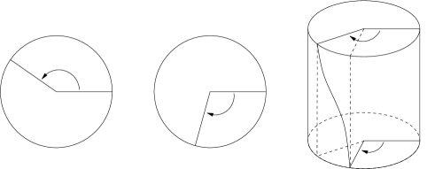
Figure 2. The local effect of $t$ on disk neighborhoods of $P$ and $Q$ in $F$, and the effect of $h$ on the neighborhood $N$ of $C$ in $G$. Only the boundaries of the disk neighborhoods are contained in $G$, where they form the boundary of $N$. The condition $a+b=ab\bmod n$ holds when the angle at $P$ is $2\pi a^{-1}/n$ and the angle at $Q$ is $2\pi(1-a^{-1})/n$.

$p$ [B] at 272 68 $q$ [B] at 225 92 $x_{0}$ [B] at 152 14 $x_{1}$ [B] at 180 95 $x_{2}$ [B] at 126 95 $x_{3}$ [B] at 72 95 $\alpha$ [B] at 312 102 $\beta$ [B] at 258 138 $\gamma_{1}$ [B] at 182 152

Figure 3. A quotient orbifold $\operatorname{{\mathcal{O}}}$, for the case $m=3$ and $g_{0}=2$.

Now, let $\operatorname{{\mathcal{O}}}$ be the quotient orbifold for the action of $C_{n}$ on $F$, and let $g_{0}$ be the genus of the underlying $2$-manifold $|\operatorname{{\mathcal{O}}}|$. Figure 3 shows $\operatorname{{\mathcal{O}}}$, with cone points $p$ and $q$ of order $n$ (the images of the points $P$ and $Q$ of $F$) and possibly other cone points $x_{1},\ldots\,$, $x_{m}$ of some orders $n_{1}\ldots\,$, $n_{m}$. The figure also shows some of the generators $\alpha$, $\beta$, and $\gamma_{1}$ of $\pi_{1}^{orb}(\operatorname{{\mathcal{O}}})$. Along with similar generators $\gamma_{i}$ going around the other $x_{i}$ and standard generators $a_{j}$ and $b_{j}$, $1\leq j\leq g_{0}$ in the “surface part” of $\operatorname{{\mathcal{O}}}$, we have a presentation

$$\pi_{1}^{orb}(\operatorname{{\mathcal{O}}})=\langle\alpha,\beta,\gamma_{1},\ldots,\gamma_{m},a_{1},b_{1},\ldots,a_{g_{0}},b_{g_{0}}\;|\;$$

$$\alpha^{n}=\beta^{n}=\gamma_{1}^{n_{1}}=\cdots=\gamma_{m}^{n_{m}}=1,\;\alpha\beta\gamma_{1}\cdots\gamma_{m}=\prod_{j=1}^{g_{0}}[a_{j},b_{j}]\;\rangle$$

$p$ [B] at 72 62 $\widetilde{x_{0}}$ [B] at 158 68 $\widetilde{\alpha}$ [B] at 150 90 $t(\widetilde{x_{0}})$ [B] at 47 148 $t^{a}(\widetilde{x_{0}})$ [B] at 155 110

Figure 4. The lift of $\alpha$ to $F$ starting at $\widetilde{x_{0}}$.

From orbifold covering space theory, the orbifold covering map $F\to\operatorname{{\mathcal{O}}}$ corresponds to an exact sequence

$$1\longrightarrow\pi_{1}(F)\longrightarrow\pi_{1}^{orb}(\operatorname{{\mathcal{O}}})\stackrel{{\scriptstyle\rho}}{{\longrightarrow}}C_{n}\longrightarrow 1\ .$$

Here, $C_{n}$ is the group of covering transformations, generated by $t$, and $\rho$ is obtained by lifting path representatives of elements of $\pi_{1}^{orb}(\operatorname{{\mathcal{O}}})$— these do not pass through the cone points so the lifts are uniquely determined. To find $\rho(\alpha)$, we note first that the loop $\alpha$ lifts as shown in Figure 4, so $\rho(\alpha)$ maps to $t^{a}$ where $t^{a}$ has rotation angle $2\pi/n$ about $P$. Since $t$ acts with rotation angle $2\pi k/n$, we have $ka=1\bmod n$ so $k=a^{-1}\bmod n$. Similarly at $Q$, the rotation angle of $t$ is $2\pi b^{-1}/n$. Since $h^{n}=t_{g+1}$, the left-hand twisting angle along $N$ in Figure 2 is $2\pi/n$. This requires $2\pi b^{-1}n-(-2\pi a^{-1}/n)=2\pi/n$, giving $b^{-1}+a^{-1}=1\bmod n$. Multiplying by $ab$ produces condition (iii) of a data set.

For $1\leq i\leq m$, the preimage of $x_{i}$ consists of $n/n_{i}$ points cyclically permuted by $t$. Each of the points has stabilizer generated by $t^{n/n_{i}}$. The rotation angle of $t^{n/n_{i}}$ must be the same at all points of the orbit, since its action at one point is conjugate by a power of $t$ to its action at each other point. So the rotation angle at each point is of the form $2\pi c_{i}^{\prime}/n_{i}$, where $\gcd(c_{i}^{\prime},n_{i})$, and as before, lifting $\gamma_{i}$ shows that $\rho(\gamma_{i})=(t^{n/n_{i}})^{c_{i}}$ where $c_{i}=(c_{i}^{\prime})^{-1}\bmod n_{i}$.

Finally, we have $\rho(\prod_{j=1}^{g_{0}}[a_{j},b_{j}])=1$, since $C_{n}$ is abelian, so

$$1=\rho(\alpha\beta\gamma_{1}\cdots\gamma_{m})=t^{a+b+(n/n_{1})c_{1}+\cdots+(n/n_{m})c_{m}}\ ,$$

giving condition (iv) of a data set.

The fact that the genus of the data set equals $g$ follows from the multiplicativity of the orbifold Euler characteristic for the orbifold covering $F\to\operatorname{{\mathcal{O}}}$:

$$(2-2g)/n=2-2g_{0}+2\Big{(}\frac{1}{n}-1\Big{)}+\sum_{i=1}^{m}\Big{(}\frac{1}{n_{i}}-1\Big{)}\ .$$

Thus $h$ leads to a data set of degree $n$ and genus $g$.

Suppose now that $h$ interchanges the sides of $C$. Its degree must be even, and we will write it as $2n$. The points $P$ and $Q$ are now interchanged by $t$, while $h^{2}$ is a root of $t_{g+1}$ of order $n$ that does not interchange the sides. In particular, $n$ must be odd. We assume for now that $n\geq 3$.

Let $D_{P}$ and $D_{Q}$ be the disks centered at $P$ and $Q$, for which $D_{P}\cup D_{Q}=\overline{F-F_{0}}$. The actions of $t^{2}$ at $P$ and $Q$ are conjugate, by $t$, so there exists an equivariant homeomorphism from $D_{Q}\cup D_{P}$ to $D^{2}\times\{-1,1\}$, where the latter has the action $t^{2}(x,-1)=(\exp(2\pi ik/n)\,x,-1)$ and $t^{2}(x,1)=(\exp(-2\pi ik/n)\,x,1)$ (the minus sign is not necessary, but is natural for our construction). We think of $P$ and $Q$ as corresponding to $\{0\}\times\{1\}$ and $\{0\}\times\{-1\}$ respectively.

Since $2\pi k/n$ is twice $2\pi k/(2n)$ and twice $2\pi(k+n)/(2n)$, we may further assume that the action of $t$ on $D^{2}\times\{-1,1\}$ in these coordinates is either $t(x,-1)=(\exp(-2\pi ik/(2n))\,\overline{x},1)$ and $t(x,1)=(\exp(2\pi ik/(2n))\,\overline{x},-1)$, or $t(x,-1)=(\exp(-2\pi i(k+n)/(2n))\,\overline{x},1)$ and $t(x,1)=(\exp(2\pi i(k+n)/(2n))\,\overline{x},-1)$.

Figure 5 illustrates the effect of $t$ on $\partial N$ for the first action, in which $t(x,1)=(\exp(2\pi ik/(2n))\,\overline{x},-1)$. The indicated angles are $2\pi k/(2n)$. If we extend $h_{0}$ to $N$ by sending $(x,t)$ to $(\overline{x},1-t)$ followed by a simple left-hand twist, as in Figure 5, then the twisting angle is $2\pi k/n$, and consequently $h^{2n}=t_{g+1}^{2k}$. Other extensions to $N$ will differ from this by full twists, giving $h^{2n}=t^{2k+2jn}$ for some integer $j$. In any case, $h^{2n}$ cannot equal $t_{g+1}$. For the second action, in which $t(x,1)=(\exp(2\pi i(k+n)/(2n))\,\overline{x},-1)$, the amount of twisting on $N$ is still $2\pi k/n$ plus some number of full twists, so again $h^{2n}=t^{2k+2jn}$.

$B$ [B] at 165 32 $A$ [B] at 165 177 $t(B)$ [B] at 78 129 $t(A)$ [B] at 77 79 $t^{2}(B)$ [B] at -17 55 $t^{2}(A)$ [B] at -17 155

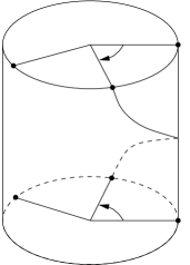
Figure 5. An extension of $t$ to $N$ in case $h$ interchanges the sides of $C$. The amount of left-hand twisting on $N$ is $2\pi k/n$, so $h^{2n}=t_{g+1}^{2k}$.

Finally, suppose that $n=1$. Then in the previous construction, $t^{2}$ is the identity on $D^{2}\times\{-1,1\}$, and $t$ is either $t(x,-1)=(\overline{x},1)$ and $t(x,1)=(\overline{x},-1)$, or $t(x,-1)=(-\,\overline{x},1)$ and $t(x,1)=(-\,\overline{x},-1)$. In either case, any extension of $h_{0}$ to $N$ has some number of full twists, so $h^{2}$ is some even power of $t_{C}$.

At this point, we have shown how every root of $t_{g+1}$ produces a data set. If the original roots are conjugate in $\operatorname{Mod}(G)$, then their restrictions to $F_{0}$ are conjugate and isotopic to conjugate homeomorphisms of order $n$, and their extensions to $F$ are conjugate by a homeomorphism preserving $\{P,Q\}$. Therefore their orbifold quotients $\operatorname{{\mathcal{O}}}$ and $\operatorname{{\mathcal{O}}}^{\prime}$ are homeomorphic by an orientation-preserving orbifold homeomorphism preserving taking the distinguished cone points $\{p,q\}$ to the distinguished cone points $\{p^{\prime},q^{\prime}\}$ of $\operatorname{{\mathcal{O}}}^{\prime}$, and compatible with the representations of the orbifold fundamental groups to $C_{n}$. It follows that our procedure produces equivalent data sets.

Given a data set, we can reverse the argument to produce the root $h$. We construct the corresponding orbifold $\operatorname{{\mathcal{O}}}$ and representation $\rho\colon\pi_{1}^{orb}(\operatorname{{\mathcal{O}}})\to C_{n}$. Any finite subgroup of $\pi_{1}^{orb}(\operatorname{{\mathcal{O}}})$ is conjugate to a subgroup of one of the cyclic subgroups generated by $\alpha$, $\beta$, or a $\gamma_{i}$, so condition (ii) ensures that the kernel of $\rho$ is torsionfree. Therefore the orbifold covering $F\to\operatorname{{\mathcal{O}}}$ corresponding to the kernel is a manifold, and calculation of its Euler characteristic shows that $F$ has genus $g$. Removing disks around the fixed points $P$ and $Q$ corresponding to the cone points $p$ and $q$ produces the surface $F_{0}$, and attaching an annulus $N$ produces the surface $G$ of genus $g+1$. Condition (iii) ensures that the rotation angles work correctly to allow an extension of $t|_{F_{0}}$ to an $h$ with $h^{n}$ a single Dehn twist.

It remains to show that the resulting root of $t_{g+1}$ is determined up to conjugacy. Our data sets encode the fixed-point data of the periodic transformation $t$, and it was proven by J. Nielsen [10] that this data determines $t$ up to conjugacy. We require in addition that the conjugating homeomophism preserve $\{P,Q\}$.

Suppose that $h$ and $h^{\prime}$ are roots obtained by applying our procedure to a data set $(n,g_{0},(a,b);(c_{1},n_{1}),\ldots,(c_{m},n_{m}))$. That is, we use the data set to define orbifolds $\operatorname{{\mathcal{O}}}$ and $\operatorname{{\mathcal{O}}}^{\prime}$ and homomorphisms $\rho\colon\pi_{1}^{orb}(\operatorname{{\mathcal{O}}})\to C_{n}$ and $\rho^{\prime}\colon\pi_{1}^{orb}(\operatorname{{\mathcal{O}}}^{\prime})\to C_{n}$, then take the corresponding covers $F$ and $F^{\prime}$ and so on. Each of $\operatorname{{\mathcal{O}}}$ and $\operatorname{{\mathcal{O}}}^{\prime}$ has genus $g_{0}$ and $m+2$ cone points of corresponding orders, including the two distinguished order-$n$ cone points, which give elements $\alpha$ and $\beta$ and $\pi_{1}^{orb}(\operatorname{{\mathcal{O}}})$ and $\alpha^{\prime}$ and $\beta^{\prime}$ and $\pi_{1}^{orb}(\operatorname{{\mathcal{O}}}^{\prime})$. We have $\rho(\alpha)=\rho^{\prime}(\alpha^{\prime})=t^{a}$, where the rotation angles of $t$ and $t^{\prime}$ at $P$ are $2\pi a^{-1}/n$, and similarly for the other generators coming from cone points.

We claim that the generators $a_{i}$ and $b_{i}$ of $\pi_{1}^{orb}(\operatorname{{\mathcal{O}}})$ may be selected so that $\rho(a_{i})=\rho(b_{i})=1$ for all $i$. Suppose this is not initially the case. There is an orbifold homeomorphism of $\operatorname{{\mathcal{O}}}$ whose effect on the abelianization of $\pi_{1}^{orb}(\operatorname{{\mathcal{O}}})$ is to send $\overline{a_{1}}$ to $\overline{a_{1}}\overline{\alpha}$ and to fix the other generators; it is the end map of an isotopy that slides the cone point $p$ around a loop that represents $\overline{b_{1}}$. Since $\rho(\alpha)$ is a generator of $C_{n}$, we may repeat this homeomorphism some number of times until for the new $a_{1}$, $\rho(\overline{a_{1}})=1$. Repeating this process on the other $a_{i}$ and $b_{i}$, we obtain a new set of generators that verify the claim.

Performing a similar process, we may assume that $\rho^{\prime}(a_{i}^{\prime})=\rho^{\prime}(b_{i}^{\prime})=1$ for all $i$. Now, we take an orientation-preserving orbifold homeomorphism $k\colon\operatorname{{\mathcal{O}}}\to\operatorname{{\mathcal{O}}}^{\prime}$ such that $k_{\#}(\alpha)=\alpha^{\prime}$ and so on. It satisfies $\rho^{\prime}\circ k_{\#}=\rho$, so $k$ lifts to a homeomorphism $K\colon F\to F^{\prime}$ such that $KtK^{-1}=t^{\prime}$. If we select $k$ with a bit of care, $K$ carries $F_{0}$ to $F_{0}^{\prime}$, and we can extend $K|_{F_{0}}$ to a homeomorphism of $G$ conjugating $h$ to $h^{\prime}$. ∎

Theorem 1.1 tells us that $t_{g+1}$ always has a cube root when $g\geq 1$, corresponding to the data sets $(3,0,(2,2);(c_{1},3),\ldots,(c_{g},3))$ with the $c_{i}$ selected to achieve condition (iv). Also, if $t_{g+1}$ has a root of degree $n$, then replacing $g_{0}$ by $g_{0}+1$ in a corresponding data set produces a root of degree $n$ for $t_{g+n+1}$.

Of more interest is the following:

Corollary 1.2.

Suppose that $t_{g+1}$ has a root of degree $n$. Then

1. $n$ is odd.

2. $n\leq 2g+1$.

Proof.

Part (a) is simply the fact that data sets must have odd degree. For (b), suppose for contradiction that $n>2g+1$. From the formula for $g$, we have $1>(2g+1)/n=1/n+2g_{0}+\sum_{i=1}^{m}(1-1/n_{i})$ so $g_{0}=0$, $m=1$, and $n_{1}<n$. Putting $d=n/n_{1}$, condition (iv) gives $a+b=0\bmod d$, contradicting condition (iii) since $1<d$ and $d$ divides $n$. ∎

It may be of interest to note that the maximum degree of a root is half of the maximum order $4g+2$ of a periodic homeomorphism of $F$, found by A. Wiman [12] and W. Harvey [4].

2. The Margalit-Schleimer roots

Here we will describe the examples of Margalit and Schleimer from our viewpoint. They construct the surface $F$ by identifying opposite faces of a $(4g+2)$-gon. It center point is $X_{1}$, and the two points that come from identifying vertices are $P$ and $Q$. Pictures centered at $X_{1}$, $P$, and $Q$ are shown in Figure 6 for the case of $g=2$; in general $e_{4}$ becomes $e_{2g}$, and so on. Let $f$ be the homeomorphism of $F$ obtained by rotating through a (counterclockwise) angle of $2\pi/(2g+1)$ at $P$ and $Q$. It carries $e_{0}$ to $e_{1}$, so it rotates through an angle of $2\pi g/(2g+1)$ at $X_{1}$. Let $t$ be $f^{-g}$, which rotates through $2\pi(g+1)/(2g+1)$ at $P$ and $Q$ and through $-2\pi g^{2}/(2g+1)$ at $X_{1}$. Modulo $2g+1$, $-g^{2}$ is $g/2$ if $g$ is even and $-(g+1)/2$ if $g$ is odd, so $t$ is approximately a quarter turn at $X_{1}$, counterclockwise if $g$ is even and clockwise if not. The examples are then obtained by the construction in Theorem 1.1.

$X_{1}$ [B] at 240 120 $P$ [B] at 750 120 $Q$ [B] at 1280 120 $Q$ [B] at 140 415 $P$ [B] at 280 415 $X_{1}$ [B] at 660 415 $Q$ [B] at 800 415 $X_{1}$ [B] at 1180 415 $P$ [B] at 1320 415 $P$ [B] at 15 315 $Q$ [B] at 410 315 $Q$ [B] at 535 315 $X_{1}$ [B] at 940 315 $P$ [B] at 1065 315 $X_{1}$ [B] at 1465 315 $Q$ [B] at -28 190 $P$ [B] at 440 190 $X_{1}$ [B] at 495 190 $Q$ [B] at 965 190 $X_{1}$ [B] at 1015 190 $P$ [B] at 1490 190 $P$ [B] at 10 60 $Q$ [B] at 405 60 $Q$ [B] at 533 60 $X_{1}$ [B] at 935 60 $P$ [B] at 1060 60 $X_{1}$ [B] at 1460 60 $Q$ [B] at 140 -40 $P$ [B] at 280 -40 $X_{1}$ [B] at 660 -40 $Q$ [B] at 800 -40 $X_{1}$ [B] at 1180 -40 $P$ [B] at 1320 -40 $e_{0}$ [B] at 215 415 $e_{4}$ [B] at 65 370 $e_{1}$ [B] at 350 370 $e_{3}$ [B] at -10 260 $e_{2}$ [B] at 430 260 $e_{2}$ [B] at -10 140 $e_{3}$ [B] at 430 140 $e_{1}$ [B] at 65 20 $e_{4}$ [B] at 350 20 $e_{0}$ [B] at 215 -30 $e_{0}$ [B] at 880 215 $e_{0}$ [B] at 1390 215 $e_{1}$ [B] at 752 340 $e_{1}$ [B] at 1277 340 $e_{2}$ [B] at 600 260 $e_{2}$ [B] at 1115 260 $e_{3}$ [B] at 628 85 $e_{3}$ [B] at 1150 85 $e_{4}$ [B] at 812 55 $e_{4}$ [B] at 1335 55

Figure 6. The configurations of the edges $e_{i}$ around $P$ and $Q$, as seen from $X_{1}$, $P$, and $Q$ in the Margalit-Schleimer example for $g=2$.

The inverse of $g+1\bmod 2g+1$ is $2$, so $a=b=2$, while the inverse of $-g^{2}$ is $c_{1}=-4$. So the data set resulting from the Margalit-Schleimer construction is $(2g+1,0,(2,2);(-4,2g+1))$.

We call a root of $t_{g+1}$ a Margalit-Schleimer root if it has degree $2g+1$. Using Theorem 1.1, is is easy to find all the Margalit-Schleimer roots. We need only find the $x\bmod n$ such that $x$ and $1-x$ are both relatively prime to $n$, then put $a=x^{-1}$ and $b=(1-x)^{-1}\bmod n$, and $c_{1}=-a-b\bmod n$. A GAP function to list such roots is provided in the software at [9]. For example, we find that $t_{11}$ has three Margalit-Schleimer roots, $(21,0,(2,2);(17,21))$, $(21,0,(5,17);(20,21))$, and $(21,0,(11,20);(11,21))$, and $t_{1,001}$ has $284$.

3. Genus sets

The genus set of $n$, $g(n)$, is the set of $g$ such that $t_{g+1}$ has a root of degree $n$. Corollary 1.2 tells us that $g(n)$ is empty for even $n$. For odd $n$, we can gain considerable information about the genus set. For the rest of this section, $n$ will be assumed odd, and $n_{0}$ will denote $(n-1)/2$.

A data set with all $n_{i}=n$ is called a primary data set, and the corresponding root of $t_{g+1}$ is called a primary root. Primary data sets exist for all $m\geq 1$, since we may take $a=b=2$, and the $c_{i}$ selected from ${-4,-2,1,-1}$ so that $a+b+\sum c_{i}=0\bmod n$.

We now examine the genera of primary data sets. A quick example will make it much easier to follow the notation. For $n=9$, so that $n_{0}=4$, we position the genera according to their values $\bmod\ n_{0}$:

(0) (1) (2) (3)

4 (5) (6) (7)

8 (9) (10) (11)

12 13 (14) (15)

16 17 (18) (19)

20 21 22 (23)

24 25 26 (27)

28 29 30 31

The genus of a primary data set $(n,g_{0},(a,b);(c_{1},n),\ldots,(c_{m},n))$ is $ng_{0}+mn_{0}$. For $g_{0}=0$, we obtain the values $mn_{0}$ for $m\geq 1$, which for $n=9$ are the values in the first column other than $0$. For $g_{0}=1$, $n+mn_{0}$ is always $1\bmod n_{0}$, and we obtain all values greater than $n$. Similarly, $g_{0}=2$ gives the values in the third column greater than $2n$, and $g_{0}=3$ gives those in the last column beyond $3n$. Higher values of $g_{0}$ give no new values for $g$. So the primary data sets for $n=9$ give all values of $g$ except the $16$ values indicated in the table.

In general, the genera obtained from data sets of degree $n$ having $0\leq g_{0}<n_{0}$ are $g_{0}\bmod n_{0}$, and are exactly those with $g>g_{0}n$. No new genera are obtained when $g_{0}\geq n_{0}$. So the genera not obtained are those in the “triangular” set $T(n)$ defined by

$$T(n)=\cup_{0\leq g_{0}<n_{0}}T_{g_{0}}(n),\text{\ where}$$

$$T_{g_{0}}(n)=\{g_{0}+mn_{0}\;|\;0\leq m\leq 2g_{0}\}\ .$$

Since $T_{g_{0}}(n)$ has $2g_{0}+1$ elements, $T(n)$ has $n_{0}^{2}$ elements. The maximum element in $T(n)$ is the maximum element in $T_{n_{0}-1}(n)$, which is $(n_{0}-1)n=n(n-3)/2$.

Since the primary data sets produce roots for every genus other than those in $T(n)$, we have

Corollary 3.1.

For $n$ odd, $g(n)$ contains all $g\geq 0$ that are not in $T(n)$. Consequently, $t_{g+1}$ has a root of degree $n$ whenever $g+1>(n-2)(n-1)/2$.

When $n$ is prime, all data sets are primary. So we have

Corollary 3.2.

For $n$ prime, $g(n)$ equals the set of $g$ not in $T(n)$. In particular, $t_{(n-2)(n-1)/2}$ does not have a root of degree $n$.

For example, $t_{g+1}$ has a cube root for all $g+1\geq 2$, and a fifth root exactly when $g+1$ is not $1$, $2$, $4$, or $6$. For $n$ that are not prime, determination of $g(n)$ is more complicated, as elements in $T(n)$ often arise from non-primary data sets. For example, $7\notin T(9)$, but a ninth root for $t_{8}$ arises from the data set $(9,0,(2,2);(2,9),(1,3))$, for which condition (iv) is satisfied since $a+b+c_{1}+(9/3)c_{2}=0\bmod 9$.

We note that $T_{n}$ contains about half of the values with $g\leq n(n-3)/2$. Therefore in Figure 1, the pairs $(g,n)$ corresponding to primary roots would be about half of the pairs with $n$ odd in the region above $g=(n-1)(n-2)/2$.

4. The root set and $(d,e)$-roots

The root set $R(g)$ is the set of $n$ such that $t_{g+1}$ has a root of degree $n$ (although degree set would be a more accurate name). Corollary 3.2 allows us to effectively compute the primes in $R(g)$. From Corollary 3.1, $R(g)$ contains $n$ whenever $(n-2)(n-1)/2\leq g$. In Theorem 4.2, we will determine all $n$ in $R(g)$ that satisfy $n\geq g$. First, we must introduce $(d,e)$-roots.

Let $d$ and $e$ be odd integers with $d,e\geq 3$. A root corresponding to a data set having $g_{0}=0$, $m=2$, $n_{1}=d$ and $n_{2}=e$ is called a $(d,e)$-root. The next lemma requires an elementary number-theoretic fact for which we are unable to find a reference. To avoid interruption of the argument here, we will prove it later as Lemma 7.1.

Lemma 4.1.

For any odd integers $d,e\geq 3$, there exist $(d,e)$-roots. Such roots satisfy the following:

1. $n=\dfrac{de}{\gcd(d,e)}$, i. e. $n=\operatorname{lcm}(d,e)$.

2. $g=n-\dfrac{d+e}{2\gcd(d,e)}=n\Big{(}1-\dfrac{1}{2d}-\dfrac{1}{2e}\Big{)}$.

3. $g+1\leq n<6(g+2)/5$.

4. $n=g+1$ exactly when $d=e=n$.

For example, a $(3,5)$-root has $(g,n)=(11,15)$ (so Lemma 4.1(c) is best possible, in general), and for $n=105$ there are $(3,35)$-roots when $g=86$ and $(15,7)$-roots when $g=94$. For even $g$, there is always a $(g+1,g+1)$-root given by $(g+1,(2,2);(-2,g+1),(-2,g+1))$.

Proof of Lemma 4.1.

Put $d_{0}=\gcd(d,e)$ and $n=de/d_{0}$, so $\gcd(n/d,n/e)=1$. Let $n_{1}=d$, $n_{2}=e$, and $a=b=2$. Condition (iv) becomes $4+c_{1}(n/d)+c_{2}(n/e)=0$. Since $\gcd(n/d,n/e)=1$, we can write $\ell_{1}(n/d)+\ell_{2}(n/e)=1$, and by Lemma 7.1 we may assume that $\gcd(\ell_{1},d)=\gcd(\ell_{2},e)=1$. Taking $c_{1}=-4\ell_{1}$ and $c_{2}=-4\ell_{2}$ satisfies condition (iv). The genus works out to be the expressions in (b), which imply the first inequality in (c). For the second, we have

$$n=g+\frac{d+e}{2d_{0}}\leq g+\frac{3+\frac{de}{3}}{2d_{0}}=g+\frac{3}{2d_{0}}+\frac{1}{6}\frac{de}{d_{0}}<g+2+\frac{n}{6}\ .$$

Part (d) follows because (b) gives $n=g+1$ when $d=e=n$, and when $d\neq e$, $\dfrac{d+e}{2d_{0}}>1$ so $g+1<n$. ∎

For a given $n$ one can easily compute the $g$ for which $n$ is a $(d,e)$-root of $g$, if we have a prime factorization of $n$. For in (b) of Lemma 4.1, $n/d$ and $n/e$ are relatively prime divisors of $n$. For each pair $(d_{1},d_{2})$ of relatively prime divisors, we write $n=d_{0}d_{1}d_{2}$ and put $d=d_{0}d_{1}$ and $e=d_{0}d_{2}$ giving $n$ as a $(d,e)$-root for $g=n-(d_{1}+d_{2})/2$ by Lemma 4.1(b). This gives an algorithm for computing the $(d,e)$-roots of $g$, again assuming that we can factor, just by checking which of the $n$ in the range allowed by Lemma 4.1(c) have $g$ among its corresponding genera. We have implemented these algorithms as a GAP script [3] available at [9]. Some sample calculations include the genera having a $(d,e)$-root of degree $n$:

gap$>$ DERootGenera( 54573 );
[ 45476, 45477, 54571, 54572 ]

and all $(d,e)$-roots for a given genus:

gap$>$ DERoots( 54572 );
[ 54573, 54575, 54587, 54769, 65487 ]
gap$>$ DERoots( 54573 );
[ ]

The main result of this section describes all roots of large degree:

Theorem 4.2.

Suppose $t_{g+1}$ has a root of degree $n\geq g$. Then the root is either a Margalit-Schleimer root, a $(d,e)$-root, or the cube root of $t_{4}$.

Proof.

Since $n\geq g$, we have

$$1\geq\frac{g}{n}=g_{0}+\frac{1}{2}\sum_{i=1}^{m}\Big{(}1-\frac{1}{n_{i}}\Big{)}\geq 2g_{0}+\frac{m}{3}\ .$$

Therefore $g_{0}=0$ and $m\leq 3$.

Suppose first that $m=1$. We cannot have $n_{1}<n$, for putting $d=n/n_{1}$, condition (iv) would say that $a+b+dc_{1}=0\bmod n$, which is impossible since $a+b$ is relatively prime to $n$ and hence to $d$. So $n_{1}=g$, and $h$ is a Margalit-Schleimer root.

If $m=2$, then $h$ is a $(d,e)$-root.

Suppose that $m=3$. From our expression for $\frac{g}{n}$, we find that $1\leq\frac{1}{n_{1}}+\frac{1}{n_{2}}+\frac{1}{n_{3}}$. Since all $n_{i}$ are odd this can only be satisfied when $n_{1}=n_{2}=n_{3}=3$. Condition (iv) says that $a+b=0\bmod n/3$, a contradiction unless $n=3$. That is, $h$ is a cube root with $g=3$. In fact, this $h$ is unique, since the only data set of degree $3$ and genus $3$ is $(3,0,(2,2);(1,3),(2,3),(2,3))$. ∎

In view of Lemma 4.1(c), Theorem 4.2 has the amusing consequence that the only $t_{g+1}$ which has a root of degree $g$ is $t_{4}$.

5. There are no orientation-reversing roots

In this section, we will prove that $t_{g+1}$ has no orientation-reversing roots, and that roots of $t_{g+1}$ cannot be conjugate by orientation-reversing homeomorphisms. Consequently, Theorem 1.1 classifies all roots of $t_{g+1}$ in the homeomorphism group, up to conjugacy.

Proposition 5.1.

Let $h$ be an orientation-reversing homeomorphism of $G$ with $h^{n}$ isotopic to $t_{g+1}^{\ell}$ for some $n>0$. Then $\ell=0$.

Proof.

As in the proof of Theorem 1.1, we write $t_{g+1}=t_{C}$ and change $h$ by isotopy so that $h$ restricts to a homeomorphism $h_{0}$ of finite order on $\overline{G-N}$ for some annulus neighborhood $N$ of $C$. On $N$, $h$ is orientation-reversing and has finite order on $\partial N$.

Suppose first that $h$ preserves the components of $\partial N$. Then $h$ reverses orientation on each component, so is a reflection of period $2$. It follows that $h_{0}$ has order $2$, and for some coordinates on $N$ as $S^{1}\times I$, $h$ is isotopic to a homeomorphism of the form $(z,t)\mapsto(\overline{z},t)$. Therefore $h^{2}$ is isotopic to the identity on $G$, so $\ell=0$.

Suppose now that $h$ interchanges the components of $\partial N$. Since $h$ is orientation-reversing and has finite order on $\partial N$, there are coordinates on $\partial N$ as $S^{1}\times\{0,1\}$ so that $h(z,t)=(e^{2\pi k/n}z,1-t)$. Let $e$ be the homeomorphism of $N$ defined by $(z,t)\mapsto(e^{2\pi k/n}z,1-t)$. Then $h|_{N}$ is isotopic relative to $\partial N$ to $t_{C}^{r}e$ for some power $r$. Since $et_{C}$ is isotopic to $t_{C}^{-1}e$ relative to $\partial N$, and $n$ must be even, $h^{n}$ is isotopic to the identity, that is, $\ell=0$. ∎

We note also that no two roots of $t_{C}$ can be conjugate by an orientation-reversing homeomorphism. For if $h_{1}$ and $h_{2}$ are roots and $gh_{1}g^{-1}=h_{2}$ with $g$ orientation-reversing, then $gt_{C}g^{-1}=t_{C}$. But conjugation of a left-handed Dehn twist by an orientation-reversing homeomorphism produces a right-handed Dehn twist.

6. Roots of $t^{\ell}$

Theorem 1.1 gives some information about the roots of powers of $t_{g+1}$, that is, the fractional powers of $t_{g+1}$. A tuple like a data set except that condition (iii) is replaced by the condition that $a+b=\ell ab\bmod n$ produces a root of $t_{g+1}^{\ell}$ of degree $n$. The only difference in the construction is that the rotation angles at $P$ and $Q$ are of the form $2\pi k/n$ and $2\pi(\ell-k)/n$, and the twisting on the annulus $N$ is through an angle $2\pi\ell/n$ rather than $2\pi/n$. Thus the data set $(4,0,(1,1);(1,2))$ for which $a+b=2ab\bmod 4$ yields a root of $t_{2}^{2}$ of degree $4$. Of course we know from Corollary 1.2 that $t_{2}$ does not have a square root. The data set $(3,0,(1,1);(2,3),(2,3))$ gives a cube root of $t_{3}^{2}$.

There are some complications, however. If $\ell$ and $n$ are not relatively prime, then a root of degree $n$ of $t_{g+1}^{\ell}$ might be a power of a root of a smaller power of $t_{g+1}$ of lower degree, and then the action on $F$ in the proof of Theorem 1.1 will not be effective. More interesting is the fact that roots of $t_{g+1}^{\ell}$ may exchange the sides of $C$, requiring a different kind of quotient orbifold to be analyzed.

7. An elementary lemma

In Section 4 we needed an elementary number-theoretic fact, Lemma 7.1. We are grateful to Ralf Schmidt for providing us with a much better proof than our original one.

Lemma 7.1.

Let $d_{1}$, $d_{2}$ be relatively prime positive integers, and let $Q$ be a finite set of primes. If $2\in Q$, assume that $d_{1}$ and $d_{2}$ are not both odd. Then there exist integers $c_{1}$ and $c_{2}$ so that $c_{1}d_{1}+c_{2}d_{2}=1$ and neither $c_{1}$ nor $c_{2}$ is divisible by any prime in $Q$.

Proof.

Choose $A$ and $B$ with $Ad_{2}+Bd_{1}=1$, so that $(A-kd_{1})d_{2}+(B+kd_{2})d_{1}=1$ for all integers $k$. We seek a $k$ so that $A-kd_{1}$ and $B+kd_{2}$ are nonzero $\bmod q_{i}$ for each $q_{i}\in Q$.

For each odd $q_{i}\in Q$, if any $A-kd_{1}=0\bmod q_{i}$, then $\gcd(q_{i},d_{1})=1$. So there is a unique $k_{i}\bmod q_{i}$ such that $A-kd_{1}=0\bmod q_{i}$ exactly when $k=k_{i}\bmod q_{i}$. Similarly, if any $B+kd_{2}=0\bmod q_{i}$, then such $k$ are those with $k=\ell_{i}\bmod q_{i}$ for a unique $\ell_{i}\bmod q_{i}$. Since $q_{i}\geq 3$, there are choices of $m_{i}$ so that if $k=m_{i}\bmod q_{i}$, then neither $A-kd_{1}=0\bmod q_{i}$ nor $B+kd_{2}=0\bmod q_{i}$. If $q_{i}=2$, then we may assume that $d_{2}$ is even and $d_{1}$ and hence $B$ are odd, and we take $m_{i}$ equal to $0$ or $1$ according as $A$ is odd or even. The $k$ we are seeking include all those satisfying $k=m_{i}\bmod q_{i}$ for all $i$, and such $k$ exist by the Chinese Remainder Theorem. ∎

References

- [1] W. Fenchel, Estensioni di gruppi discontinui e transformazioni periodiche delle superficie, Atti Accad. Naz Lincei. Rend. Cl. Sci. Fis. Mat. Nat. (8) 5 (1948), 326–329.
- [2] W. Fenchel, Remarks on finite groups of mapping classes, Mat. Tidsskr. B 1950 (1950), 90–95.
- [3] GAP: Groups, Algorithms, and Programming, available at the St. Andrews GAP website http://turnbull.mcs.st-and.ac.uk/gap/
- [4] W. J. Harvey, Cyclic groups of automorphisms of a compact Riemann surface, Quart. J. Math. Oxford Ser. (2) 17 (1966), 86–97.
- [5] S. Kerckhoff, The Nielsen realization problem, Bull. Amer. Math. Soc. (N.S.) 2 (1980), 452–454.
- [6] S. Kerckhoff, The Nielsen realization problem, Ann. of Math. (2) 117 (1983), 235–265.
- [7] D. Margalit and S. Schleimer, Dehn twists have roots, Geom. Topol. 13 (2009) 1495–1497.
- [8] J. Nielsen, Abbildungklassen Endliche Ordung, Acta Math. 75 (1943), 23-115.
-
[9]
D. McCullough, Software for “Roots of Dehn twists”,
available at
http://www.math.ou.edu/dmccullough/research/software.html - [10] J. Nielsen, Die Struktur periodischer Transformationen von Flächen, Danske Vid. Selsk. Mat.-Fys. Medd. 1 (1937) 1-77.
-
[11]
W. Thurston, The Geometry and Topology of
Three-Manifolds, available at
http://msri.org/publications/books/gt3m - [12] A. Wiman, Über die hyperelliptischen Curven und diejenigen vom Geschlechte , welche eindeutigen Transformationen in sich zulassen, Bihang Kongl. Svenska Vetenskaps-Akademiens Handlinger, Stockholm, 1895-1896.
- [13] H. Zieschang, Finite groups of mapping classes of surfaces, Lecture Notes in Mathematics, 875. Springer-Verlag, Berlin, 1981.