Frustrated Bose condensates in optical lattices

Abstract

We study the Bose-condensed ground states of bosons in a two-dimensional optical lattice in the presence of frustration due to an effective vector potential, for example, due to lattice rotation. We use a mapping to a large-$S$ frustrated magnet to study quantum fluctuations in the condensed state. Quantum effects are introduced by considering a $1/S$ expansion around the classical ground state. The large-$S$ regime should be relevant to systems with many particles per site. As the system approaches the Mott insulating state, the hole density becomes small. Our large-$S$ results show that, even when the system is very dilute, the holes remain a (partially) condensed system. Moreover, the superfluid density is comparable to the condensate density. In other words, the large-$S$ regime does not display an instability to noncondensed phases. However, for cases with fewer than 1/3 flux quantum per lattice plaquette, we find that the fractional condensate depletion increases as the system approaches the Mott phase, giving rise to the possibility of a noncondensed state before the Mott phase is reached for systems with smaller $S$.

I Introduction

Bosonic atoms in optical lattices can display superfluid and Mott insulating phases. If the system is rotated, then, in the corotating frame, this is equivalent to introducing an effective magnetic field proportional to the rotation frequency CooperReview ; Bhat . This is not the only means to introduce a vector potential to a system of neutral atoms. This can also be achievedFurtado ; Pachos ; Pachos2 ; Kay through the interaction of atomic electric and magnetic moments with an external electromagnetic field (Aharonov-Casher and differential Aharonov-Bohm effects). For atoms trapped in an optical lattice in two distinct internal states, a scheme Jaksch using two additional Raman lasers combined with the lattice acceleration or inhomogeneous static electric field has also been proposed.

Bosonic atoms in an optical lattice can be modeled by a Bose-Hubbard model. A vector potential introduces an Aharonov-Bohm phase for the boson hopping from site to site. The wave function is “frustrated” if the phase twists around each plaquette add up to $2\pi\alpha$ for some non-integer $\alpha$. For a Bose condensate at a low effective magnetic field, this introduces vortices into the condensate. The presence of the optical lattice Sorensen ; Bhat interferes with the formation of an Abrikosov vortex lattice Williams ; CooperReview and quantum fluctuations may be enhanced. Further, if the number of vortices becomes comparable to the number of bosons, the system may enter into a fractional quantum Hall state CooperReview ; Wilkin ; Cooper ; Rezayi ; Sorensen ; Bhat . However, this requires a very high rotation frequency or a low atomic density which is hard to achieve experimentally.

In this work, we will focus on the experimentally accessible regime where a condensate still exists to examine whether there are any precursors to such states in a frustrated Bose condensate. We study a two-dimensional (2D) Bose-Hubbard model on a square lattice for a range of incommensurate filling. In the regime of strong on-site interaction, the model is analogous to a quantum easy-plane ferromagnet and the frustration encourages spin twists, i.e., the formation of vortices in the ground state. We find the classical ground states using Monte Carlo methods and then we study the quantum fluctuations around the classical state. In other words, we work under the assumption that quantum effects do not change qualitatively the nature of the ordering obtained for the classical ground states. Mathematically, this means that we will work in a large-$S$ generalization of the spin model and perform an expansion in $1/S$ to obtain the quantum effects. Although our original model corresponds to small $S$, the large-$S$ approach can be justified if the perturbative series in $1/S$ convergesCanali ; Igarashi ; Chubukov ; Kollar ; Bernardet . In those cases, a spin wave calculation may give accurate results.

We will study how quantum fluctuations affect the order parameter, off-diagonal long-range order (ODLRO) and the superfluid fraction for different degrees of frustration for the whole range of incommensurate filling. In the spin analog, the incommensurate filling corresponds to a range of Zeeman field $h$ up to some frustration-dependent critical field $h_{c}(\alpha)$. Our calculations were made for $\alpha=0,1/4,1/3$, and 1/2.

Our results show that the degree of Bose condensation decreases as $h$ increases toward $h_{c}$. However, it does not vanish at the limit of $h=h_{c}(\alpha)$. This applies to several quantities that we have calculated: the reduction in the order parameter, the reduction in the largest eigenvalue of the density matrix, and the sum of the non-macroscopic eigenvalues of the density matrix. We also find similar conclusions for the superfluid fraction — frustration reduces the superfluid fraction in the comparison with the unfrustrated case but there is no vanishing of the superfluid fraction at any $h\leq h_{c}$.

The paper is organized as follows. We will outline the model and the mapping to the quantum spin model in Sec. II. We describe the classical ground states ($S\rightarrow\infty$) of the spin analog in Sec. III. We introduce the excitations above the ground state in a $1/S$ expansion in Sec. IV. In Secs. V and VI, we calculate the degree of condensation and superfluidity in the system. We make conclusions about our study in the final section.

II Model Hamiltonian

For atoms trapped in a two-dimensional optical lattice, we can focus on a single-band lattice model if the tunneling $t$ between wells within the lattice is weak compared to the level spacings in each well. If the tunneling is also weak compared to the repulsive energy $U$ for two atoms in one well, then strongly correlated ground states, such as the Mott insulator, appear as well as a superfluid state.

Many different methods have been proposed to introduce frustration in the atomic motion. This can be done through rotating the systemCooperReview or through the interaction of the atoms with an external electromagnetic field Furtado ; Pachos ; Pachos2 ; Kay . If there is only one species of bosonic atoms, then the system is described by a Bose-Hubbard model on a square lattice with a complex hopping matrix element: $H_{\rm Hubbard}=H^{(0)}+V$ with

$$H^{(0)} = \frac{U}{2}\sum_{i}\hat{a}^{\dagger}_{i}\hat{a}_{i}(\hat{a}^{\dagger}_{i}\hat{a}_{i}-1)-\sum_{i}\mu\hat{a}^{\dagger}_{i}\hat{a}_{i},$$

$$T = -t\sum_{\langle ij\rangle}\left(e^{i\phi_{ij}}\hat{a}_{j}^{\dagger}\hat{a}_{i}+\mbox{H.c.}\right),$$ (1)

where $\mu$ is the chemical potential and $\langle ij\rangle$ denotes nearest-neighbor sites $i$ and $j$. The complex tunneling couplings appear in the Hubbard Hamiltonian due to the presence of the effective vector potential $\vec{A}$. When an atom moves from a lattice site at $\vec{R}_{i}$ to a neighboring site at $\vec{R}_{j}$, it will gain an Aharonov-Bohm phase

$$\phi_{ij}=\int_{\vec{R}_{i}}^{\vec{R}_{j}}\vec{A}\cdot d\vec{r},$$ (2)

For neutral atoms with electric moments $\vec{d}_{e}$ and a magnetic moments $\vec{d}_{m}$ in an external electromagnetic field $(\vec{E},\vec{B})$, $\vec{A}=(\vec{d}_{m}\times\vec{E}+\vec{d}_{e}\times\vec{B})/\hbar c$ Furtado ; Pachos ; Pachos2 ; Kay . For a rotating lattice, $\vec{A}=m\vec{\Omega}\times\vec{r}/\hbar$, where $\vec{\Omega}$ is the rotation frequency and $m$ is the mass of the atom. In this work, we study the case of the uniform effective magnetic field $\vec{B}=\vec{\nabla}\times\vec{A}=B\hat{z}$. Results will depend on the frustration parameter $\alpha$, defined as the flux per plaquette in units of $2\pi$,

$$\alpha=\frac{1}{2\pi}\int\vec{B}\cdot d\vec{S}_{\rm plaq}=\frac{1}{2\pi}\sum_{\rm plaq}\phi_{ij}$$ (3)

where the integration is over the surface of a lattice plaquette and the sum is performed anticlockwise over the edges of the square plaquette. This parameter is only meaningful between 0 and 1 because a flux of $2\pi$ through a plaquette has no effect on the system. Frustration is maximal at $\alpha=1/2$.

In this paper, we will use a magnetic analogy as the framework to study the Bose-Hubbard problem. This is most easily motivated in the limit of $U/t\to\infty$, even though we will not be working directly in this limit. In such a limit, the site occupation can be restricted to zero and one boson. Then, the Hilbert space of possible states can be mapped onto a spin-half XY model. The two $S_{z}$ states of the pseudospin correspond to whether a lattice contains a boson or not.

The spin raising and lowering operators correspond to the creation and annihilation of hard-core bosons, respectively. This mapping is possible because hard-core bosons have the same commutation relations as $S=1/2$ operators: operators on different sites commute but operators on the same site anticommute. The motion of the atoms translates to pseudospin exchange. The effective Hamiltonian is

$$H_{eff}=-\frac{J}{2}\sum_{\langle ij\rangle}\left(e^{i\phi_{ij}}\hat{S}_{i}^{+}\hat{S}_{j}^{-}+\mbox{H.c.}\right)-h\sum_{j}\hat{S}_{j}^{z}$$ (4)

where $J=2t$, $\hat{S}_{i}^{\pm}=\hat{S}^{x}_{i}\pm\hat{S}^{y}_{i}$ are the spin-$1/2$ operators, and $h=\mu$ represents an effective Zeeman field. Note that this is a ferromagnet in the absence of frustration ($\phi_{ij}=0$).

It is not simple to attack the infinite-$U$ limit of the problem of hard-core boson directly. Instead, we will relax the hard-core condition and allow for more than one boson on each site. We will allow $2S$ atoms on each site so that each site has $2S+1$ possible states. This corresponds to a spin-$S$ model with the Hamiltonian given in Eq. (4). The relationship between the original bosons, $\hat{a}$, and this spin-$S$ model is established via the Holstein-Primakoff representation:

$$\hat{S}_{i}^{+}=\hat{c}^{\dagger}_{i}(2S-\hat{c}^{\dagger}_{i}\hat{c}_{i})^{1/2},\qquad\hat{S}_{i}^{z}=\hat{c}^{\dagger}_{i}\hat{c}_{i}-S.$$ (5)

where $\hat{c}_{i}$ are operators with bosonic commutations and are essentially the original bosons $\hat{a}_{i}$ of the Bose-Hubbard model. The limit of $S\rightarrow\infty$ corresponds to the classical limit of the model. More specifically, we need $S\rightarrow\infty$ while $JS$ and $h$ remain constant so that exchange and Zeeman energies remain comparable.

Mathematically, the large-$S$ limit provides a systematic way to control the quantum fluctuations in this problem. Quantum fluctuations can be introduced (see later) in a $1/S$ expansion under the assumption that those effects do not alter significantly the nature of the ordering obtained for the classical ground states. We will present results to leading order in $1/S$ (i.e., we do not set $S=1/2$ afterward). Physically, the leading-order results in $S$ should be relevant to optical lattices with many atoms per site on average.

The relaxation of the maximum site occupancy to $2S$ from a model of hard-core bosons is not the only way to control correlations in the Bose-Hubbard model at weak tunneling. A similar methodology is to consider a dense but weakly interacting limit of the Bose-Hubbard model. With $\bar{n}$ being the average boson density per site, this limit is given by $U\rightarrow 0$ and $\bar{n}\rightarrow\infty$ while $U\bar{n}$ remains constant LeeGunn . Then, one can develop a theory as an expansion in $1/\bar{n}$. This approach produces results very close to the $1/S$ expansion considered here.

Note that our Hamiltonian has local gauge invariance. If we change the gauge, $\vec{A}\rightarrow\vec{A}+\vec{\nabla}\chi$, then the Hamiltonian stays unchanged if the boson and spin operators pick up a phase change.

$$\phi_{ij}\rightarrow e^{i(\chi_{j}-\chi_{i})}\phi_{ij}\,,\quad\hat{a}_{i}\rightarrow e^{i\chi_{i}}\hat{a}_{i}\,,\quad\hat{S}^{-}_{i}\rightarrow e^{i\chi_{i}}\hat{S}^{-}_{i}\,.$$ (6)

In the spin language, this corresponds to a rotation of $\chi_{i}$ in the $xy$ plane in spin space.

Before proceeding to discuss the properties of this system, we point that we may generalize this to an optical lattice containing two species of bosonic atoms, such as two hyperfine states. Let us denote the two species by $\sigma=\uparrow,\downarrow$. This allows for more degrees of freedom in the model Hamiltonian. Two atomic species may, in general, see different lattice potentials so that the tunneling matrix elements and chemical potentials could be different for the two species. The Hubbard model for the two species would be of the form $H_{\rm Hubbard}=H^{(0)}+T$ with

$$H^{(0)} = \frac{1}{2}\sum_{i,\sigma,\sigma^{\prime}}U_{\sigma\sigma^{\prime}}\hat{a}^{\dagger}_{i\sigma}\hat{a}_{i\sigma^{\prime}}^{\dagger}\hat{a}_{i\sigma^{\prime}}\hat{a}_{i\sigma}-\sum_{i,\sigma}\mu_{\sigma}\hat{a}^{\dagger}_{i\sigma}\hat{a}_{i\sigma},$$

$$T = -\sum_{\sigma\langle ij\rangle}t_{\sigma}\left(e^{i\phi_{ij}^{\sigma}}\hat{a}_{j\sigma}^{\dagger}\hat{a}_{i\sigma}+\mbox{H.c.}\right),$$ (7)

where the on-site interaction $U_{\sigma\sigma^{\prime}}$, the exchange interaction $t_{\sigma}$, the tunneling phase $\phi_{ij}$, and the chemical potential $\mu_{\sigma}$ have all acquired a dependence on the internal states of the bosons. If we specialize to the case of one atom per site with strong on-site interactions, we can rule out zero or double occupation of each lattice site. In other words, the system should be a Mott insulator but the atom occupying each site can be of either internal state. Thus, each site has a spin-half degree of freedom: $\hat{S}^{+}_{i}=\hat{a}^{\dagger}_{i\uparrow}\hat{a}_{i\downarrow}$ would create a $\uparrow$ state and $\hat{S}^{-}_{i}=\hat{a}^{\dagger}_{i\downarrow}\hat{a}_{i\uparrow}$ would create a $\downarrow$ state. In this phase, the relative motion of the two species of atoms is still possible: the motion of one species in one direction must be accompanied by the motion of the other species in the opposite direction. This counterflow keeps the occupation at one atom at each site. In the pseudospin language, this is simply spin exchange. Therefore, in this Mott phase for the overall density, we have again an easy-plane magnet. If we tune the interactions so that $U_{\uparrow\uparrow}=U_{\downarrow\downarrow}=2U_{\uparrow\downarrow}$, then a perturbation theory in $t/U$ brings us to the effective pseudospin HamiltonianPachos ; Kay described by Eq. (4) with $J=4t_{\uparrow}t_{\downarrow}/U$, $h=2\left(\mu_{\uparrow}-\mu_{\downarrow}\right)+8(t_{\uparrow}^{2}-t_{\downarrow}^{2})/U$, and $\phi_{ij}=\phi_{ij}^{\downarrow}-\phi_{ij}^{\uparrow}$.

We can translate the phases of the single-species Hubbard model to this two-species system at unit filling. Superfluidity in the single-species Hamiltonian at an incommensurate filling corresponds to superfluidity for counterflow in the two-species problem at the commensurate filling of one atom per site but with different relative densities of the two species. The advantage of considering this two-species Mott insulator is that there may be more degrees of freedom in tuning the parameters of pseudospin Hamiltonian, including the explicit breaking of $S_{z}\rightarrow-S_{z}$ spin symmetry.

III Classical ground states

To determine the ground states of the pseudospin Hamiltonian (4), we consider first the $S\rightarrow\infty$ classical ground states for the spin system. We assume that $h>0$ without loss of generality. In the absence of the vector potential, the system is an easy-plane ferromagnet. For $h<h_{c}=4JS$, the ground state has a uniform magnetization in the $xy$ plane in spin space. The $xy$ component of the magnetization at each site is $m_{xy}=[1-(h/h_{c})^{2}]^{1/2}$. This $xy$ magnetization corresponds to superfluidity in the original single-species Hubbard model. The $z$ magnetization in the $S^{z}$ direction $M_{z}=N\langle S^{z}_{i}\rangle=Nh/h_{c}$ corresponds to the number of atoms in the optical lattice measured from half filling. For higher Zeeman fields ($h>h_{c}$), $M_{z}$ becomes saturated and there is no $xy$ magnetization: the lattice is a Mott insulator at one atom per site (or empty for $h<-h_{c}$).

In the presence of the vector potential, the ordering pattern of the classical ground state depends on the effective magnetic flux through each plaquette. This introduces vortices into the spin pattern. It also reduces the critical field $h_{c}$ below which the $xy$ magnetization is nonzero. As shown by Pázmándi and DomanskiPazmandi , $h_{c}$ is given by is the maximal eigenvalue of the matrix $JSe^{i\phi_{ij}}$. This is shown in Fig. 1. Note that this result for $h_{c}$ is not restricted to the classical limit but applies for all values of the spin $S$. The spectrum of all the eigenvalues of this matrix as a function of the frustration parameter $\alpha$ is the Hofstadter spectrum Hofstadter as discussed originally in terms of two-dimensional tight-binding electrons in the quantum Hall regime.

Figure 1: Critical value of the effective Zeeman field, $h_{c}(\alpha)$, as a function of the parameter $\alpha$ being the flux per plaquette in units of $2\pi$. For $h>h_{c}(\alpha)$ the lattice is a Mott insulator at one atom per site.

Let us now turn to the classical ground states for $h<h_{c}$. Writing the local magnetization in spherical polars, $\langle\vec{S}_{i}\rangle=S(\sin\theta_{i}\cos\phi_{i},\sin\theta_{i}\sin\phi_{i},\cos\theta_{i})$, the classical energy is given by:

$$E^{\rm class}\simeq-JS^{2}\!\!\sum_{\langle ij\rangle}\sin\theta_{i}\sin\theta_{j}\cos\left(\phi_{i}-\phi_{j}+\phi_{ij}\right)-hS\!\!\sum_{i}\cos\theta_{i}.$$ (8)

Minimizing this energy, we find that the ground-state values for $\phi_{i}$ and $\theta_{i}$, $\Phi_{i}$ and $\Theta_{i}$, must satisfy, for each site $i$,

$$JS\sin\Theta_{i}\sum_{j=i+\delta}\sin\Theta_{j}\sin\left(\Phi_{i}-\Phi_{j}+\phi_{ij}\right) = 0$$

$$JS\cos\Theta_{i}\sum_{j=i+\delta}\sin\Theta_{j}\cos\left(\Phi_{i}-\Phi_{j}+\phi_{ij}\right) = h\sin\Theta_{i}$$ (9)

where the summation is taken over the four neighboring sites of $i$: $j=i+\delta$. The first equation conserves the spin current (or atomic current in the original Hubbard model) at each node. The second specifies that there is no net effective Zeeman field causing precession around the $z$ axis in spin space. In the original boson language, this ensures a uniform local chemical potential throughout the system (in the Hartree approximation). The system has a local gauge invariance and we need to fix a gauge to perform our numerical calculations. We choose the Landau gauge $\vec{A}=B\left(0,x,0\right)$ so that the Aharonov-Bohm phase $\phi_{ij}$ is zero on all horizontal bonds of the lattice.

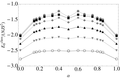
Figure 2: Ground state energy of the classical spin system as a function of the frustration parameter $\alpha$ (flux per plaquette divided by $2\pi$) for different Zeeman fields $h/JS=0,0.5,1,1.5,2$ and 2.5 (from top to bottom). The energy is symmetric around the point $\alpha=1/2$.

The classical ground states are obtained by using the Metropolis algorithm. For rational values of the frustration parameter $\alpha=p/q$, the Monte Carlo simulations are done on $nq\times nq$ lattices with periodic boundary conditions. In most cases, we find that the periodicity of the ground state is $q\times q$. However, we also find ground states with the periodicity $2q\times 2q$ in some cases. The ground-state energies as functions of the flux through a plaquette are shown in Fig. 2.

We can also examine the vortex pattern in these ground states. The current on the bond joining sites $i$ and $j$ is given by: $I_{ij}=(JS^{2}/\hbar)\sin\Theta_{i}\sin\Theta_{j}\sin\left(\Phi_{i}-\Phi_{j}+\phi_{ij}\right)$. The circulation of these currents around each plaquette gives the vortex patterns. These are shown for $\alpha=1/2,1/3$, and $1/4$ in Figs. 3 and 4.

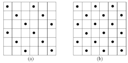
Figure 3: Vortex patterns for (a) $\alpha=1/3$ and (b) $\alpha=1/2$ (chequerboard configuration), with $\alpha$ being the flux per plaquette in units of $2\pi$. For $\alpha=1/3$ there are $2q=6$ degenerate states (vortices can be on three different $3\times 3$ sublattices and along both diagonals). For $\alpha=1/2$ there are two degenerate states with vortices at one or the other diagonal.

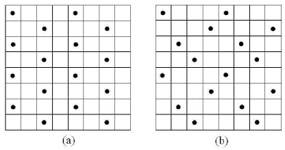
Figure 4: Vortex patterns for two ground states at $\alpha=1/4$ and $h=0$. (a) Current pattern periodic on $4\times 4$ square, phase pattern periodic on $8\times 8$ square. (b) Current and phase patterns periodic on $4\times 4$ squares.

In case of a zero Zeeman field $h=0$, the classical Hamiltonian (8) has been studied extensively in the context of Josephson junction arrays in the presence of a perpendicular magnetic field Halsey ; Straley ; Teitel . Halsey Halsey showed that, for simple fractions in the range $1/3\leq\alpha\leq 1/2$ (e.g., $\alpha=1/2,1/3,2/5,3/7,3/8$), the ground states have a constant current along diagonal staircases. Our results for $h=0$ agree with these previous studies. For a general nonzero Zeeman field, the ground states we found for $\alpha=1/2$ and $1/3$ also have currents in diagonal staircases. We cannot obtain analytic generalization of the Halsey solution for the case of finite $h$. We find the ground states by using the Metropolis algorithm. At finite $h$, the phase patterns for $\alpha=1/2$ and $\alpha=1/3$ are similar to the phase patterns for the Halsey states at $h=0$ but $S^{z}$ has spatial variation around a finite average.

The Halsey analysis does not cover cases when $\alpha<1/3$. At $\alpha=1/4$ and $h=0$ we find two distinct ground state configurations (Fig. 4) with the same energy in the agreement with previous results Straley ; Teitel ; Kasamatsu . For both configurations, the current patterns are periodic on $4\times 4$ square. However, the phase patterns do not have the same periodicity: it is $8\times 8$ periodic in the configuration shown in Fig. 4 (a) but $4\times 4$ in Fig. 4 (b). We find states of the form [Fig. 4 (b)] for general $h$ when simulations are done on $4\times 4$ lattices with periodic boundary conditions. Simulations done on larger $4n\times 4n$ lattices at nonzero $h$ give states that contain elements of both structures separated by domain walls. Similar results were found by Kasamatsu Kasamatsu .

IV Excitation Spectrum

In this section, we compute the excitations of the system using the spin-wave theory. Quantum effects are incorporated in the problem by considering finite values of $S$. We will perform an expansion in powers of the parameter $1/S$ and keep only the terms of the lowest order in $1/S$ in the Hamiltonian. Even though we are interested in $S\sim$ O(1), the large-$S$ approach is in some cases justified due to the good convergence of the perturbative series Canali ; Igarashi ; Chubukov ; Kollar ; Bernardet . Spin-wave approximation relies on an assumption that the introduction of the quantum fluctuations does not qualitatively change the nature of the ordering obtained for classical ground state. We use this approach to investigate whether the Bose condensate becomes unstable in any parameter regime.

Starting from the classical ordered state, we use the Holstein-Primakoff transformation to represent the spin flips away from the classical ground state in terms of the bosonic operators. We will keep only the quadratic terms in the final bosonic Hamiltonian. It is convenient to introduce the operators $\hat{\vec{\mathbb{S}}}_{i}$ such that $\hat{\mathbb{S}}_{i}^{x}$ direction is parallel to the classical spin direction at each site

$$\left[\begin{array}[]{c}\hat{\mathbb{S}}_{i}^{x}\\ \hat{\mathbb{S}}_{i}^{y}\\ \hat{\mathbb{S}}_{i}^{z}\end{array}\right]=\left[\begin{array}[]{ccc}\sin\Theta_{i}\cos\Phi_{i}&\sin\Theta_{i}\sin\Phi_{i}&\cos\Theta_{i}\\ -\sin\Phi_{i}&\cos\Phi_{i}&0\\ -\cos\Theta_{i}\cos\Phi_{i}&-\cos\Theta_{i}\sin\Phi_{i}&\sin\Theta_{i}\\ \end{array}\right]\left[\begin{array}[]{c}\hat{S}_{i}^{x}\\ \hat{S}_{i}^{y}\\ \hat{S}_{i}^{z}\end{array}\right],$$ (10)

and use the Holstein-Primakoff representation of these new spin operators in terms of the bosonic operators, $\hat{b}_{i}$,

$$\hat{\mathbb{S}}_{i}^{+}\equiv\hat{\mathbb{S}}_{i}^{y}+i\hat{\mathbb{S}}_{i}^{z}=(2S-\hat{b}^{\dagger}_{i}\hat{b}_{i})^{1/2}\hat{b}_{i},\qquad\hat{\mathbb{S}}_{i}^{x}=S-\hat{b}^{\dagger}_{i}\hat{b}_{i}.$$ (11)

Note that a gauge transformation corresponds to a rotation of the spin $\vec{S}$ around the $z$ axis. Since these new spin variables are aligned with the classical spin configuration (whatever the choice of gauge), the new spin $\vec{\mathbb{S}}$ is invariant under such rotation. Therefore, the bosonic operators, $\hat{b}_{i}$, are gauge invariant.

Under assumption that the zero-point fluctuations are small so that the average number of spin flips at each site is small compared to $S$, we can approximate $[1-\hat{b}^{\dagger}_{i}\hat{b}_{i}/(2S)]^{1/2}$ as unity. The resulting Hamiltonian, to order O($S^{0}$), is

$$\hat{H}\simeq E^{\rm class}_{0}+\sum_{\langle ij\rangle}\left(A_{ij}^{-}\hat{b}_{i}\hat{b}_{j}-A_{ij}^{+}\hat{b}_{i}\hat{b}_{j}^{\dagger}+{\rm H.c.}\right)+\sum_{i}C_{i}\hat{b}_{i}^{\dagger}\hat{b}_{i},$$ (12)

with

$$A_{ij}^{\pm} = \frac{JS}{2}\left[(\cos\Theta_{i}\cos\Theta_{j}\pm 1)\,c_{ij}\pm i(\cos\Theta_{i}\pm\cos\Theta_{j})\,s_{ij}\right],$$

$$C_{i} = JS\sin\Theta_{i}\sum_{j=i+\delta}\sin\Theta_{j}c_{ij}+h\cos\Theta_{i}$$ (13)

where $c_{ij}=\cos(\Phi_{i}-\Phi_{j}+\phi_{ij})$, $s_{ij}=\sin(\Phi_{i}-\Phi_{j}+\phi_{ij})$ and $E^{\rm class}_{0}$ is the ground-state value of the classical energy [Eq. (8)]. Note that all the coefficients in this Hamiltonian are gauge invariant, confirming our above conclusion that the bosonic operators, $\hat{b}_{i}$, are gauge invariant.

This Hamiltonian also reduces correctly to the case of $h>h_{c}$ (i.e., $\Theta_{i}=0$) when there is no need for realigning the axis of quantization [Eq. (10)]. In that case, the “anomalous” terms $\hat{b}\hat{b}$ and $\hat{b}^{\dagger}\hat{b}^{\dagger}$ in the Hamiltonian vanish. Then, the spin excitations are described by a tight-binding model with magnetic flux through the plaquettes:

$$\hat{H}_{h\geq h_{c}}\simeq-hNS-JS\sum_{\langle ij\rangle}\left(e^{i\phi_{ij}}\hat{b}_{i}\hat{b}_{j}^{\dagger}+{\rm H.c.}\right)+h\sum_{i}\hat{b}_{i}^{\dagger}\hat{b}_{i}.$$ (14)

This is diagonalized by the Hofstadter solution Hofstadter . The excitation spectrum has an energy gap of $h-h_{c}$ and the ground state corresponds to a vacuum of these excitations, i.e., there are no zero-point fluctuations in the ground state.

For lower Zeeman fields ($h<h_{c}$), Hamiltonian (12) containing the anomalous terms will have zero-point fluctuations which reduce the magnetization from the classical value. In the language of the original bosons, the fluctuations would deplete the condensate. The Hamiltonian can be diagonalized by a generalized Bogoliubov transformation,

$$\hat{b}_{i}=\sum_{m}\left(u_{im}\hat{\alpha}_{m}+v^{*}_{im}\hat{\alpha}^{\dagger}_{m}\right)\;,\quad\hat{b}^{\dagger}_{i}=\sum_{m}\left(v_{im}\hat{\alpha}_{m}+u^{*}_{im}\hat{\alpha}^{\dagger}_{m}\right)$$ (15)

for $m=1,\ldots$, $I$ for a lattice of $I$ sites. To ensure that the new operators $\hat{\alpha}_{m}$ obey bosonic commutation relations, we require the matrices $\mathbf{u}$ and $\mathbf{v}$ to obey: $\mathbf{u}\mathbf{u}^{\dagger}-\mathbf{v}\mathbf{v}^{\dagger}=\mathbf{1}$ and $\mathbf{u}\mathbf{v}^{\rm T}-\mathbf{v}\mathbf{u}^{\rm T}=\mathbf{0}$. To obtain a diagonalized Hamiltonian in terms of these new operators, we can write the part of the Hamiltonian (12) quadratic in the bosonic operators as $\hat{H}=\hat{c}^{\dagger}M\hat{c}$, where $M$ is a $2I\times 2I$ matrix and $\hat{c}=(\mathbf{b},\mathbf{b}^{\dagger})$ with $\mathbf{\hat{b}}=(\hat{b}_{1},\hat{b}_{2},...)$. Then, it can be shown that Hamiltonian (12) is diagonalized into the form

$$\hat{H}=E_{0}+\sum_{m}\epsilon_{m}\hat{\alpha}^{\dagger}_{m}\hat{\alpha}_{m}$$ (16)

with eigenenergies $\epsilon_{m}$ if we solve the eigenvalue problem,

$$\left(M-\frac{\epsilon}{2}\Sigma_{z}\right)q=0.$$ (17)

where $q_{m}=(u_{1m},\ldots,u_{Nm},v^{*}_{1m},\ldots,v^{*}_{Nm})$ contains the coefficients of the Bogoliubov transformation and $\Sigma_{z}=\left\{\left\{\mathbf{1},\mathbf{0}\right\},\left\{\mathbf{0},\mathbf{-1}\right\}\right\}$.

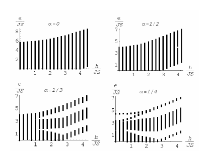
Figure 5: Low energy excitation spectrum as a function of the Zeeman field $h$ for $60\times 60$ lattices with periodic boundary conditions for frustration $\alpha=0,1/4,1/3$ and $1/2$. Critical values $h_{c}$ are: $h_{c}(\alpha=0)=4$, $h_{c}(\alpha=1/4)=2.828$, $h_{c}(\alpha=1/3)=2.732$ and $h_{c}(\alpha=1/2)=2.828$. Above $h_{c}$, the spectrum has a finite energy gap. The spectrum is gapless for $h<h_{c}$ indicating long-range order in the system.

We computed the spectrum for $60\times 60$, $120\times 120$ and $240\times 240$ lattices with periodic boundary conditions, using the classical ground states from our Monte Carlo simulations discussed in the previous section. Our results for $60\times 60$ lattices and the frustration parameters $\alpha=$ 0, 1/2, 1/3, and 1/4 are shown in Fig. 5. Our result for $\alpha=1/4$ is calculated using the $4\times 4$ periodic classical ground state presented in Fig. 4(b).

As can be seen in Fig. 5 at $h<h_{c}(\alpha)$, the spectrum is gapless. The low-energy excitations are the Goldstone modes related to the spontaneous symmetry breaking of the global rotation symmetry in the $xy$-plane in spin space. In other words, the spin system has long-range magnetization in the $xy$ plane in spin space. We can use $\langle S^{+}_{i}\rangle$ as the order parameter. In the language of the original bosonic model, this corresponds the breaking of U(1) symmetry due to Bose condensation. Above $h_{c}$, there is no symmetry breaking and we see an energy gap in the system proportional to $h-h_{c}$ as discussed above.

The ground-state energy $E_{0}$ [Eq. (16)] can be written as $E^{\rm class}_{0}+\Delta E_{0}$, where $\Delta E_{0}=\Delta+\sum_{m}\epsilon_{m}/2$ is a quantum correction to the classical ground-state energy [Eq. (8)] with $\Delta=-JS\sum_{\langle ij\rangle}\cos(\Phi_{i}-\Phi_{j}+\phi_{ij})$ for $h=0$ and $-h\sum_{i}1/(2\cos\Theta_{i})$ for $h\neq 0$. This quantum correction is of order $S^{0}$ while the classical energy is of order $S$ and so the fractional change is small in the large-$S$ limit. We calculate the relative corrections $\Delta E_{0}/E^{\rm class}_{0}$ for several lattice sizes ($60\times 60$, $120\times 120$, $240\times 240$) and extrapolate results to the thermodynamic limit shown in Fig. 6. As can be seen, the quantum correction decreases to zero as the Zeeman field $h$ approaches the critical value $h_{c}$. Above $h_{c}$, the ground state is the classical ground state containing no zero-point fluctuations.

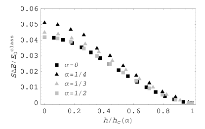
Figure 6: Quantum correction to the ground-state energy as a function of $h/h_{c}(\alpha)$ for $\alpha=0,1/2,1/3$ and $1/4$. $h_{c}(\alpha)$ is the critical value of the Zeeman field $h$ for a given frustration parameter $\alpha$.

V Density Matrix

In this section, we will examine ODLRO in the density matrix Yang ; Penrose . Consider first the case without a vector potential. A macroscopically large eigenvalue of the density matrix $\rho_{ji}$ signals the existence of Bose-Einstein condensation for our boson problem. Since we are considering a lattice system above half filling, it is more meaningful to consider the condensation of vacancies because this is the most appropriate description as $h$ approaches $h_{c}$. (For the two-species model with counterflow superfluidity, we are considering the condensation of the minority species.) The hole density matrix is defined as $\rho^{\rm h}_{ji}=\langle a_{i}a^{\dagger}_{j}\rangle$. The existence of a macroscopic eigenvalue, $N_{0}$, corresponds to Bose-Einstein condensation. The sum of all non-macroscopic eigenvalues gives the number of holes not in condensate and we can define the fractional condensate depletion as the ratio of the non-macroscopic sum to the total number of holes $N_{\rm h}$ which is the trace of the density matrix.

In the analog of the easy-plane magnet, we should study the spin-spin correlation function for the spin components in the $xy$ plane: $\rho_{ji}=\langle\hat{S}_{i}^{-}\hat{S}_{j}^{+}\rangle$. ODLRO corresponds to a non-zero $xy$ magnetization which is the analog of Bose condensation. In the large-$S$ limit, $\rho_{ji}/2S$ is the analog of the bosonic hole density matrix $\rho^{\rm h}_{ji}$ for $h$ close to $h_{c}$.

The macroscopic eigenvalue for our spin-spin correlation function is, to the leading order in $S$, given by the classical value $N_{0}^{\rm class}=\sum_{i}(m^{xy}_{i})^{2}$, where $\vec{m}^{xy}_{i}$ is the classical value of the magnetization at site $i$. We present below our results for condensate and the depletion of the condensate, i.e., zero-point fluctuations which decrease the magnetization in the ground state.

The above discussion needs to be modified in the presence of a vector potential because the density matrices, $\rho$ and $\rho^{\rm h}$, are not gauge-invariant quantities: $\rho_{ji}\rightarrow e^{i(\chi_{i}-\chi_{j})}\rho_{ji}$ under the gauge transformation [Eq. (6)]. However, we can construct gauge-invariant analogs. Moreover, the eigenvalues of $\rho$ and $\rho^{\rm h}$ are gauge invariant even though the corresponding eigenvectors are not. Consider first the spin-spin correlation function in the ground state

$$\rho_{ji} = \langle\hat{S}_{i}^{-}\hat{S}_{j}^{+}\rangle=\rho_{ji}^{\rm class}+\delta\rho_{ji}$$

$$\rho_{ji}^{\rm class} = \psi^{*}_{i}\psi_{j}\quad\mbox{with}\quad\psi_{i}=Se^{i\Phi_{i}}\sin\Theta_{i}$$ (18)

where $\rho_{ji}^{\rm class}$ is the classical value of the density matrix (of order $S^{2}$) and $\psi_{i}$ is the classical value of the order parameter (of order $S$) $\langle\hat{S}_{i}^{+}\rangle$. The order parameter itself is reduced by quantum fluctuations,

$$\langle\hat{S}_{i}^{+}\rangle=\psi_{i}(1-\Delta_{i})\,,\quad\Delta_{i}=\frac{1}{S}\sum_{m}|v_{im}|^{2}.$$ (19)

The correction $\delta\rho$ to the density matrix is given by:

$$\delta\rho_{ji}\simeq-\rho^{\rm class}_{ji}(\Delta_{i}+\Delta_{j})+\frac{S}{2}e^{i(\Phi_{j}-\Phi_{i})}\sum_{n}q_{jn}^{*}q_{in}$$ (20)

where $q_{in}=u_{in}+v_{in}+\cos\Theta_{i}(v_{in}-u_{in})$, with $u_{in}$ and $v_{in}$ being the coefficients for the Bogoliubov transformation [Eq. (15)]. This density matrix is not invariant under a gauge transformation. We obtain a gauge-invariant version of the density matrix by expressing it with respect to a gauge-covariant basis. The most natural basis is the basis formed by the eigenvectors of the classical density matrix $\rho^{\rm class}$. The eigenvector corresponding to the largest eigenvalue is simply $\psi_{i}$,

$$\sum_{i}\rho_{ji}^{\rm class}\psi_{i} = N_{0}^{\rm class}\psi_{j}\quad\mbox{with}$$

$$N_{0}^{\rm class}=\sum_{i}|\psi^{*}_{i}\psi_{i}|^{2} = S^{2}\sum_{i}\sin^{2}\Theta_{i}$$ (21)

where $N_{0}^{\rm class}$ is simply the classical value of the sum of the square of the $xy$ magnetization ($m_{xy}^{2}$) on each site. It is on the order of $NS^{2}$ at $h=0$ and tends to zero as $h$ reaches $h_{c}$. All the other eigevectors of $\rho^{\rm class}$ have eigenvalues of zero. Using an orthonormal set of these eigenvectors as columns for a unitary matrix $U$, we can construct a unitary transformation for the density matrix ($\rho\rightarrow\tilde{\rho}$, etc.),

$$\tilde{\rho}=U^{\dagger}\rho U=\tilde{\rho}^{\rm class}+\delta\tilde{\rho}\,.$$ (22)

where $\tilde{\rho}^{\rm class}=\mbox{diag}(N_{0}^{\rm class},0,\ldots,0)$. Under the gauge transformation [Eq. (6)], all the eigenvectors of $\rho_{ji}$ pick up a phase change, e.g., $\psi_{i}\rightarrow e^{-i\chi_{i}}\psi_{i}$ so that $U_{ij}\rightarrow e^{-i\chi_{i}}U_{ij}$. It is easy to check that this compensates for the phase change in $\rho_{ji}$ so that $\tilde{\rho}_{ij}\rightarrow\tilde{\rho}_{ij}$. Consequently, all the quantities obtained from the matrix $\tilde{\rho}$ are gauge-invariant and therefore physically meaningful. In this section, we calculate the effect of quantum fluctuations on the density matrix. This requires only the eigenvalues of $\tilde{\rho}$. They are in fact the same as the eigenvalues of $\rho$ because the two density matrices are related by a unitary transformation.

We will now present our numerical results. First of all, we present the classical solution for the number of atoms in the condensate, $N_{0}^{\rm class}$, as given by Eq. (V). This is shown in Fig. 7. We see that this decreases to zero as $h$ is increased to $h_{c}(\alpha)$.

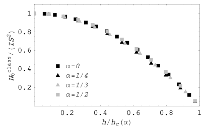
Figure 7: The condensate density per site, $N_{0}^{\rm classical}/I$, in the classical limit for $\alpha=0,1/4,1/3,1/2$. ($I=$ number of lattice sites.) $h_{c}(\alpha)$ is the critical value of the Zeeman field $h$ for a given frustration parameter $\alpha$.

Next, we compute the quantum corrections to the classical solution. In the large-$S$ expansion, these corrections are small and the leading corrections are of order $1/S$ compared to the classical limit. We have computed this leading-order correction and present results in terms of the correction to the classical limits as fractions of the classical solution.

We can exploit the large-$S$ expansion to compute the eigenvalues of the density matrix. We start with calculating the quantum correction to the non-degenerate macroscopic eigenvalue, $N_{0}$. Since $\rho_{ji}^{\rm class}$ is larger than $\delta\rho_{ji}$ by an order in $S$, we can calculate the eigenvalues of $\rho$ by treating $\delta\rho$ in perturbation theory. The first-order correction to $N_{0}$ is then given by

$$\Delta N_{0}=\frac{1}{N_{0}^{\rm class}}\sum_{ij}\psi_{i}^{*}\,\delta\rho_{ij}\,\psi_{j}=\delta\tilde{\rho}_{11}$$ (23)

if the first basis vector for $\delta\tilde{\rho}$ is chosen to be the one corresponding to the classical solution $\psi$. This correction is of order $S$, as opposed to order $S^{2}$ for the classical value. Our results for $\Delta N_{0}$ as a fraction of $N_{0}^{\rm class}$ are shown in Fig. 8. We see that the reduction in $N_{0}$ is largest at $h=0$ and decreases to zero at the critical fields $h_{c}(\alpha)$. The vanishing of quantum corrections as $h\rightarrow h_{c}$ ($\Theta_{i}\rightarrow 0$) can be seen directly from the coefficients $A^{-}$ of the anomalous terms in Hamiltonian (12) which are responsible for the zero-point fluctuations in the ground state.

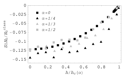
Figure 8: Quantum correction $\Delta N_{0}$ to the the macroscopic eigenvalue of the density matrix as a function of $h/h_{c}(\alpha)$ for $\alpha=0,1/4,1/3$ and $1/2$. Results have been extrapolated to the thermodynamic limit ($L\rightarrow\infty$). $h_{c}(\alpha)$ is the critical value of the Zeeman field $h$ for a given frustration parameter $\alpha$.

We can also calculate the sum of the non-macroscopic eigenvalues, $N_{\rm out}$. This corresponds to the condensate depletion in the original boson problem. In the $S\rightarrow\infty$ limit for a lattice with $I$ sites, the $I-1$ non-macroscopic eigenvalues are all zero. The first-order quantum corrections can be obtained using degenerate perturbation theory — we can obtain the eigenvalues as the eigenvalues of the $(I-1)$-dimensional submatrix $\delta\tilde{\rho}_{ji}$ for $i,j=2,\ldots,I$ which excludes the macroscopically occupied state. The sum of these eigenvalues is simply the trace of the submatrix:

$$N_{\rm out}=\sum_{i\neq 1}\delta{\tilde{\rho}}_{ii},$$ (24)

Again, $N_{\rm out}\propto S$ is one order smaller in $S$ than $N^{\rm class}_{0}$. We find that, just as classical condensate density ($N_{0}^{\rm class}/I$) vanishes as $h\to h_{c}(\alpha$), the out-of-condensate number, $N_{\rm out}$, also vanishes as $h\to h_{c}(\alpha)$. However, the ratio of the two quantities remains finite. This ratio, $N_{\rm out}/N^{\rm class}_{0}$, is the fractional depletion of the condensate. This quantity is one of interest in experiments which measure the degree of Bose-Einstein condensation by observing the time of flight of expanding condensates. Our results for this fractional depletion $N_{\rm out}/N^{\rm class}_{0}$, rescaled by $S$, are shown in Fig. 9.

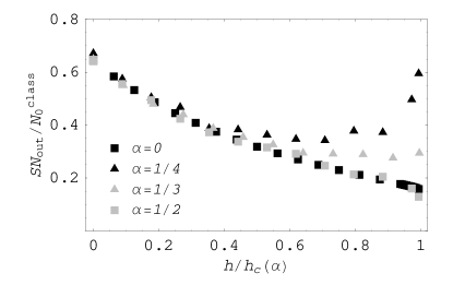
Figure 9: Fractional depletion $N_{\rm out}/N^{\rm class}_{0}$ for $\alpha=0,1/4,1/3$ and $1/2$ and as a function of $h/h_{c}(\alpha)$. $h_{c}(\alpha)$ is the critical value of the Zeeman field $h$ for a given frustration parameter $\alpha$. Results have been extrapolated to the thermodynamic limit ($L\rightarrow\infty$).

The occupation of these non-macroscopic modes is also due to the anomalous terms in the Hamiltonian. This again should vanish as $h\rightarrow h_{c}$. However, Fig. 9 shows that the occupation remains a finite fraction of $N^{\rm class}_{0}$ even at the critical field $h_{c}$. In terms of the original boson model, this result suggests that condensate depletion remains a finite fraction of the total number of holes even as the hole density decreases to zero at $h_{c}$. Our results at zero frustration agrees with previous workBernardet ; Hen .

We observe that this fractional depletion decreases monotically as we increase the Zeeman field $h$ from zero to $h_{c}$ for $\alpha=0$ and 1/2. For $\alpha=1/3$, the fractional depletion appears to have zero slope as a function of $h$ near $h_{c}$. Interestingly, for $\alpha=1/4$, the relative depletion becomes a non-monotonic function of the Zeeman field — the fractional depletion increases when $h_{c}$ is approached. In fact, if we formally set $S=1/2$, the condensate depletion even reaches unity before $h$ reaches $h_{c}$. As we will see in the next section, this change in behavior for $\alpha=1/4$ is also seen in the superfluid fraction. We discuss this further in our concluding remarks.

We note that $N_{\rm out}\neq-\Delta N_{0}$. In other words, the trace of the density matrix changes due to quantum fluctuations. This means that, in the quantum magnet, there is more than one possible measure of “condensation” in the ground state. The discrepancy can be traced to the quantum fluctuations for $S^{z}$ at each site: $\mbox{Tr }\rho=\sum_{i}\langle\hat{S}^{+}_{i}\hat{S}^{-}_{i}\rangle=\sum_{i}[S(S+1)-\langle(\hat{S}^{z}_{i})^{2}\rangle+\langle\hat{S}^{z}_{i}\rangle]$. For $S=1/2$, this is simply $\sum_{i}(1/2+\langle\hat{S}^{z}_{i}\rangle)$, corresponding to the total boson number in the original model which is a conserved quantity. However, for any $S>1/2$, the mean-square fluctuation in the local $z$-component will alter the total trace of the density matrix. In other words, this is an artifact of our large-$S$ generalization of the model. In the above, we have compared $N_{\rm out}$ with the macroscopic eigenvalue $N_{0}\simeq N^{\rm class}_{0}$. Strictly speaking, in order to discuss the depletion of the hole condensate in the original boson model, we should use the analogue for the hole density matrix and then divide the number of holes in the system. As discussed above, the correspondence is simple near $h_{c}$: we should consider $N_{\rm out}/2S$ compared to $\sum_{i}(S-\langle\hat{S}^{z}_{i}\rangle)=S\sum_{i}(1-\cos\Theta_{i})$. This is qualitatively similar to the results plotted in Fig. 9.

VI Superfluid density

Bose-Einstein condensation can be defined in equilibrium. On the other hand, superfluidity is related to the transport properties of the system. Those two phenomena are related through the phase of the macroscopic wave function (order parameter). The superflow occurs when the phase of the wave function varies in space. In this section, we calculate the superfluid density for our system as a response to an external phase twist. The superfluid density, a characteristic quantity that describes the superfluid, measures the phase stiffness under an imposed phase variation and differs from zero only in the presence of the phase ordering. We find the superfluid fraction following the calculations of Roth and BurnettRoth and Rey et al.Rey where the superfluid density is calculated for the Bose-Hubbard model with real couplings. Our results show that the superfluid fraction is reduced in the presence of the frustration.

The superfluid density introduced by considering a change in the free energy of the system under imposed phase variations Fisher ; Roth ; Rey is equivalent to the helicity modulus Fisher which differs from zero only for ordered-phase configurations and is consequently an indicator of the long-range phase coherence of the system. The definition is also equivalent to the definition of the superfluid density in terms of the winding numbers which is used in the path-integral Monte Carlo methods Pollock ; Paramekanti ; Scalettar and to Drude weight or charge stiffness which describes d.c. conductivity Poilblanc ; Kohn ; Scalpino ; Denteneer ; Shastry .

Let us consider a system of size $L_{x}$ in the $x$ direction. One way to achieve the phase twist is to impose the twisted boundary conditions on the wave function describing the system. If we assume that the phase twist is imposed along the $x$ direction the twisted boundary conditions are

$$\Psi^{\bar{\Phi}}\left(\vec{r}_{1},...,\vec{r}_{i}+L_{x}\hat{x},...\right)=e^{i\bar{\Phi}}\Psi^{\bar{\Phi}}\left(\vec{r}_{1},...,\vec{r}_{i},...\right)$$ (25)

with respect to all coordinates of the wave function. Let us introduce a unitary transformation

$$U_{\bar{\Phi}}=e^{\sum_{i}i\chi(\vec{r}_{i})}\mbox{ }\mbox{ with }\mbox{ }\bar{\Phi}=\chi\left(\vec{r}+L_{x}\hat{x}\right)-\chi\left(\vec{r}\right).$$ (26)

The untwisted wave function which satisfies the periodic boundary conditions $\Psi(\vec{r}_{1},...,\vec{r}_{i}+L_{x}\hat{x},...)=\Psi(\vec{r}_{1},...,\vec{r}_{i},...)$ is related to the twisted wave function via the unitary transformation $U_{\bar{\Phi}}$ as $|\Psi^{\bar{\Phi}}\rangle=U_{\bar{\Phi}}|\Psi\rangle$. The Schrödinger equation for the system with twisted boundary conditions, $\hat{H}|\Psi^{\bar{\Phi}}\rangle=E^{\bar{\Phi}}|\Psi^{\bar{\Phi}}\rangle$, can then be rewritten as $\hat{H}_{\bar{\Psi}}|\Psi\rangle=E^{\bar{\Phi}}|\Psi\rangle$ where the twisted Hamiltonian is

$$\hat{H}_{\bar{\Phi}}=U_{\bar{\Phi}}^{\dagger}\hat{H}U_{\bar{\Phi}}.$$ (27)

In other words, the eigenvalues of the twisted Hamiltonian with periodic boundary conditions are the same as eigenvalues of the original Hamiltonian with twisted boundary conditions.

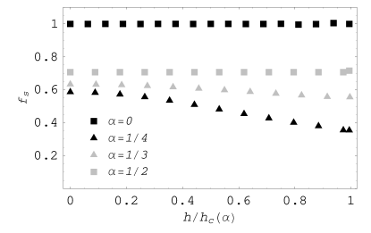
Figure 10: Superfluid density as a fraction of the classical condensate density $N_{0}^{\rm class}/I$ as a function $h/h_{c}(\alpha)$ for the frustration parameter $\alpha=0,1/4,1/3$ and $1/2$. $h_{c}(\alpha)$ is the critical value of the Zeeman field $h$ for a given frustration parameter $\alpha$.

The superfluid velocity is proportional to the order-parameter phase gradient and an additional phase variation $\chi(\vec{r})$ will change the superfluid velocity by $\Delta\vec{v}_{s}=\hbar\vec{\nabla}\chi(\vec{r})/m$ in the continuous system. When the imposed phase gradient is small so that other excitations except increase in the velocity of the superflow can be neglected the change in the ground-state energy can be approximated by $\Delta E_{g}=-\vec{P}\cdot\Delta\vec{v}_{s}+M_{s}(\Delta\vec{v}_{s})^{2}/2$, with $M_{s}=mN_{s}$ being the total mass of the superfluid part of the system. Here we choose a linear phase variation along the $\hat{x}$ direction, $\chi(\vec{r})=\bar{\Phi}x/L_{x}$. Replacing $\hbar^{2}/2m$ for the continuous system by $J/2$ for our 2D discrete lattice we obtain the following expression for the superfluid density Roth

$$n_{s}=\frac{I_{x}}{I_{y}J}\frac{\partial^{2}E_{g}(\bar{\Phi})}{\partial\bar{\Phi}^{2}}\left|{}_{\bar{\Phi}=0}\right.,$$ (28)

where $I_{x,y}=L_{x,y}/a$ with $a$ being the lattice spacing. The twisted Hamiltonian is of the same form as the untwisted one only with $\phi_{ij}$ replaced by $\phi_{ij}-\bar{\Phi}$. Under assumption that the phase twist $\bar{\Phi}\ll\pi$ we can calculate the ground state energy of the twisted Hamiltonian perturbatively. Expanding $e^{i\bar{\Phi}/L_{x}}$ up to the second order in $\bar{\Phi}$ the twisted spin Hamiltonian becomes

$$H^{\bar{\Phi}}=H+\frac{\bar{\Phi}}{I_{x}}\hat{J}_{x}-\frac{\bar{\Phi}^{2}}{2I_{x}^{2}}\hat{T}_{x},$$ (29)

where $\hat{J}_{x}=iJ\sum_{i}(e^{i\phi_{ii+x}}\hat{S}_{i}^{+}\hat{S}_{i+x}^{-}-{\rm H.c.})/2$ is the paramagnetic current operator and $\hat{T}_{x}=-J\sum_{i}(e^{i\phi_{ii+x}}\hat{S}_{i}^{+}\hat{S}_{i+x}^{-}+H.c.)/2$ corresponds to the kinetic-energy operator for the hopping in the $x$ direction. The terms in the Hamiltonian above that contain the twist angle can be treated as a small perturbation $V^{\bar{\Phi}}=\bar{\Phi}\hat{J}_{x}/I_{x}-\bar{\Phi}^{2}\hat{T}_{x}/2I_{x}^{2}$. Calculating the ground-state energy for the system with imposed small twist within the second order perturbation theory and using Eq. (28), we obtain the following expression for the superfluid density as a fraction of the condensate density, $f_{s}=I_{x}I_{y}n_{s}/N_{0}$:

$$f_{s}=-\frac{1}{N_{0}J}\left(\langle\psi_{0}|\hat{T}_{x}|\psi_{0}\rangle+2\sum_{\nu\neq 0}\frac{|\langle\psi_{\nu}|\hat{J}_{x}|\psi_{0}\rangle|^{2}}{E_{\nu}-E_{0}}\right)\mbox{ , }\mbox{ }\bar{\Phi}\ll\pi,$$ (30)

where $N_{0}\simeq N_{0}^{\rm class}$ in the large-$S$ limit and $\psi_{\nu}$ are eigenstates of original untwisted Hamiltonian with $\nu=0$ labeling the ground state. In terms of the original boson model, $N_{0}$ corresponds to the number of condensed particles or holes (for $h<0$ or $h>0$). The first term corresponds to the diamagnetic response of the condensate while the second term corresponds to the paramagnetic response involving excited states.

The results obtained for the superfluid fraction within the Bogoliubov approximation are shown in Fig. 10. The leading term due to quantum effects comes from the paramagnetic term in Eq. (30). This is of order $S^{0}$. In the absence of frustration ($\alpha=0$), the system is homogenous and the system conserves momentum. This means that the eigenstates are Bloch states corresponding to different momenta. As a result, the current matrix element in Eq. (30), which cannot couple different momenta, vanishes. Moreover, the kinetic energy in the ground state is in itself proportional to $N_{0}$. In the boson model, this means that the superfluid fraction corresponds simply to the kinetic energy per hole. This is a quantity which is independent of $h$ and so the superfluid density is the same as the condensate density in the large-$S$ limit at zero frustration. (However, $1/S$ corrections will change the result, giving a superfluid density larger than the condensate density for general $h$, but $f_{s}\to 1$ as $h\to h_{c}$.) Similarly, the current matrix element vanishes for the fully frustrated case ($\alpha=1/2$). In this case, frustration reduces the superfluid fraction in $\alpha=1/2$ case to around $70\%$. For $\alpha=1/3$ and $1/4$, an increase in the Zeeman field $h$ results in a larger reduction in the fraction $f_{s}$ at values of $h$ closer to $h_{c}(\alpha)$. That can be seen in Fig. 10 for the inhomogeneous cases of $\alpha=1/3$ and $1/4$. As for the condensate depletion, we note that the superfluid density as a fraction of the condensate density does not vanish as $h\rightarrow h_{c}$.

We also note that the superfluid density behaves differently for $\alpha=1/3$ and $1/4$ compared to $\alpha=0$ and $1/2$. The same qualitative change in behavior was observed for the condensate depletion calculated in Sec. V.

VII Conclusion

We have studied the ground state for bosonic atoms in a frustrated optical lattice by mapping the problem to a frustrated easy-plane magnet. Using a large-$S$ approach, we further introduce quantum effects under the assumption that those effects do not change qualitatively the nature of the ordering obtained for the classical ground states. We examined our results for any precursor to the non-superfluid or uncondensed states.

We have found that frustration can decrease the depletion of the condensate and the superfluid fraction. However, the fractional depletion of the condensate and the superfluid fraction remain finite for all incommensurate filling [$h<h_{c}(\alpha)$]. The behavior of the fractional condensate depletion and superfluid fraction as a function of filling has interesting behavior. We find that the cases of $\alpha=0$ and 1/2 behave differently from the cases of $\alpha=1/3$ and 1/4. Surprisingly, for the cases of smaller $\alpha$, the fractional condensate depletion becomes a nonmonotonic function of the filling, decreasing as we increase $h$ from zero but eventually increases as $h\rightarrow h_{c}$. In fact, if we formally set $S=1/2$, then the computed fractional depletion exceeds 100% for the $\alpha=1/4$ case as $h$ approaches $h_{c}$. We also have some evidence that the same behavior occurs in the $\alpha=1/6$ case for small system sizes. In other words, our results raise the possibility, for $\alpha<1/4$, of a second-order phase transition to a non-condensed state where quantum fluctuations are large enough to destroy Bose condensation. It is intriguing to note that this case does not have a Halsey-type classical ground state and in fact has two degenerate ground states with different phase patterns. One can speculate that the motion of domain walls between the two different phase patterns may contribute to a route to decondensation and/or loss of superfluidity.

Finally, we note that fractional quantum Hall states are expected when the number of vortices becomes comparable to the number of atoms or holes in the Bose-Hubbard model. In our large-$S$ theory, the boson number is proportional to $S$ and so the quantum Hall regime, if it exists in such a theory, exists only when $h-h_{c}\sim 1/S$. Therefore, one might expect the condensate depletion or the reduction in the superfluid fraction to be large as $h\rightarrow h_{c}$. We do not find this directly in our perturbative theory in $1/S$. However, our results for the fluctuations around non-Halsey-type ground states suggest that an instability to a non-condensed state may be possible.

References

- (1) N. R. Cooper, Adv. Phys. 57, 539 (2008).
- (2) R. Bhat, M. Krämer, J. Cooper, and M. J. Holland, Phys. Rev. A 76, 043601 (2007).
- (3) C. Furtado, J. R. Nascimento, and L. R. Ribeiro, Phys. Lett. A 358, 336 (2006).
- (4) J. K. Pachos, Phys. Lett. A 344, 441 (2005).
- (5) J. K. Pachos and E. Rico, Phys. Rev. A 70, 053620 (2004).
- (6) A. Kay, D. K. K. Lee, J. K. Pachos, M. B. Plenio, M. E. Reuter, and E. Rico, Opt. Spectrosc. 99,339 (2005).
- (7) D. Jaksch, and P. Zoller, New J. Phys. 5, 56 (2003).
- (8) A. S. Sørensen, E. Demler, and M. D. Lukin, Phys. Rev. Lett. 94, 086803 (2005).
- (9) J. E. Williams and M. J. Holland, Nature (London) 401, 568 (1999).
- (10) N. K. Wilkin and J. M. F. Gunn, Phys. Rev. Lett. 84, 6 (2000).
- (11) N. R. Cooper, N. K. Wilkin, and J. M. F. Gunn, Phys. Rev. Lett. 87, 120405 (2001).
- (12) E. H. Rezayi, N. Read, and N. R. Cooper, Phys. Rev. Lett. 95, 160404 (2005).
- (13) C. M. Canali, S. M. Girvin, and M. Wallin, Phys. Rev. B 45, 10131 (1992).
- (14) J. I. Igarashi, Phys. Rev. B 46, 10763 (1992).
- (15) A. V. Chubukov, S. Sahdev, and T. Senthil, J. Phys.: Condens. Matter 6, 8891 (1994).
- (16) M. Kollar, I. Spremo, and P. Kopietz, Phys. Rev. B 67, 104427 (2003).
- (17) K. Bernardet, G. G. Batrouni, J.–L. Meunier, G. Schmid, M. Troyer, and A. Dorneich, Phys. Rev. B 65, 104519 (2002).
- (18) D. K. K. Lee and J. M. F. Gunn, J. Phys.: Condens. Matter 2, 7753 (1990).
- (19) F. Pázmándi, and Z. Domanski, J. Phys. A 26, L689 (1993).
- (20) D. R. Hofstadter, Phys. Rev. B 14, 2239 (1976).
- (21) T. C. Halsey, Phys. Rev. B 31, 5728 (1985).
- (22) J. P. Straley and G. M. Barnett, Phys. Rev. B 48, 3309 (1993).
- (23) S. Teitel and C. Jayaprakash, Phys. Rev. Lett. 51, 1999 (1983).
- (24) K. Kasamatsu, Phys. Rev. A 79, 021604(R) (2009).
- (25) C. N. Yang, Rev. Mod. Phys. 34, 694 (1962).
- (26) O. Penrose and L. Onsager, Phys. Rev. 104, 576 (1956).
- (27) I. Hen and M. Rigol, Phys. Rev. B 80, 134508 (2009).
- (28) R. Roth, and K. Burnett, Phys. Rev. A 68, 023604 (2003).
- (29) A. M. Rey, K. Burnett, R. Roth, M. Edwards, C. J. Williams, and C. W. Clark, J. Phys. B 36, 825 (2003).
- (30) M. E. Fisher, M. N. Barber, and D. Jasnow, Phys. Rev. A 8, 1111 (1973).
- (31) E. L. Pollock and D. M. Ceperley, Phys. Rev. B 36, 8343 (1987).
- (32) A. Paramekanti, N. Trivedi, and M. Randeria, Phys. Rev. B 57, 11639 (1998).
- (33) R. T. Scalettar, G. Batrouni, P. Denteneer, F. Hebert, A. Muramatsu, M. Rigol, V. Rousseau, and M. Troyer, J. Low Temp. Phys. 140, 315 (2005).
- (34) D. Poilblanc, Phys. Rev. B 44, 9562 (1991).
- (35) W. Kohn, Phys. Rev. 133, A171 (1964).
- (36) D. J. Scalapino, S. R. White, and S. C. Zhang, Phys. Rev. Lett. 68, 2830 (1992); D. J. Scalapino, S. R. White, and S. Zhang, Phys. Rev. B 47, 7995 (1993).
- (37) P. J. H. Denteneer, Phys. Rev. B 49, 6364 (1994).
- (38) B. S. Shastry and B. Sutherland, Phys. Rev. Lett. 65, 243 (1990).