Extension of the Hamaneh - Taylor model using the macroscopic polarization for the description of chiral smectic liquid crystals

Abstract

Chiral smectic liquid crystals exhibit a series of phases, including ferroelectric, antiferroelectric and ferrielectric commensurate structures as well as an incommensurate $Sm-C^{*}_{\alpha}$ phase. We carried out an extension of the phenomenological model, recently presented by M. B. Hamaneh and P. L. Taylor, based upon the distorted clock model. The salient feature of this model is that it links the appearance of new phases to a spontaneous microscopic twist : i.e. an increment $\alpha$ of the azimuthal angle from layer to layer. The balance between this twist and an orientational order parameter $J$ gives the effective phase. We introduce a second orientational order parameter I which physical meaning comes from the macroscopic polarization, the effect of an applied electric is also studied. We derive new phase diagrams and correlate them to our experimental results under field showing the sequence of phases versus temperature and electric field in some compounds.

I Introduction

Chiral smectics are allowed to become ferroelectric and present a helical precession of the optical axes around the layer normal when a tilt ofthe molecules appears in the layers .Meyer et al. (1975). In the order of decreasing temperature and increasing tilt angle $\theta$, one can observe a subset of the following full sequence Chandani et al. (1989); Cady et al. (2001); Hirst et al. (2002); Olson et al. (2002) : the smectic A (Sm-A) without tilt angle ($\theta$ = 0) ; the smectic-$C^{*}_{\alpha}$ ($Sm-C^{*}_{\alpha}$) with a tilt angle $\theta$ and an azimuthal angle $\Phi$ precessing with a short incommensurate period along the layer normal ; the smectic-$C^{*}$ ($Sm-C^{*}$) with $\Phi$ precessing with a long period and an helicity sign depending on chirality, it is locally ferroelectric ($P_{S}\neq$ 0) ; the smectic-$C^{*}$ Ferri2 ($Sm-C^{*}_{Fi2}$) where $\Phi$ is periodic over four layers and has a non regular increment ($\Delta\Phi\neq 2\pi/4$) within the unit cell, the whole structure shows a long pitch helix with the same sign as the $Sm-C^{*}$, it has no macroscopic polarization ($P_{S}$ = 0) ; the smectic-$C^{*}$ Ferri1 ($Sm-C^{*}_{Fi1}$) where $\Phi$ has a non regular increment ($\Delta\Phi\neq 2\pi/3$) periodic over three layers, a long pitch helix with the opposite sign as in $SmC^{*}$, it is truly ferrielectric ($P_{S}\neq$ 0) ; the smectic-$C^{*}_{A}$ ($Sm-C^{*}_{A}$) with $\Phi$ periodic over two layers, a regular increment ($\Delta\Phi=\pi$), a long pitch helix with the opposite sign to $Sm-C^{*}$, it referred to as antiferroelectric ($P_{S}=0$) or anticlinic. Some of these phases may be missing when varying the chemical formula (tail length) Essid et al. (2004) but the order of appearance is conserved. Two of them present a macroscopic polarization, four of them a long pitch helical precession with a sign change in the middle of the sequence Devries (1951); Beaubois et al. (2000); Bitri et al. (2008). Although most of these phases present a biaxiality of the unit cell, the global structure is uniaxial because of the helical precession around the layer normal and an optical activity that can be huge results from the rotation of the biaxial structure Beaubois et al. (1999). Other nomenclatures are also adopted : $Sm-C^{*}\to Sm-C^{*}_{\beta}$, $Sm-C^{*}_{Fi1}\to Sm-C^{*}_{\gamma}$ and $Sm-C^{*}_{Fi2}\to AF$ Chandani et al. (1989); Lee et al. (1990). To characterize the different phases several experimental methods can be used : optical observations, calorimetric measurements and resonant X-ray scattering Cady et al. (2001); Hirst et al. (2002). Other subphases have been proposed Fukuda et al. (1994); Shtykov et al. (2005); Gleeson et al. (1999) but are linked to assumptions which are not accepted unanimously.

Let us briefly mention some theoretical models which have been proposed to describe the structures and behavior of chiral smectic liquid crystals. The devil’s staircase model, also called Ising model because one direction only is allowed for the azimuth, has been proposed soon after the discovery of the tilted smectic subphases by Chandani et al. Chandani et al. (1989); Fukuda et al. (1994); Matsumoto et al. (1999). It is based on the assumption that the competition between the synclinic sequence (where one layer and the following one have the same azimuth) and the anticlinic one (opposite azimuths) is at the origin of subphases which present a periodic succession of such sequences. An infinite number of phases with various ratios of synclinic versus anticlinic sequences are predicted making the so-called devil’s staircase Fukuda et al. (1994). One can define the $q_{T}$ index as the fraction S/(S+A) of synclinic ordering versus the total number. Unfortunately the same index applies to phases with different symmetries so it is simply irrelevant. This model is still supported Shtykov et al. (2005) although it has been ruled out by the results of X-ray resonant scattering experiments Mach et al. (1998).

The nearest-neighbors models are based on the definition of a quantity often called $\xi_{\alpha z}$ which measures the tilt inside a layer by the coordinates of the c-director de Gennes and Prost (1993):

$$\left(\begin{array}[]{c}\xi_{xz}\\ \xi_{yz}\end{array}\right)=\left(\begin{array}[]{c}\sin\theta\cos\Phi\\ \sin\theta\sin\Phi\end{array}\right)$$ (1)

When $\xi_{\alpha z}$ is considered as the macroscopic order parameter, it can be chosen to describe the Sm-A to Sm-C phase transition Carlsson et al. (1987); Orihara and Ishibashi (1990) as its modulus is nearly proportional to the tilt angle $\theta$. If one considers it at the layer level, defining a different $\xi_{\alpha z}^{j}$ for each layer j, it can be used to build up a local free energy taking into account the interactions between layers. Theories have been proposed which deal with these interactions by means of nearest-neighbors couplings $\xi^{j}\xi^{j+1}$ or next-nearest-neighbors $\xi^{j}\xi^{j+2}$. The form of the free energy is discrete as one has to sum up the interaction terms over all layers in the integration domain. One can find theories by Sun et al. Sun et al. (1991), Roy et al. Roy and Madhusudana (1996, 2000), Vaupotic Vaupotic and Cepic (2005). In all cases a suitable combination of coupling terms could lead to phase diagrams compatible with existing phases. Lorman has introduced linear combinations of this parameter $\xi_{\alpha z}$ over up to four layers Lorman (1996) and his treatment leads to the prediction of the well known tilted subphases except for the Sm-C${}^{*}_{\alpha}$ phase.

¿From an experimentalist’s point of view these models are of little usefulness and it is better to stay in the frame of the distorted-clock model as it gives the best description of the currently encountered phases.

I.1 The distorted-clock model

This is a purely experimental model describing the observations without ab initio theory, also called XY model because all the azimuthal directions in the layer plane are allowed. It has been derived by modeling the orientation of the molecules in the layers and then fitting the resonant scattering experiments with success. With consecutive iterations of the initial regular model Hirst et al. (2002); Mach et al. (1998), the authors have introduced some asymmetries in the azimuthal angle distribution as it is reported in figure 1. The model is still in evolution concerning the $Sm-C^{*}_{\alpha}$ phase Olson et al. (2002); Liu et al. (2007) but it is coherent and is at the base of the calculations reported here.

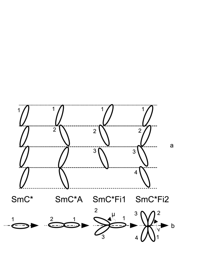
Figure 1: Schematic description of the different phases in the distorted clock model. (a) side view (same tilt angle $\theta$) period p of 1 to 4 layers, (b) top view (periodic azimuth such that $\Phi_{l+p}=\Phi_{l}+2\pi$). $\Delta\Phi=\nu$ or $\Delta\Phi=\pi-\nu$ in the $Sm-C^{*}_{Fi2}$ and $\Delta\Phi=\mu$ or $\Delta\Phi=2(\pi-\mu)$ in the $Sm-C^{*}_{Fi1}$. Arrows indicate the direction $\Phi_{0}$ taken as the origin of azimuthal angles. Any gap or overlap between molecules is due to the hand made drawing and has no physical meaning.

I.2 The Hamaneh-Taylor model

It is only recently that a new phenomenological way to describe the chiral smectic phases was proposed Hamaneh and Taylor (2004, 2005) that we call afterwards the H&T model. It is based on the balance between a short range twisting term trying to impose an increment $\alpha$ of the azimuthal angle between adjacent layers and a long range term linked to the anisotropy of curvature energy in the layer planes. They derived an order parameter $J=\langle cos2\Phi_{l}\rangle$ where the average is taken on the azimuthal angles inside the unit cell. It is non null in the phases enumerated above and associated to an energy $\eta$ J² where $\eta$ is a coefficient that describes the strength of the long-range interactions. The short order term reads $\langle cos(\Delta\Phi-\alpha)\rangle$ with $\Delta\Phi=\Phi_{l}-\Phi_{l-1}$, the elastic term is $\eta$ J² and the free energy of the sample is :

$$\frac{F}{F_{0}}=\left\langle\cos\left(\Delta\Phi-\alpha\right)\right\rangle+\eta J^{2}$$ (2)

The order of magnitude of $F_{0}$ is the electrostatic energy ($-P_{S}\cdot E_{c}$) necessary to drive at the field $E_{c}$ the phase transition to a ferroelectric phase with a polarization $P_{S}$ Hamaneh and Taylor (2004, 2005) while $\eta$ is of order unity.

This leads to a phase diagram in the ($\eta,\alpha$) plane showing the sequences of subphases which can be observed in a given liquid crystal. This model presents some limitations. First, it introduces a phase with six layers which was never observed experimentally. Second, the extent of the three layers phase is very small.

After this review we introduce in the next sections a new orientational order parameter I that will describe the contribution of the macroscopic polarization $P_{S}$ to the ordering. We present then the phases diagrams obtained from a numerical calculation. Eventually we compare the theoretical results with our experimental data obtained on several compounds

II The orientational order parameter

In H&T model it is shown clearly that the average $J=\langle cos2\Phi_{l}\rangle$ is non zero in all the phases described by the distorted clock model, by analogy we state that another average $I=\langle cos\Phi_{l}\rangle$ is also non null in the phases like $Sm-C^{*}$ and $Sm-C^{*}_{Fi1}$ which possess a macroscopic polarization. The origin $\Phi_{0}$ is such that the averages over sine functions are zero Hamaneh and Taylor (2004, 2005), it will be the azimuth $\Phi_{1}$ of the first layer except in the $Sm-C^{*}_{Fi2}$ phase where it is equal to $\Phi_{1}+\upsilon/2$. We get the following table where $\mu$ and $\upsilon$ stand for the characteristic angles of asymmetry in the Ferri phases :

	I = $\langle cos\Phi_{l}\rangle$	J = $\langle cos2\Phi_{l}\rangle$	origin $\Phi_{0}$
$Sm-C^{*}_{\alpha}$	0	0	X
$Sm-C^{*}$	1	1	$\Phi_{1}$
$Sm-C^{*}_{A}$	0	1	$\Phi_{1}$
$Sm-C^{*}_{Fi1}$	$[1+2cos\mu]/3$	$[1+2cos2\mu]/3$	$\Phi_{1}$
$Sm-C^{*}_{Fi2}$	0	$-cos\upsilon$	$\Phi_{1}+\upsilon/2$

Table 1: order parameters I and J and origin of angles in the different phases

II.1 introduction of an $I^{2}$ term in the free energy

The symmetry argument of R. Meyer .Meyer et al. (1975) stating that there exists a polarization $P$ as soon as the the layer normal $\overrightarrow{N}$ and the director $\overrightarrow{n}$ make an angle $\theta$ can be translated by introducing in the free energy the mixed product of $\overrightarrow{P}$, $\overrightarrow{N}$ and $\overrightarrow{n}$. Taking into account the table 1, the angle between $\overrightarrow{N}$ and $\overrightarrow{n}$ reads $I\theta$, so with the addition of the self energy of the polarization, one gets :

$$\Delta F_{P}=\frac{P^{2}}{2\varepsilon_{0}\chi}-CPI\theta$$ (3)

by minimizing over P one finds

$$P_{S} = \varepsilon_{0}\chi CI\theta$$

$$\Delta\tilde{F}_{P} = -\frac{P_{S}^{2}}{2\varepsilon_{0}\chi}=-\frac{\varepsilon_{0}\chi C^{2}\theta^{2}}{2}I^{2}$$

We have thus demonstrated that the term due to the macroscopic polarization $P_{S}$, present only when I is non zero, can be written $\tilde{\gamma}\theta^{2}I^{2}$ and we can add it to H&T free energy after a little bit of algebra on the orientational order parameter.

II.2 relationship between $I^{2}$ and $J^{2}$ terms.

Let us start from the de Gennes orientational order parameter in the Sm-A phase, in what follows one considers the z axis to be perpendicular to the smectic layers.

$$Q^{0}_{ij}=n_{i}n_{j}-\frac{1}{3}\delta_{ij}=\left({{\begin{array}[]{c c c}-1/3&0&0\\ 0&-1/3&0\\ 0&0&+2/3\end{array}}}\right)$$ (5)

One can build up an orientational order parameter $Q_{ij}$ for all the tilted phases of the distorted clock model by first computing for each layer, in an axis frame where z is the layer normal, the expression of $Q^{0}_{ij}$ after a tilt of the director $\vec{n}$ by an angle $\theta$. This rotation is made around an axis inside the layer such that $\Phi$ is the angle between the c-director (projection of the director $\vec{n}$ in the layer plane) and the x axis.

$$Q^{\,\theta\,\Phi}_{ij}=\left(1-\frac{3}{2}\,\sin^{2}\theta\right)\left(\begin{array}[]{c c c}-1/3&0&0\\ 0&-1/3&0\\ 0&0&+2/3\end{array}\right) + \frac{1}{2}\sin^{2}\theta\left(\begin{array}[]{c c c}\cos 2\Phi&\sin 2\Phi&\ 0\\ \sin 2\Phi&-\cos 2\Phi&\ 0\\ 0&0&\ 0\end{array}\right)$$ (12)

$$- \sin\theta\cos\theta\left(\begin{array}[]{c c c}0&0&\ \cos\Phi\\ 0&0&\ \sin\Phi\\ \cos\Phi&\sin\Phi&\ 0\end{array}\right)$$ (17)

Finally $Q_{ij}$ is computed by averaging over the unit cell of each phase. For the $Sm-C^{*}_{\alpha}$ the average over $\Phi$ is null for the second and the third matrix and there remains :

$$Q^{\alpha}_{ij}=\left(1-\frac{3}{2}\,\sin^{2}\theta\right)\left(\begin{array}[]{c c c}-1/3&0&0\\ 0&-1/3&0\\ 0&0&+2/3\end{array}\right)$$ (18)

For all other phases, one can write a general formula for $Q_{ij}$ which is a function of $\Phi_{0}$ defined in table 1 as the angle between the origin of azimuthal angles in the unit cell and the x axis. The resulting order parameter $Q_{ij}$ is unique ; it is only its expression in a given frame which depends on $\Phi_{0}$. One readily finds that the order parameters $J=\langle cos2\Phi_{l}\rangle$ and $I=\langle cos\Phi_{l}\rangle$ can be factorized in the last two matrices. For example in the $Sm-C^{*}_{Fi1}$ phase where $\Phi_{1}=\Phi_{0},\Phi_{2}=\Phi_{0}+\mu,\Phi_{3}=\Phi_{0}-\mu$, the averages in the unit cell give $\left(\cos\Phi_{1}+\cos\Phi_{2}+\cos\Phi_{3}\right)=3I\cos\Phi_{0}$, $\left(\cos 2\Phi_{1}+\cos 2\Phi_{2}+\cos 2\Phi_{3}\right)=3J\cos 2\Phi_{0}$, $\left(\sin\Phi_{1}+\sin\Phi_{2}+\sin\Phi_{3}\right)=3I\sin\Phi_{0}$, $\left(\sin 2\Phi_{1}+\sin 2\Phi_{2}+\sin 2\Phi_{3}\right)=3J\sin 2\Phi_{0}$ and so on for all the phases :

$$Q_{ij}=\left(1-\frac{3}{2}\,\sin^{2}\theta\right)\left(\begin{array}[]{c c c}-1/3&0&0\\ 0&-1/3&0\\ 0&0&+2/3\end{array}\right) + \frac{J}{2}\sin^{2}\theta\left(\begin{array}[]{c c c}\cos 2\Phi_{0}&\sin 2\Phi_{0}&\ 0\\ \sin 2\Phi_{0}&-\cos 2\Phi_{0}&\ 0\\ 0&0&\ 0\end{array}\right)$$ (25)

$$- I\sin\theta\cos\theta\left(\begin{array}[]{c c c}0&0&\ \cos\Phi_{0}\\ 0&0&\ \sin\Phi_{0}\\ \cos\Phi_{0}&\sin\Phi_{0}&\ 0\end{array}\right)$$ (30)

It is straightforward to remark that the only parameters that should be retained for building the free energy are the factorized matrix coefficients $J\,\sin^{2}\theta\sim\theta^{2}J$ and $I\sin\theta\cos\theta\sim\theta I$. So the H&T term should read $\tilde{\eta}\theta^{4}J^{2}$ and the polarization term as demonstrated above $\tilde{\gamma}\theta^{2}I^{2}$. We took advantage of this by considering that we could write the modified H&T free energy under the form :

$$\frac{F}{F_{0}} = \left\langle\cos\left(\Delta\Phi-\alpha\right)\right\rangle+\tilde{\eta}\theta^{4}J^{2}+\tilde{\gamma}\theta^{2}I^{2}$$

$$= \left\langle\cos\left(\Delta\Phi-\alpha\right)\right\rangle+\eta J^{2}+\gamma\sqrt{\eta}I^{2}$$

We then assume that the temperature dependence of the $\eta$ coefficient is due to $\theta^{4}\sim(T_{c}-T)^{2}$, where $T_{c}$ is the temperature of appearance of the tilt angle and that the coefficient $\gamma$ depends only on the compound and not on the temperature. We eventually build phase diagrams in the ($\eta,\alpha$) plane, each one for a different value of $\gamma$ taking it to be of order unity, from 0 to 1 (see e. g. figure 2). These results show that the $Sm-C^{*}$ and $Sm-C^{*}_{Fi1}$ domains grow with $\gamma$ i.e. with the permanent polarization, let us consider now what happens in the presence of an external electric which is known to induce phase transitions to polar phases Marcerou et al. (2007).

II.3 effect of electric field in the layer plane

An electric field applied to the sample always creates a small dielectric polarization proportional to it which is the same in all studied phases to first approximation. But when there is already a spontaneous polarization $P_{S}$ it will displace the energy by a term which reads roughly $-P_{S}\cdot E$. The free energy can be written by slightly modifying equation(3):

$$\Delta F_{E}=\frac{P^{2}}{2\varepsilon_{0}\chi}-CPI\theta-P\cdot E-\frac{\varepsilon_{\bot}E^{2}}{2}$$ (32)

by minimizing over P, one finds:

$$\tilde{P} = \varepsilon_{0}\chi\left(C\theta I+E\right)=P_{S}+\varepsilon_{0}\chi E$$

$$\Delta\tilde{F}_{E} = -\frac{P_{S}^{2}}{2\varepsilon_{0}\chi}-P_{S}\cdot E-\frac{\widetilde{\varepsilon}_{\bot}E^{2}}{2}$$ (33)

For a given value of the electric field, the third term $-\widetilde{\varepsilon}_{\bot}E^{2}/2$ is the same for all the phases and does not depend on the orientational order parameters I and J so we simply forget about it. The first two terms have the same order of magnitude $F_{0}\sim-P_{S}\cdot E_{c}$ and are respectively quadratic and linear versus $\theta$, so by taking $\eta$ as the main parameter we can write down :

$$\frac{F}{F_{0}}=\langle\cos\left(\Delta\Phi-\alpha\right)\rangle+\eta J^{2}+\gamma\sqrt{\eta}I^{2}+\delta\sqrt[4]{\eta}I$$ (34)

We use this expression to compute the phase diagrams in the ($\eta,\alpha$) plane, each one for a different value of $\gamma$ and $\delta$, see e.g. figure 3.

III Numerical study and phase diagrams

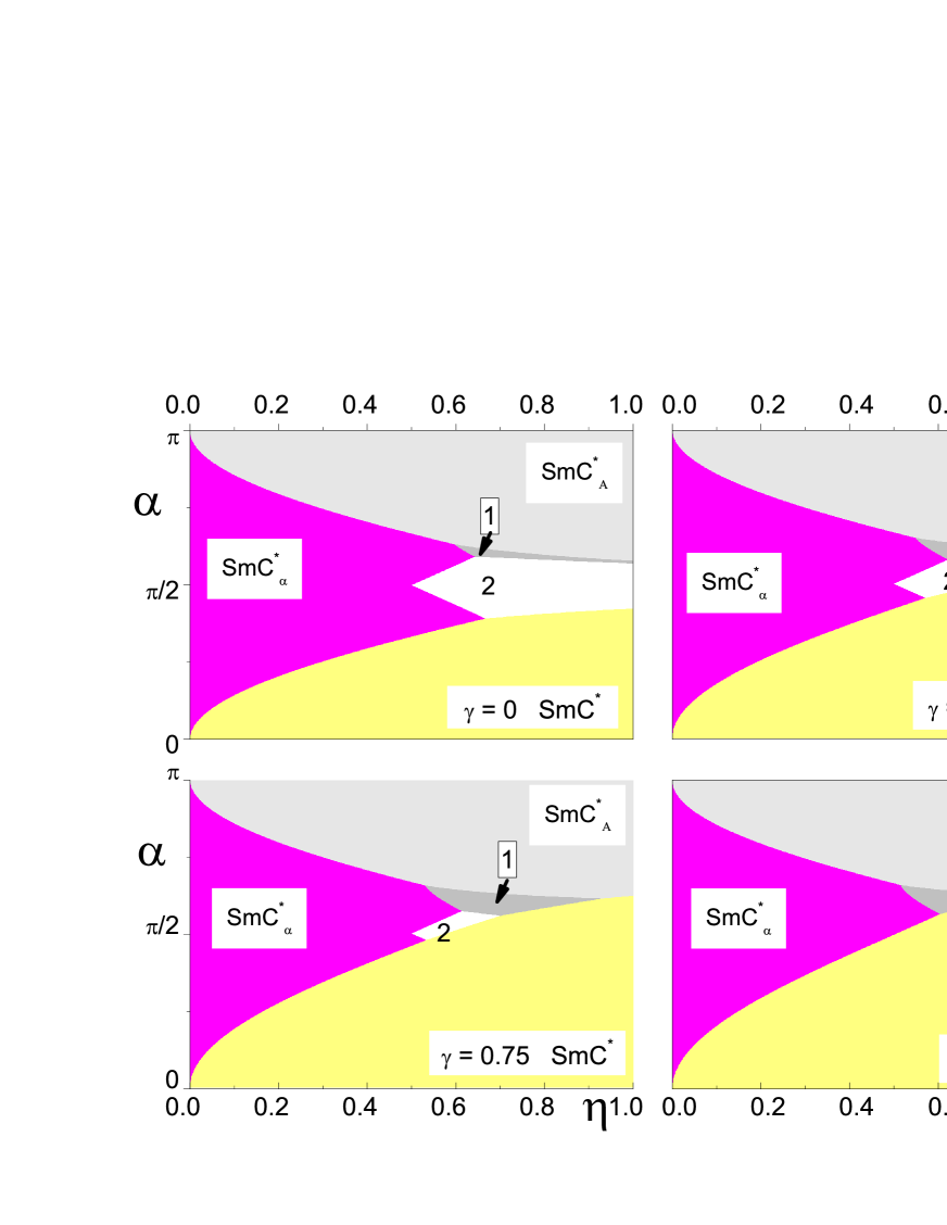
Figure 2: (Color online) Ground states diagram for $\gamma$ = 0, 0.5, 0.75 and 1. The symbols 1 and 2 stand for ferri1 and ferri2.

In the different phases of the distorted clock model represented on the figure 1, we establish at first the expression of the free energy for a given ($\eta$,$\alpha)$ by computing the order parameters I and J as well as the quantity $\langle cos(\Delta\Phi-\alpha)\rangle$ for each structure. The H&T model predicts the existence of a phase with six layers, we are going to disregard this phase on the one hand by the fact that it was never observed on the other hand because it disappears of the diagram once the term due to the polarization $P_{S}$ is added. Other structures not observed experimentally have been briefly tested like a four layers asymmetric phase which has a less favorable energy than the Ferri2 phase. Let us point out that as $F_{0}$ is negative we look for an absolute maximum of $F/F_{0}$ to get the best phase.

Figure 3: (Color online) Diagrams obtained with applied field for $\gamma=0.2$ and $\delta$ = 0, 0.2, 0.4 and 0.6. The black plain curve corresponds to an estimate of the path $\eta(\alpha)$ followed by C10F3 and the dotted line to $\eta(\alpha)$ for C7F2.

• In the $Sm-C^{*}_{\alpha}$ phase the short order term reduces to 1 while the additional terms vanish. J = 0 and I = 0 thus the free energy is F = F₀

• In the $Sm-C^{*}$ phase J = 1 and I = 1 thus

  $$\frac{F}{F_{0}}=\eta+\cos\alpha+\gamma\sqrt{\eta}+\delta\sqrt[4]{\eta}$$ (35)

• In the $Sm-C^{*}_{A}$ phase J = 1 and I = 0 thus

  $$\frac{F}{F_{0}}=\,\eta-\cos\alpha$$ (36)

• In the $Sm-C^{*}_{Fi2}$ phase $J=-\cos\upsilon$, I = 0 and by minimizing F over $\upsilon$ we find for $\eta>0.5$ that the preferred angle is such that $\sin\tilde{\upsilon}=\sin\alpha/2\eta$ and the free energy reads :

  $$\frac{F}{F_{0}}=\eta+\frac{\sin^{2}\alpha}{4\eta}$$ (37)

• In the $Sm-C^{*}_{Fi1}$ phase $J=\left(1+2\cos 2\mu\right)/3$, $I=\left(1+2\cos\mu\right)/3$ so all the terms of equation(34) must be explicited :

  $$\langle\cos(\Delta\Phi-\alpha)\rangle = \left(2\cos(\mu-\alpha)+\cos(2\mu+\alpha)\right)/3$$

  $$\eta J^{2} = \eta\left(4\cos^{2}\mu-1\right)^{2}/9$$

  $$\gamma\sqrt{\eta}I^{2} = \gamma\sqrt{\eta}\left(2\cos\mu+1\right)^{2}/9$$

  $$\delta\sqrt[4]{\eta}I = \delta\sqrt[4]{\eta}\left|2\cos\mu+1\right|/3$$ (38)

  The maximization of the energy has to be made numerically giving the preferred value of $\mu$ and $F/F_{0}$;

III.1 Computation of phase diagrams

Let us first discuss the physical meaning of these diagrams. On the x-axis one reports the values of the parameter $\eta$ that we take in mean field approximation as being the fourth power of the tilt angle $\theta$, thus the second power of the distance in temperature from the Sm-A phase - i.e. the tilt angle appears at the Sm-A to Sm-C phase transition and follows a $\sqrt{T_{c}-T}$ law. So the x-axis represents decreasing temperatures from the Sm-A at left to the right. The y-axis shows the scale of variation of the ad-hoc angle $\alpha$ from 0 to $\pi$. This parameter makes the richness of the H&T model, it means physically that due to the chirality the director wants to be twisted from layer to layer by the angle $\alpha$ and it is the balance between this tendency and a more uniform azimuthal angle distribution measured by the I and J order parameters that gives rise to the effective structures. It is remarkable that with so few parameters one can get all the structures determined experimentally before the theory was developed by H&T. One is not as usual trying to fit the experiment to a theory imposed ab initio.

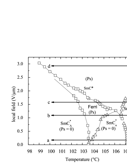
Figure 4: (E,T) phase diagram of the compound C7F2. The constant field paths a to d correspond to increasing values of the parameter $\delta$.

What we introduce in this paper are new terms linked to the polar nature of two phases in the tilted chiral smectics nomenclature, the $Sm-C^{*}$ and the $Sm-C^{*}_{Fi1}$. We express these terms as functions of the x-axis parameter, one measuring the spontaneous polarization and the other its coupling with external field. Our aim is to show that the domain filled in by these two phases will be extended in the diagram.

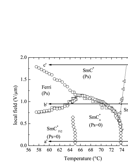
Figure 5: (E,T) phase diagram of the compound C10F3. The constant field paths a’ to c’ correspond to increasing values of the parameter $\delta$.

We first present in figure 2 some diagrams obtained for different values of $\gamma$ that correspond to the ground states without applied field. As $\gamma$ increases one notices an expansion of the domains corresponding to the $Sm-C^{*}$ and $Sm-C^{*}_{Fi1}$ phases which are the only ones with a spontaneous polarization. It is to be noticed that for $\gamma=1$ the domain corresponding to $Sm-C^{*}_{Fi2}$ has completely disappeared.

The diagram obtained with $\gamma$ = 0.2 is chosen to illustrate qualitatively (figure 3) the sequences of phases which appear for the two compounds we have studied experimentally in our group : the C10F3 and the C7F2 Essid et al. (2004); Marcerou et al. (2007); Manai et al. (2006); Essid et al. (2009).

With the applied field i.e. the parameter $\delta$ one notices also an expansion of the $Sm-C^{*}$ and $Sm-C^{*}_{Fi1}$ domains. Furthermore it appears a band corresponding to $Sm-C^{*}_{Fi1}$ in full centre of the alpha domain, this band widens gradually as $\delta$ increases.

III.2 Comparison with experiment

In the figure 3 are represented the estimated paths followed on decreasing the temperature by two compounds studied experimentally in our group : the C7F2 (dotted curve) and C10F3 (plain). The paths are unchanged in the different panels of the figure as they depend only on the temperature, the nature of the phase encountered at a given point changes as the $Sm-C^{*}_{Fi1}$ and $Sm-C^{*}$ domains grow.

The C7F2 compound shows the following ground phase sequence: $SmA\rightarrow Sm-C^{*}_{\alpha}\rightarrow Sm-C^{*}_{A}$. The corresponding path (dotted line in fig. 3) has to include the ($Sm-C^{*}_{\alpha})-(Sm-C^{*}_{Fi1})-(Sm-C^{*}_{A})$ triple point (below arrow a in fig. 4) as a very weak field reveals the $Sm-C^{*}_{Fi1}$ phase. The increase in the electric field enlarges the $Sm-C^{*}$ and $Sm-C^{*}_{Fi1}$ domains. At a certain point the path crosses the $Sm-C^{*}$ domain then the $Sm-C^{*}_{\alpha}$ and the $Sm-C^{*}_{Fi1}$ finishing in the $Sm-C^{*}_{A}$ (b and c in fig. 4). For a large enough field the $SmC^{*}$ domain will cover almost all the length of the path (arrow d).

The C10F3 compound presents at zero field the following phase sequence: $Sm-A\rightarrow Sm-C^{*}_{\alpha}\rightarrow Sm-C^{*}_{Fi2}$. For weak electric field (arrow a’ in figure 5) the sequence remains almost the same. For a higher electric field (arrow b’) the curve corresponding to the C10F3 begins in the $Sm-C^{*}$ domain then passes in the $Sm-C^{*}_{\alpha}$ before the $Sm-C^{*}_{Fi1}$ grows bigger at the expense of the $Sm-C^{*}_{Fi2}$ domain. One then encounters successively two triple points : the ($Sm-C^{*}_{\alpha})-(Sm-C^{*}_{Fi1})-(Sm-C^{*}_{Fi2})$ and the ($Sm-C^{*})-(Sm-C^{*}_{\alpha})-(Sm-C^{*}_{Fi1})$. For a strong electric field the $Sm-C^{*}$ phase is dominant (arrow c’).

III.3 Discussion

Another comparison to experiment can be made with the published values of the distortion angles $\mu$ and $\upsilon$. A. Cady et al. Cady et al. (2001) find for the $Sm-C^{*}_{Fi2}$ structure a value of $\upsilon$ of about $164^{\circ}$, Roberts et al. Roberts et al. (2005) measured the angular distortion of the $Sm-C^{*}_{Fi2}$ and $Sm-C^{*}_{Fi1}$ structures in mixtures at two temperatures, they found a value of $\upsilon$ of about $166^{\circ}$ and that of $\mu$ of about 152 to $160^{\circ}$ with no discernable dependence on temperature. Starting from our equations we made the calculation of $\upsilon$ and $\mu$ for different points from the two curves of figure 3. We found values of $\mu$ varying from 156 to $161^{\circ}$ for both compounds (under field) which is comparable to that reported by Cady, Roberts et al. Cady et al. (2001); Roberts et al. (2005). On the other hand the values we computed for the $\upsilon$ angle, about $142^{\circ}$, are slightly lower than the measured values Roberts et al. (2005); Johnson et al. (2000) but still far from the regular clock model ($\upsilon=90^{\circ}$).

We have shown that taking into account the macroscopic polarization in H&T theory one is led to an expansion of the $Sm-C^{*}$ and $Sm-C^{*}_{Fi1}$ existence domains which is correlated with the (E-T) phase diagrams we have obtained experimentally.

As noticed by H&T the translation of the theory in a quantitative way requires the knowledge of the physical path $\alpha(\eta)$ or separately $\alpha(T)$ and $\eta(T)$. What we add is the requirement for the new $\gamma$ and $\delta$ parameters which can be derived from the measurement of $P_{S}$ and E (see e.g. equation II.3). The parameter $\eta$ should be considered to be zero at the temperature $T_{c}$ where the tilt angle appears and to follow a $(T_{c}-T)^{2}$ law below. In the H&T frame it gets remarkable values at the phase boundaries like $\eta=1+\cos\alpha$ at the $Sm-C^{*}_{\alpha}$ to $Sm-C^{*}_{A}$ phase transition. So the measurement of $\alpha$ in the $Sm-C^{*}_{\alpha}$ phase is required.

Several experimental methods have been reported to measure the parameter $\alpha$, let us quote the resonant X-rays diffraction which allows to measure a periodicity ranging usually from eight to three layers in $Sm-C^{*}_{\alpha}$ with a decrease (i.e. an increase of $\alpha$) when cooling down the sample Olson et al. (2002); Mach et al. (1998); Liu et al. (2007); Cady et al. (2002). However there are a few exceptions where the periodicity varies from about ten to fifty layers ($\alpha$ is decreasing) when lowering the temperature in the assumed $Sm-C^{*}_{\alpha}$ range Hirst et al. (2002); Cady et al. (2002). This is not obviously an experiment accessible to everyone. Differential optical reflectivity has been also used to acquire the temperature variation of the helical pitch in the $Sm-C*_{\alpha}$ phase and has also shown an increase of $\alpha$ when cooling down Cady et al. (2003). Another method used by Isaert Laux et al. (1999) consists in measuring the spacing of the Friedel fringes which appear in the reflected light texture on the free surface of drops, this simple method could allow a fast measurement of $\alpha$. Finally another candidate is the gyrotropic method given by Ortega and al Ortega et al. (2003) who by a measurement of the ellipticity of eigenmodes claim to get the pitch and thus the angle $\alpha$.

IV Conclusion

In this paper we report a new successful method for the description of chiral smectic liquid crystals based on the Hamaneh - Taylor model. The introduction of the polarization and the electric field contributions give results that sound in good agreement with experiment and allow explaining the appearance under field of an intermediate ferrielectric phase. The measurement of the parameter $\alpha$ and of the polarization $P_{S}$ should allow to trace the paths followed by a given compound in the $(\eta,\alpha)$ plane. In the future we plan to introduce the helicity and its sign evolution in the phase sequence.