Time Variable Cosmological Constant from Renormalization Group Equations

Abstract

In this paper, a time variable cosmological constant (CC) from renormalization group equations (RGEs) is explored, where the renormalization scale $\mu^{2}=R^{-2}_{CC}=Max(\dot{H}+2H^{2},-\dot{H})$ is taken. The cosmological parameters, such as dimensionless energy density, deceleration parameter and effective equation of state of CC etc, are derived. Also, the cosmic observational constraints are implemented to test the model’s consistence. The results show that it is compatible with cosmic data. So, it would be a viable dark energy model.

TP-DUT/2009-06

I Introduction

Cosmological constant (CC) is a long standing issue in cosmology and physics. It was first introduced by Einstein to realize a static universe about a century ago. However, it was found that this space-time was unstable and not consistent with observed cosmological expansion. Recently, CC returns to cosmology as a natural candidate to dark energy to explain recent cosmic observation that our universe is undergoing an accelerated expansion firstly deduced from observational results of type Ia supernovae ref:Riess98 ; ref:Perlmuter99 . In the context of quantum field theory (QFT), CC has relations with the vacuum or zero point energy density of quantum fields, via

$$\rho_{\Lambda}=\frac{1}{2}\int^{\Lambda}_{0}\frac{4\pi k^{2}dk}{(2\pi)^{3}}\sqrt{k^{2}+m^{2}}\approx\frac{\Lambda^{4}}{16\pi^{2}},$$ (1)

where $\Lambda\gg m$ is a UV cut-off. To balance an assumed UV cut-off $\Lambda$ and the observational smallness of CC, tremendous fine tuning is required. This is the so-called cosmological constant problem ref:ccproblem . As known, renormalization in QFT can handle the infinities, and a dependence of the renormalized constants on some energy scale $\mu$ is leaded. This renormalized scale is usually identified with external momentum or characteristic scale of the environment.

QFT in curved space-time leads to an infinite effective action or vacuum expectation values (VEV) of the energy-momentum tensors of the fields. A renormalization treatment can yield a scale-dependent or running CC and a running Newton constant. Though, the absolute values can not be calculated, the change with respect to the renormalization scale can be calculated via RGEs originating in QFT ref:RGEsQFT and quantum gravity ref:RGEsQG . In the cosmological context, it is reasonable to identify the renormalization scale with some characteristic scales of cosmology. The related investigation can be found in ref:PhDthesis , where the renormalization scale $\mu$ was given by the Hubble scale $H$, the inverse radius $R^{-1}$ of the cosmological event horizon and the inverse radius $T^{-1}$ of the particle horizon. A scaling law having decoupling behavior at low energy in ref:PhDthesis (which was extensively studied in ref:RGEsQFT ) was explored where the corresponding $\beta$-function for $\Lambda$ is

$$\mu\frac{d\Lambda}{d\mu}=A\mu^{2},$$ (2)

where $A\sim\pm M^{2}$ is determined by the masses $M$ and the spins of the fields. Assuming constant masses and $\mu_{0}\sim H_{0}$, one has ref:PhDthesis

$$\frac{\Lambda(\mu)}{\Lambda_{0}}=L_{0}+L_{1}\frac{\mu^{2}}{\mu_{0}},\quad L_{1}\sim\pm\frac{M^{2}}{M^{2}_{P}},$$ (3)

where $L_{0}=1-L_{1}$. For sub-Planckian masses $M$, $|L_{1}|\ll 1$. Then $L_{0}\sim 1$ as a model parameter can be teste by cosmic observations. Obviously, when $L_{0}=1$, the CC becomes scale independent and a real CC is recovered.

Another consideration of time variable CC can be found in ref:Horvat1 ; ref:Horvat2 ; ref:Feng ; ref:CCXU1 ; ref:CCXU2 . Following the work ref:PhDthesis , we are going to take $R^{-2}_{CC}=Max(\dot{H}+2H^{2},-\dot{H})$ as a possible candidate to a renormalization scale to investigate the evolution of our universe in this work when the Newton constant is fixed. Though, the reports of ref:noRGE have shown that the cosmology is not a RG flow where RG was checked by a massless, minimally coupled scalar with a quartic selfinteraction on a nondynamical, locally de Sitter background. But it does not preclude using the RG conventionally to relate quantities at different constant scales. So, $R^{-2}_{CC}$ can potentially be used as a renormalization scale. Here, $R^{-2}_{CC}=Max(\dot{H}+2H^{2},-\dot{H})$ is the causal connection scale for spacially flat universe ref:CaiCC . That was investigated in the context of holographic dark energy ref:CaiCC and Ricci dark energy ref:Gao ; ref:HRDConstraint . Furthermore, it was found that only the case where $R^{-2}_{CC}=\dot{H}+2H^{2}$ as an IR cut-off was consistent with the current cosmological observations when the vacuum density appears as an independently conserved energy component ref:CaiCC . However, when a time variable CC is considered these two cases must be checked over again for its coupling with cold dark matter. It is just the case that will be explored in this paper.

This paper is structured as follows. In Section II, we give a brief review of time variable CC. We will discuss the evolution of time variable CC and derive the cosmological parameters in Section III. Cosmic observational constraints are implemented in Section IV. Section V are conclusions.

II Time variable CC

The Einstein equation with a cosmological constant is written as

$$R_{\mu\nu}-\frac{1}{2}Rg_{\mu\nu}+\Lambda g_{\mu\nu}=8\pi GT_{\mu\nu},$$ (4)

where $T_{\mu\nu}$ is the energy-momentum tensor of ordinary matter and radiation. From the Bianchi identity, one has the conservation of the energy-momentum tensor $\nabla^{\mu}T_{\mu\nu}=0$, it follows necessarily that $\Lambda$ is a constant. To have a time variable cosmological constant $\Lambda=\Lambda(t)$, one can move the cosmological constant to the right hand side of Eq. (4) and take $\tilde{T}_{\mu\nu}=T_{\mu\nu}-\frac{\Lambda(t)}{8\pi G}g_{\mu\nu}$ as the total energy-momentum tensor. Once again to preserve the Bianchi identity or local energy-momentum conservation law, $\nabla^{\mu}\tilde{T}_{\mu\nu}=0$, one has, in a spacially flat FRW universe,

$$\dot{\rho}_{\Lambda}+\dot{\rho}_{m}+3H\left(1+w_{m}\right)\rho_{m}=0,$$ (5)

where $\rho_{\Lambda}=M^{2}_{P}\Lambda(t)$ is the energy density of time variable cosmological constant and its equation of state is $w_{\Lambda}=-1$, and $w_{m}$ is the equation of state of ordinary matter, for dark matter $w_{m}=0$. It is natural to consider interactions between variable cosmological constant and dark matter ref:Horvat2 , as seen from Eq. (5). After introducing an interaction term $Q$, one has

$$\dot{\rho}_{m}+3H\left(1+w_{m}\right)\rho_{m}=Q,$$ (6)

$$\dot{\rho}_{\Lambda}+3H\left(\rho_{\Lambda}+p_{\Lambda}\right)=-Q,$$ (7)

and the total energy-momentum conservation equation

$$\dot{\rho}_{tot}+3H\left(\rho_{tot}+p_{tot}\right)=0.$$ (8)

For a time variable cosmological constant, the equality $\rho_{\Lambda}+p_{\Lambda}=0$ still holds. Immediately, one has the interaction term $Q=-\dot{\rho}_{\Lambda}$ which is different from the interactions between dark matter and dark energy considered in the literatures ref:interaction where a general interacting form $Q=3b^{2}H\left(\rho_{m}+\rho_{\Lambda}\right)$ is put by hand. With observation to Eq. (7), the interaction term $Q$ can be moved to the left hand side of the equation, and one has the effective pressure of the time variable cosmological constant- dark energy

$$\dot{\rho}_{\Lambda}+3H\left(\rho_{\Lambda}+p^{eff}_{\Lambda}\right)=0,$$ (9)

where $p^{eff}_{\Lambda}=p_{\Lambda}+\frac{Q}{3H}$ is the effective dark energy pressure. Also, one can define the effective equation of state of dark energy, (for other definition, please see ref:EEoS ),

$$w^{eff}_{\Lambda} = \frac{p^{eff}_{\Lambda}}{\rho_{\Lambda}}$$ (10)

$$= -1+\frac{Q}{3H\rho_{\Lambda}}$$

$$= -1-\frac{1}{3}\frac{d\ln\rho_{\Lambda}}{d\ln a}.$$

The Friedmann equation as usual can be written as, in a spacially flat FRW universe,

$$H^{2}=\frac{1}{3M^{2}_{P}}\left(\rho_{m}+\rho_{\Lambda}\right).$$ (11)

III Evolution of Time Variable CC and Cosmological Parameters

The time variable CC and $G$ was explored in ref:PhDthesis , where the renormalization scale $\mu$ was given by the Hubble scale $H$, the inverse radius $R^{-1}$ of the cosmological event horizon and the inverse radius $T^{-1}$ of the particle horizon. In this paper, we are going to reconsider the time variable CC when $R^{-2}_{CC}=Max(\dot{H}+2H^{2},-\dot{H})$ is taken as a renormalization scale $\mu$, say $\mu^{2}=R^{-2}_{CC}$. Though the authors of ref:CaiCC have claimed the case where $R^{-2}_{CC}=\dot{H}+2H^{2}$ as an IR cut-off was consistent with the current cosmological observations when the vacuum density appears as an independently conserved energy component. For the existence of effective interaction between time variable CC and cold dark matter, the two cases must been checked over again. We name the case $\mu^{2}=\dot{H}+2H^{2}$ Model A and $\mu^{2}=-\dot{H}$ Model B.

III.1 Molde A: $\mu^{2}=\dot{H}+2H^{2}$

In this case, the time variable CC can be written as

$$\Lambda(t) = \Lambda_{0}(L_{0}+L_{1}\frac{R}{R_{0}})$$ (12)

$$= \Lambda_{0}(L_{0}+L_{1}\frac{\dot{H}+2H^{2}}{\dot{H}_{0}+2H^{2}_{0}}).$$

From the above equation, it seems the CC behaves quite like Ricci dark energy. But in fact, it is different from that for its effective interaction with cold dark matter. The corresponding vacuum energy density is

$$\rho_{\Lambda} = M^{2}_{P}\Lambda(t)$$ (13)

$$= M^{2}_{P}\Lambda_{0}(L_{0}+L_{1}\frac{\dot{H}+2H^{2}}{\dot{H}_{0}+2H^{2}_{0}})$$

$$= M^{2}_{P}\Lambda_{0}\left[L_{0}+M_{0}(\dot{H}+2H^{2})\right],$$

where $M_{0}=(1-L_{0})/(\dot{H}_{0}+2H^{2}_{0})$. For its interaction between $\rho_{\Lambda}$ and cold dark matter $\rho_{m}$, they are not conservative separately. By using the definition of dimensionless density parameters $\Omega_{m}(z)=\rho_{m}/(3M^{2}_{P}H^{2})$ and $\Omega_{\Lambda}(z)=\rho_{\Lambda}/(3M^{2}_{P}H^{2})$, one has

$$\rho_{m} = \left(\frac{1-\Omega_{\Lambda}}{\Omega_{\Lambda}}\right)\rho_{\Lambda}.$$ (14)

Then after easy algebra, the conservation Eq. (5) can be rewritten as

$$\dot{H}+\frac{3}{2}H^{2}(1-\Omega_{\Lambda})=0.$$ (15)

From Eq. (13), one has the expression of $\Omega_{\Lambda}$

$$\Omega_{\Lambda} = \frac{\Lambda_{0}}{3H^{2}}\left[L_{0}+M_{0}(\dot{H}+2H^{2})\right]$$ (16)

$$= \frac{B_{0}}{3H^{2}}+\frac{A_{0}}{3}\left(2+\frac{\dot{H}}{H^{2}}\right),$$

where $A_{0}=\Lambda_{0}M_{0}$ and $B_{0}=\Lambda_{0}L_{0}$ for convenience. Combining Eq. (15) and Eq. (16), one has

$$\left(1-\frac{A_{0}}{2}\right)\frac{\dot{H}}{H^{2}}-\frac{B_{0}}{2}\frac{1}{H^{2}}+\frac{3}{2}\left(1-\frac{2A_{0}}{3}\right)=0,$$ (17)

In terms of redshift $z$, the above Eq. (17) can be rewritten as

$$-\left(1-\frac{A_{0}}{2}\right)\frac{(1+z)}{2}\frac{d\ln E(z)}{dz}-\frac{B^{\prime}_{0}}{2}\frac{1}{E(z)}+\frac{3}{2}\left(1-\frac{2A_{0}}{3}\right)=0,$$ (18)

where $H^{2}(z)=H^{2}_{0}E(z)$ is used and $B^{\prime}_{0}=B_{0}/H^{2}_{0}$ which is a dimensionless parameter. The above differential equation has the integration

$$E(z)=\left[1-\frac{B^{\prime}_{0}}{(3-2A_{0})}\right](1+z)^{3+A_{0}/(A_{0}-2)}+\frac{B^{\prime}_{0}}{(3-2A_{0})}.$$ (19)

III.2 Model B: $\mu^{2}=-\dot{H}$

In this case, the time variable CC can be written as

$$\Lambda(t)=\Lambda_{0}(L_{0}+L_{1}\frac{\dot{H}}{\dot{H}_{0}}).$$ (20)

As done in III.1, one has the expression of $\Omega_{\Lambda}$ and differential equation of $H$

$$\Omega_{\Lambda}=\frac{\Lambda_{0}}{3H^{2}}\left(L_{0}+N_{0}\dot{H}\right),$$ (21)

$$(1-\frac{C_{0}}{2})\frac{\dot{H}}{H^{2}}-\frac{B_{0}}{2}\frac{1}{H^{2}}+\frac{3}{2}=0,$$ (22)

where $N_{0}=(1-L_{0})/\dot{H}_{0}$ and $C_{0}=\Lambda_{0}N_{0}$. Also, one can find the Hubble parameter $H(z)$ as a solution of Eq. (22) with respect to redshift $z$ as follows

$$H^{2}(z)=H^{2}_{0}\left[\left(1-\frac{B^{\prime}_{0}}{3}\right)(1+z)^{\frac{6}{2-C_{0}}}+\frac{B^{\prime}_{0}}{3}\right].$$ (23)

It is clear that $\Lambda$CDM is recovered when $C_{0}=0$, i.e. $L_{0}=1$.

III.3 Discussion

From these Friedmann equations (19) and Eq. (23), one can immediately find out that the first terms of the right hand of the equations behave like cold dark matter for $A_{0}=0$ and $C_{0}=0$ respectively, i.e. $L_{0}=1$. In these cases, the $\Lambda$CDM universe are recovered as expected in introduction. These models contain two parameters $A_{0}$($C_{0}$) and $B^{\prime}_{0}$ which can be determined by cosmic observations. If this model does not badly depart from $\Lambda$CDM universe, we can estimate the values of parameters $A_{0}$($C_{0}$) and $B^{\prime}_{0}$. It is to say $A_{0}\sim 0$($C_{0}\sim 0$) and $B^{\prime}_{0}\sim 3\Omega_{\Lambda 0}\sim 2.1$ which can be tested by cosmic observations. In terms of redshift, the deceleration parameter and effective EoS of CC can be written as

$$q = -1+\frac{(1+z)}{2}\frac{d\ln H^{2}}{dz},$$ (24)

$$w^{eff}_{\Lambda} = -1+\frac{(1+z)}{3}\left(\frac{d\ln H^{2}}{dz}+\frac{d\ln\Omega_{\Lambda}(z)}{dz}\right).$$ (25)

From Eq. (19), one can find two singularity points with parameter values of $A_{0}=2\text{ and }3/2$ respectively. The same case can be found in Eq. (23) when $C_{0}=2$. When $A_{0}=2$, the first term of left hand side of Eq. (17) vanishes. Then one has a constant Hubble parameter $H^{2}=-1/B_{0}$. For the positivity of the value of $B_{0}>0$, it does not describe a physical system. However, for $C_{0}=2$, one has $H^{2}=B_{0}/3$. Then, in this case, a de Sitter or anti de Sitter universe can be obtained. When $A_{0}=3/2$, one has $\dot{H}=2B_{0}$ which corresponds to scale factor $a(t)\sim\exp(B_{0}t^{2})$.

IV Cosmic Observational Constraints

Now, it is proper to present the constraint results by using cosmic observations: SN Ia, BAO and CMB shift parameter $R$, for the details please see Appendix A. In this work, 397 SN Ia Constitution dataset, the ratio $D_{V}(0.35)/D_{V}(0.2)$ detected by BAO and CMB $R$ from WMAP5 are used. After the calculation as described in Appendix A, the results are listed in Tab. 1.

Model	$\chi^{2}_{min}$	$\Omega_{\Lambda 0}(1\sigma)$	$A_{0}\text{ or }C_{0}(1\sigma)$	$B^{\prime}_{0}(1\sigma)$	$z_{T}(1\sigma)$	$\chi^{2}_{min}/dof$
A	$473.593$	$0.732\pm 0.021$	$(1.0\times 10^{-11})^{+0.0217}_{-0.108}$	$2.196^{+0.0780}_{-0.0833}$	$0.762^{+0.071}_{-0.069}$	$1.193$
B	$473.593$	$0.732\pm 0.021$	$(-7.011\times 10^{-10})^{+0.0292}_{-0.00703}$	$2.196^{+0.0780}_{-0.0833}$	$0.762^{+0.072}_{-0.070}$	$1.193$

Table 1: The minimum values of $\chi^{2}$ and best fit values of the parameters. Here $z_{T}$ is the transition redshift from decelerated expansion to accelerated expansion and $dof$ denotes the model degrees of freedom.

The evolution curves of $q(z)$, $w^{eff}_{\Lambda}(z)$ and dimensionless density parameters $\Omega_{m}(z)$ and $\Omega_{\Lambda}(z)$ are plotted in Fig. 1 and Fig. 2.

Figure 1: Model A: The evolution curves of $q(z)$ (left panel), $w^{eff}_{\Lambda}(z)$ (central panel) with $1\sigma$ error region and dimensionless parameters $\Omega_{m}(z)$ and $\Omega_{\Lambda}(z)$ (right panel) with respect to redshift $z$ where the best fit values are adopted.

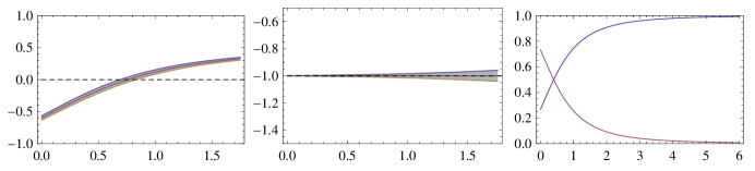
Figure 2: Model B: The evolution curves of $q(z)$ (left panel), $w^{eff}_{\Lambda}(z)$ (central panel) with $1\sigma$ error region and dimensionless parameters $\Omega_{m}(z)$ and $\Omega_{\Lambda}(z)$ (right panel) with respect to redshift $z$ where the best fit values are adopted.

Also, the contour plots of $A_{0}-B^{\prime}_{0}$ and $C_{0}-B^{\prime}_{0}$ are shown in Fig. 3 and Fig. 4.

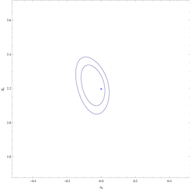
Figure 3: Model A: The contours in the planes of $A_{0}-B^{\prime}_{0}$ with $1\sigma$ and $2\sigma$ regions. The central dot denotes the best fit values of model parameters.

Figure 4: Model B: The contours in the planes of $C_{0}-B^{\prime}_{0}$ with $1\sigma$ and $2\sigma$ regions. The central dot denotes the best fit values of model parameters.

From the left panels of Fig. 1 and Fig. 2, one can easily find that our universe is undergoing accelerated expansion at late time, and the transition redshift from decelerated expansion to accelerated expansion are $z_{T}\sim 0.762$, which are consistent with other analysis results with best fit parameter values. In the early epoch, our universe is dominated by cold dark matter, that can be seen from the left and right panels of Fig. 1 and Fig. 2 where the deceleration parameter is $q\rightarrow 1/2$ (dark matter dominated) and $\Omega_{m}\rightarrow 1$ at high redshift. From the central panels of Fig. 1 and Fig. 2, one can see the effective EoS of time variable CC is almost constant $w^{eff}_{\Lambda}(z)\sim-1$. So, the universe is quasi-$\Lambda$CDM and it is not necessary to worry about the structure formation of the universe. With the best fit values of the parameters and $L_{0}=B^{\prime}_{0}/(3\Omega_{\Lambda 0})$, one obtains the mass of the fields is $M=|1-L_{0}|^{1/2}M_{P}\sim 1.490\times 10^{-8}M_{P}$ and $L_{1}\sim-2.220\times 10^{-16}$ in Model A and Model B which confirms the prediction in the introduction.

V Conclusions

In this paper, time variable cosmological constant from renormalization group equations (RGEs) is explored, where the renormalization scale $\mu^{2}=R^{-2}_{CC}=Max(\dot{H}+2H^{2},-\dot{H})$ is taken. The cosmological parameters, such as dimensionless energy density, deceleration parameter and effective EoS of CC etc, are derived. Also, the comic observational constraints are implemented to test the model’s consistence, the results are shown in Tab. 1. As investigated, with this time variable CC, the universe is undergoing an accelerated expansion at late time and a decelerated expansion at high redshift. And, the transition redshift from decelerated expansion to accelerated expansion is $z_{T}\sim 0.762$ which is consistent with other results. The effective EoS of time variable CC is almost constant $w^{eff}_{\Lambda}(z)\sim-1$. In early epoch, our universe is dominated by cold dark matter, that can be seen from the left and right panels of Fig. 1 and Fig. 2 where the deceleration parameter is $q\rightarrow 1/2$ and $\Omega_{m}\rightarrow 1$ (dark matter dominated) at high redshift. And the current cold dark matter density ratio is $\Omega_{\Lambda 0}\sim 0.732$ which is also compatible with other analysis. So, via RGEs with the renormalization scale $\mu^{2}=R^{-2}_{CC}=Max(\dot{H}+2H^{2},-\dot{H})$, time variable CC is viable. With the best fit values of the parameters and $L_{0}=B^{\prime}_{0}/(3\Omega_{\Lambda 0})$, one obtains the mass of the fields is $M=|1-L_{0}|^{1/2}M_{P}\sim 1.490\times 10^{-8}M_{P}$ and $L_{1}\sim-2.220\times 10^{-16}$ in Model A and Model B which confirms the prediction in the introduction and implies that the mass scale having relations with CC about $10^{-8}$ order of $M_{P}$.

Appendix A Cosmic Observations

A.1 SN Ia

We constrain the parameters with the 397 SN Ia Constitution dataset including $397$ SN Ia ref:Condata . Constraints from SN Ia can be obtained by fitting the distance modulus $\mu(z)$

$$\mu_{th}(z)=5\log_{10}(D_{L}(z))+\mu_{0},$$ (26)

where, $D_{L}(z)$ is the Hubble free luminosity distance $H_{0}d_{L}(z)/c$ and

$$d_{L}(z) = c(1+z)\int_{0}^{z}\frac{dz^{\prime}}{H(z^{\prime})}$$ (27)

$$\mu_{0} \equiv 42.38-5\log_{10}h,$$ (28)

where $H_{0}$ is the Hubble constant which is denoted in a re-normalized quantity $h$ defined as $H_{0}=100h~{}{\rm km~{}s}^{-1}{\rm Mpc}^{-1}$. The observed distance moduli $\mu_{obs}(z_{i})$ of SN Ia at $z_{i}$ is

$$\mu_{obs}(z_{i})=m_{obs}(z_{i})-M,$$ (29)

where $M$ is their absolute magnitudes.

For SN Ia dataset, the best fit values of parameters in a model can be determined by the likelihood analysis is based on the calculation of

$$\chi^{2}(p_{s},m_{0}) \equiv \sum_{SNIa}\frac{\left[\mu_{obs}(z_{i})-\mu_{th}(p_{s},z_{i})\right]^{2}}{\sigma_{i}^{2}}$$ (30)

$$= \sum_{SNIa}\frac{\left[5\log_{10}(D_{L}(p_{s},z_{i}))-m_{obs}(z_{i})+m_{0}\right]^{2}}{\sigma_{i}^{2}},$$

where $m_{0}\equiv\mu_{0}+M$ is a nuisance parameter (containing the absolute magnitude and $H_{0}$) that we analytically marginalize over ref:SNchi2 ,

$$\tilde{\chi}^{2}(p_{s})=-2\ln\int_{-\infty}^{+\infty}\exp\left[-\frac{1}{2}\chi^{2}(p_{s},m_{0})\right]dm_{0}\;,$$ (31)

to obtain

$$\tilde{\chi}^{2}=A-\frac{B^{2}}{C}+\ln\left(\frac{C}{2\pi}\right),$$ (32)

where

$$A=\sum_{SNIa}\frac{\left[5\log_{10}(D_{L}(p_{s},z_{i}))-m_{obs}(z_{i})\right]^{2}}{\sigma_{i}^{2}},$$ (33)

$$B=\sum_{SNIa}\frac{5\log_{10}(D_{L}(p_{s},z_{i})-m_{obs}(z_{i})}{\sigma_{i}^{2}},$$ (34)

$$C=\sum_{SNIa}\frac{1}{\sigma_{i}^{2}}\;.$$ (35)

The Eq. (30) has a minimum at the nuisance parameter value $m_{0}=B/C$. Sometimes, the expression

$$\chi^{2}_{SNIa}(p_{s},B/C)=A-(B^{2}/C)$$ (36)

is used instead of Eq. (32) to perform the likelihood analysis. They are equivalent, when the prior for $m_{0}$ is flat, as is implied in (31), and the errors $\sigma_{i}$ are model independent, what also is the case here.

To determine the best fit parameters for each model, we minimize $\chi^{2}(p_{s},B/C)$ which is equivalent to maximizing the likelihood

$${\cal{L}}(p_{s})\propto e^{-\chi^{2}(p_{s},B/C)/2}.$$ (37)

A.2 BAO

The BAO are detected in the clustering of the combined 2dFGRS and SDSS main galaxy samples, and measure the distance-redshift relation at $z=0.2$. BAO in the clustering of the SDSS luminous red galaxies measure the distance-redshift relation at $z=0.35$. The observed scale of the BAO calculated from these samples and from the combined sample are jointly analyzed using estimates of the correlated errors, to constrain the form of the distance measure $D_{V}(z)$ ref:Okumura2007 ; ref:Eisenstein05 ; ref:Percival

$$D_{V}(z)=\left[(1+z)^{2}D^{2}_{A}(z)\frac{cz}{H(z)}\right]^{1/3},$$ (38)

where $D_{A}(z)$ is the proper (not comoving) angular diameter distance which has the following relation with $d_{L}(z)$

$$D_{A}(z)=\frac{d_{L}(z)}{(1+z)^{2}}.$$ (39)

Matching the BAO to have the same measured scale at all redshifts then gives ref:Percival

$$D_{V}(0.35)/D_{V}(0.2)=1.812\pm 0.060.$$ (40)

Then, the $\chi^{2}_{BAO}(p_{s})$ is given as

$$\chi^{2}_{BAO}(p_{s})=\frac{\left[D_{V}(0.35)/D_{V}(0.2)-1.812\right]^{2}}{0.060^{2}}.$$ (41)

A.3 CMB shift Parameter R

The CMB shift parameter $R$ is given by ref:Bond1997

$$R(z_{\ast})=\sqrt{\Omega_{m}H^{2}_{0}}(1+z_{\ast})D_{A}(z_{\ast})/c$$ (42)

which is related to the second distance ratio $D_{A}(z_{\ast})H(z_{\ast})/c$ by a factor $\sqrt{1+z_{\ast}}$. Here the redshift $z_{\ast}$ (the decoupling epoch of photons) is obtained by using the fitting function Hu:1995uz

$$z_{\ast}=1048\left[1+0.00124(\Omega_{b}h^{2})^{-0.738}\right]\left[1+g_{1}(\Omega_{m}h^{2})^{g_{2}}\right],$$ (43)

where the functions $g_{1}$ and $g_{2}$ are given as

$$g_{1} = 0.0783(\Omega_{b}h^{2})^{-0.238}\left(1+39.5(\Omega_{b}h^{2})^{0.763}\right)^{-1},$$ (44)

$$g_{2} = 0.560\left(1+21.1(\Omega_{b}h^{2})^{1.81}\right)^{-1}.$$ (45)

The 5-year WMAP data of $R(z_{\ast})=1.710\pm 0.019$ ref:Komatsu2008 will be used as constraint from CMB, then the $\chi^{2}_{CMB}(p_{s})$ is given as

$$\chi^{2}_{CMB}(p_{s})=\frac{(R(z_{\ast})-1.710)^{2}}{0.019^{2}}.$$ (46)

References

• (1) A.G. Riess, et al., Astron. J. 116 1009(1998) [astro-ph/9805201].
• (2) S. Perlmutter, et al., Astrophys. J. 517 565(1999) [astro-ph/9812133].
• (3) S. Weinberg, Rev. Mod. Phys. 61 (1989) 1.
• (4) I. L. Shapiro, J. Sola, Phys. Lett. B 475 (2000) 236, hep-ph/9910462; I. L. Shapiro, J. Sola, JHEP 0202 (2002) 006, hep-th/0012227; I. L. Shapiro, J. Sola, C. Espana- Bonet, P. Ruiz-Lapuente, Phys. Lett. B 574 (2003) 149, astro-ph/0303306; C. Espana-Bonet, P. Ruiz-Lapuente, I. L. Shapiro, J. Sola, JCAP 0402 (2004) 006, hep-ph/0311171; I. L. Shapiro, J. Sola, astro-ph/0401015; I. L. Shapiro, J. Sola, H. Stefancic, JCAP 0501 (2005) 012, hep-ph/0410095; J. Grande, J. Sola and H. Stefancic, gr-qc/0604057.
• (5) M. Reuter, Phys. Rev. D 57 (1998) 971, hep-th/9605030; A. Bonanno and M. Reuter, Phys. Rev. D 65 (2002) 043508, hep-th/0106133; M. Reuter, H. Weyer, JCAP 0412 (2004) 001, hep-th/0410119.
• (6) F. Bauer, PhD thesis, [arXiv:hep-th/0610178].
• (7) P. Horava, D. Minic, Phys. Rev. Lett. 85 1610(2000).
• (8) R. Horvat, Phys. Rev. D70 087301(2004).
• (9) C.J. Feng, Phys. Lett. B 663 367(2008).
• (10) L. Xu, W. Li, J. Lu, arXiv:0905.4772 [astro-ph.CO].
• (11) L. Xu, J. Lu, W. Li, arXiv:0905.4773 [astro-ph.CO].
• (12) R. P. Woodard, Phys. Rev. Lett.101 081301(2008).
• (13) R. G. Cai, B. Hu and Y. Zhang, [arXiv:0812.4504].
• (14) C. Gao, F. Wu, X. Chen, Y.G. Shen, Phys. Rev. D 79 043511(2009) [arXiv:0712.1394].
• (15) L. Xu, W. Li, J. Lu, [arXiv:0810.4730]; X. Zhang, [arXiv:0901.2262].
• (16) B. Wang, C.Y. Lin, E.o Abdalla, Phys. Lett. B 637 357(2006); H. Kim, H.W. Lee, Y.S. Myung, Phys. Lett. B 632 605(2006); B. Hu, Y. Ling, Phys. Rev. D 73 123510(2006); W. Zimdahl, D. Pavon, [arXiv:astro-ph/0606555]; H.M. Sadjadi, JCAP 02 026(2007); M.R. Setare, E.C. Vagenas, Int. J. Mod. Phys. D 18 147(2009); Q. Wu, Y. Gong, A. Wang, J.S. Alcaniz, [arXiv:0705.1006]; J.F. Zhang, X. Zhang, H.Y. Liu, Phys. Lett. B 659 26(2008); C. Feng, B. Wang, Y. Gong, R.K. Su, [arXiv:0706.4033]; S.F. Wu, P.M. Zhang, G.H. Yang, Class. Quan. Grav. 26 055020(2009); M. A. Rashid, M. U. Farooq, M. Jamil, [arXiv:0901.3724].
• (17) J. Sola, H. Stefancic, Mod. Phys. Lett. A 21, 479(2006); J. Sola, H. Stefancic, Phys. Lett. B 624,147(2005).
• (18) M. Hicken et al., arXiv:0901.4804 [astro-ph.CO].
• (19) S. Nesseris and L. Perivolaropoulos, Phys. Rev. D 72, 123519 (2005) [arXiv:astro-ph/0511040]; L. Perivolaropoulos, Phys. Rev. D 71, 063503 (2005) [arXiv:astro-ph/0412308]; S. Nesseris and L. Perivolaropoulos, JCAP 0702, 025 (2007) [arXiv:astro-ph/0612653]; E. Di Pietro and J. F. Claeskens, Mon. Not. Roy. Astron. Soc. 341, 1299 (2003) [arXiv:astro-ph/0207332].
• (20) T. Okumura, T. Matsubara, D. J. Eisenstein, I. Kayo, C. Hikage, A. S. Szalay and D. P. Schneider, ApJ 676, 889(2008) [arXiv:0711.3640]
• (21) D. J. Eisenstein, et al, Astrophys. J. 633, 560 (2005) [astro-ph/0501171].
• (22) W.J. Percival, et al, Mon. Not. Roy. Astron. Soc., 381, 1053(2007) [arXiv:0705.3323]
• (23) J. R. Bond, G. Efstathiou, and M. Tegmark, MNRAS 291 L33(1997).
• (24) W. Hu, N. Sugiyama, Astrophys. J. 471 542(1996) [astro-ph/9510117].
• (25) E. Komatsu, et.al., Astrophys. J. Suppl. 180, 330(2009) [arXiv:0803.0547].