Monotonically convergent optimal control theory of quantum systems with spectral constraints on the control field

Abstract

We propose a new monotonically convergent algorithm which can enforce spectral constraints on the control field (and extends to arbitrary filters). The procedure differs from standard algorithms in that at each iteration the control field is taken as a linear combination of the control field (computed by the standard algorithm) and the filtered field. The parameter of the linear combination is chosen to respect the monotonic behavior of the algorithm and to be as close to the filtered field as possible. We test the efficiency of this method on molecular alignment. Using band-pass filters, we show how to select particular rotational transitions to reach high alignment efficiency. We also consider spectral constraints corresponding to experimental conditions using pulse shaping techniques. We determine an optimal solution that could be implemented experimentally with this technique.

1 Introduction

Quantum control is a field of growing interest both from the experimental and theoretical points of views [1, 2, 3]. On the experimental side, the development of pulse shaping techniques opens new ways to control atomic or molecular processes by laser fields. Many promising results have been obtained in the implementation of closed-loop control experiments (CLC) based on genetic or evolutionary algorithms (See [4, 5, 6, 7, 8] to cite a few). This setup is made of a pulse shaper controlled by the algorithm which from the results of the preceding experiments builds an improved new control field. Such algorithms lead to very efficient solutions, but have some negative points. In particular, no insight into the control mechanism is gained from this approach since no knowledge (or a minimal one) about the system is needed and the control field is not optimal by construction.

On the theoretical side, optimal control theory (OCT) is a powerful tool to design electric fields to control quantum dynamics [9, 10, 11]. Numerical aspects of optimal control theory have been largely explored. For simple systems with few energy levels, geometric aspects of optimal control based on the Pontryagin maximum principle [12, 13] have also been investigated [14, 15, 16]. Monotonically convergent algorithms is other efficient approach to solve the optimality equations [17, 18, 19, 20, 21, 22, 23, 24, 25, 26]. They have been applied with success to a large number of controlled quantum systems in atomic or molecular physics and in quantum computing. These methods are flexible and can be adapted to different non standard situations encountered in the control of molecular processes. Among recent developments, we can cite the question of nonlinear interaction with the control field [27, 28, 29, 30] and the question of spectral constraints on the field [31, 32, 33, 34, 35]. This latter problem is particularly important in view of experimental applications since not every control field can be produced by pulse shaping techniques [4, 5, 6, 7, 8]. For instance, liquid crystal pulse shapers are able to tailor only a piecewise constant Fourier transform of the control field in phase and in amplitude. Experimentally, the spectral amplitude and phase are discretized, e.g. into 640 points which is the number of pixels in a currently used standard mask. In this context, a challenging question is to incorporate advantages and efficiency of OCT into CLC. OCT should provide insights into the control mechanisms and speed up the convergence of the experimental algorithm towards an optimal solution. Note that the theoretical analysis of the control dynamics is more efficient if the computational schemes can include experimental constraints directly in the algorithm. A brute force strategy which consists in applying the constraints after the optimization leads to worse results.

This paper aims at taking a step towards the answer to this question. For that purpose, we present a monotonically convergent algorithm which can take into account spectral constraints on the control field. Unlike other proposals in the literature [31, 32, 33, 34, 35] our approach exactly enforces the monotonicity property which is important to ensure the convergence of the algorithm. The construction of a monotonic algorithm with spectral constraints is a very difficult task, since constraints in the frequency domain require nonlocal knowledge of the control field at all times whereas this field is computed progressively in time by the algorithm. These two requirements are incompatible. This difficulty has been bypassed in [31] for finite impulse response filters by using the control field of the preceding iteration to construct the Fourier transform in order to satisfy spectral constraints. Here we propose a similar algorithm but with a modified electric field. This means that we consider a standard monotonically convergent algorithm [19, 20, 21] giving at each iteration a control field. In particular, only the energy of the field is penalized by the cost which does not depend on spectral constraints. We then apply a filter to this field to obtain a filtered control field. We next construct a new field as a linear combination of these two fields. The parameter of the linear combination is such that the algorithm remains strictly monotonic and the new control field is as close to the filtered field as possible. As expected, the filtering comes with the price of a slow down in convergence.

We test the efficiency of this approach on molecular alignment which is a well-established topic in quantum control [36, 37, 38]. Molecular alignment has been optimized both experimentally [39, 40, 41, 42] and theoretically in different studies using genetic algorithms [43, 44, 45] or optimal control theory [46, 47]. Note that previous optimal control studies have not considered spectral constraints. The use of spectral constraints will allow one to construct new optimal control fields to reach a high alignment efficiency. In [46], it was shown that aligned states are reached by rotational ladder climbing, i.e., by successive rotational excitations. Using spectral constraints, we determine an optimal control field that induces only particular rotational transitions. This shows how to guide the algorithm towards a particular mechanism. In a second step, we consider spectral constraints corresponding to experimental pulse shaping techniques. Our new algorithm leads to an optimal solution that could be implemented experimentally. The solutions determined from genetic algorithms in [43, 44, 45] do not correspond to an optimal solution both maximizing the alignment and minimizing the energy of the control field. Minimizing the intensity of the field can be interesting to avoid parasitic phenomena such as ionization. Finally, we recall that in molecular alignment, due to the rapid oscillations of the laser field, the effect of the permanent dipole moment averages to zero and plays no role in the control of the dynamics. The interaction between the molecule and the electric field is therefore of order 2. Since the interaction is nonlinear, we use the monotonic algorithm introduced in [27] with a non-standard cost of power 4 in the electric field to compute the optimal solution.

The paper is organized as follows. In Sec. 2, we present the problem of laser induced alignment of a linear molecule by non-resonant laser fields. We describe how monotonically convergent algorithms can be applied to such systems. We explain how to modify the algorithm to take into account spectral constraints. We show the efficiency of this new approach in Sec. 3 for a filtering which corresponds either to three particular rotational frequencies or to experimental conditions using pulse shaping techniques. Some conclusions and discussions are presented in Sec. 4. Some technical computations are reported in appendix A.

2 Optimal control of molecular alignment with spectral constraints

2.1 Description of the model

We consider the control of a linear molecule by a non-resonant linearly polarized laser field of the form $\vec{\mathcal{E}}(t)=\vec{E}(t)\cos(\omega t)$ where $\omega$ is the carrier wave frequency and $\vec{E}(t)$ the laser pulse envelope [36, 37, 38]. In the case of a zero rotational temperature, the dynamics of the system is governed by the Schrödinger equation. In a high-frequency approximation [36], this equation can be written as

(1) $$i\frac{\partial}{\partial t}|\psi(t)\rangle=[BJ^{2}-\frac{1}{4}E(t)^{2}(\Delta\alpha\cos^{2}\theta+\alpha_{\perp})]|\psi(t)\rangle$$

where $B$ is the rotational constant and $\Delta\alpha=\alpha_{\parallel}-\alpha_{\perp}$ is the difference between the parallel and perpendicular components of the polarizability tensor. We use atomic units unless otherwise specified. For numerical applications we consider the molecule $CO$ with the following parameters $B=1.931$ $cm^{-1}$, $\alpha_{\parallel}=15.65$ and $\alpha_{\perp}=11.73$ in atomic units [48].

2.2 Monotonically convergent algorithm

The optimal control problem is solved by a monotonically convergent algorithm. The goal of the control is to maximize the projection of the system at time $t_{f}$ onto a target state where $t_{f}$ is the duration of the control. The target state is taken as the state which maximizes the alignment in a reduced finite-dimensional Hilbert space spanned by the $j_{opt}$ first rotational levels [49, 50, 51]. The reduced Hilbert space is denoted $\mathcal{H}_{j_{opt}}$. We assume in this paper that $j_{opt}=8$. A basis of the Hilbert space is given by the spherical harmonics $|j,m\rangle$ with $j\geq 0$ and $-j\leq m\leq j$. In case of pure state systems at a temperature $T=0~{}\textrm{K}$, the target state $|\phi_{f}\rangle$ is simply the eigenvector of maximum eigenvalue of the projection of the operator $\cos^{2}\theta$ onto $\mathcal{H}_{j_{opt}}$. The optimal control of molecular orientation and alignment has been considered in a series of articles [46, 47, 52, 27]. The novelty of our approach lies in the fact that we will consider in addition spectral constraints which leads to new optimal control fields. In other words, this means that there exists no unique optimal control field to reach a given target state and that it is possible to select an optimal solution via spectral constraints. Due to the interaction of order 2 between the system and the field, we use the algorithm introduced in [27] with a cost which is quartic in the field.

We consider the initial state $|\phi_{0}\rangle=|0,0\rangle$ and the following cost functional:

(2) $$J=|\langle\phi_{f}|\psi(t_{f})\rangle|^{2}-\int_{0}^{t_{f}}\lambda(t)E(t)^{4}dt$$

where $\lambda(t)=\lambda_{0}/s(t)$ is a positive function. Following [53], we will choose $s(t)=\sin^{2}(\pi t/t_{f})$ which penalizes the amplitude of the pulse at the beginning and at the end of the control. Here $\lambda_{0}$ is chosen to express the relative weight between the projection and the energy of the electric field. The augmented cost functional $\bar{J}$ is defined as follows

(3) $$\bar{J} = |\langle\phi_{f}|\psi(t_{f})\rangle|^{2}-\int_{0}^{t_{f}}\lambda(t)E(t)^{4}dt-2\textrm{Im}[\langle\psi(t_{f})|\phi_{f}\rangle\int_{0}^{t_{f}}\langle\chi(t)|(i\frac{\partial}{\partial t}-H)|\psi(t)\rangle dt]$$

where $|\chi(t)\rangle$ is the adjoint state and Im denotes the imaginary part. Setting the variations of $\bar{J}$ with respect to $|\psi(t)\rangle$, $|\chi(t)\rangle$ and $E(t)$ to be zero implies that $|\psi(t)\rangle$ and $|\chi(t)\rangle$ satisfy the Schrödinger equation with respective initial conditions $|\phi_{0}\rangle$ and $|\phi_{f}\rangle$:

$$\begin{array}[]{ll}(i\frac{\partial}{\partial t}-H(t))|\psi(t)\rangle=0\\ (i\frac{\partial}{\partial t}-H(t))|\chi(t)\rangle=0\end{array}.$$

The optimal electric field is solution of the polynomial equation:

(5) $$4\lambda(t)E(t)^{3}+\textrm{Im}[\langle\psi(t_{f})|\phi_{f}\rangle\langle\chi(t)|(\Delta\alpha\cos^{2}\theta+\alpha_{\perp})E(t)|\psi(t)\rangle]=0.$$

We solve this set of coupled equations by using a monotonic algorithm. To simplify the presentation of the algorithm [27], we consider that the forward and backward electric fields are the same. The iteration is initiated by a trial field $E_{0}(t)$. Let us assume that at step $k$ of the iterative algorithm the system is described by the triplet $(|\psi_{k}(t)\rangle,|\chi_{k-1}(t)\rangle,\tilde{E}_{k}(t))$ associated to the cost $J_{k}$ given by

(6) $$J_{k}=J(\tilde{E}_{k})=|\langle\phi_{f}|\psi_{k}(t_{f})\rangle|^{2}-\int_{0}^{t_{f}}\lambda(t)\tilde{E}_{k}(t)^{4}dt.$$

The spectral constraints are defined through a filter $\mathcal{F}$ in the frequency-domain. This means that for a given electric field $E(t)$, $\mathcal{F}[E(t)]$ only contains the admissible frequency components of the field.

We determine the triplet at step $(k+1)$ from the triplet at step $k$ by the following operations. We first propagate backward the adjoint state $|\chi_{k}(t)\rangle$ with the field $\tilde{E}_{k}(t)$ and initial condition $|\phi_{f}\rangle$:

$$i\frac{\partial}{\partial t}|\chi_{k}(t)\rangle=H(\tilde{E}_{k}(t))|\chi_{k}(t)\rangle.$$

We then propagate forward the state $|\psi_{k+1}\rangle$ with initial condition $|\phi_{0}\rangle$:

$$i\frac{\partial}{\partial t}|\psi_{k+1}(t)\rangle=H(E_{k+1}(t))|\psi_{k+1}(t)\rangle,$$

computing at the same time the electric field $E_{k+1}(t)$ by the procedure explained in the appendix A.

Having computed the non-filtered optimal field $E_{k+1}(t)$, the next step of the algorithm consists in introducing the filtered field $\tilde{E}_{k+1}$ as:

(7) $$\tilde{E}_{k+1}(t)=\tilde{E}_{k+1,\mu_{k+1}}(t)$$

where we have denoted for any $\mu\in[0,1]$:

(8) $$\tilde{E}_{k+1,\mu}(t)=\mu E_{k+1}(t)+(1-\mu)\mathcal{F}[E_{k+1}(t)]$$

and $\mu_{k+1}$ is such that the algorithm remains monotonic, i.e. such that $\Delta J_{k+1}(\mu_{k+1})=J(\tilde{E}_{k+1,\mu_{k+1}})-J(\tilde{E}_{k})\geq 0$. We choose a value of $\mu_{k+1}$ such that $\Delta J_{k+1}(\mu_{k+1})>0$ but close to 0. We explain in Sec. 3 on the example of molecular alignment how to determine numerically $\mu_{k+1}$. This choice ensures the monotonic behavior of the algorithm and to be as close to the filtered field as possible.

3 Numerical results

We first present numerical results at $T=0~{}\textrm{K}$ to show the efficiency of the algorithm for long control fields (Sec. 3.1). Spectral constraints correspond in this case to band-pass filters which allow to select particular rotational transitions. We also analyze the temperature effects for shorter control fields in Sec. 3.2 with constraints mimicking the experimental pulse shaping techniques.

3.1 Zero temperature

We consider a control field with a duration of ten rotational periods. The $CO$ rotational period is denoted by $t_{per}$. This long duration allows to simplify the structure of the Fourier transform of the fields. The filter is composed of three bandpass filters around the frequencies $4B$, $10B$ and $26B$ with a bandwidth of $B/2$. Combining these three frequency components, we obtain the different rotational transitions between the even rotational levels which are populated during the control. We have for instance that $\omega_{02}=10B-4B$, $\omega_{24}=10B+4B$ and $\omega_{46}=26B-4B$ where $\omega_{JJ^{\prime}}$ is the difference of energy between the $J$th and the $J^{\prime}$th rotational levels [29]. This shows that all the even rotational levels can be populated using only these three frequency components. Also, this means that the target state $|\phi_{f}\rangle$ can be reached from the initial state $|\phi_{0}\rangle$. To compute the parameter $\mu_{k+1}$ at each iteration, we have used a dichotomy method to determine the zero, $\mu_{0}$, of $\Delta J_{k+1}(\mu)=J(\tilde{E}_{k+1,\mu})-J(\tilde{E}_{k})$. The value $\mu_{k+1}$ is the first value of $\mu$ given by this approach such that $\Delta J_{k+1}(\mu)>0$ and $|\mu-\mu_{0}|\leq 0.01$. As could be expected, the smaller the difference $|\mu-\mu_{0}|$ is, the slower the convergence of the algorithm is.

We apply the standard algorithm [27] and the one with filtering to maximize the projection onto the target state at time $t=t_{f}$. The trial field is a Gaussian pulse with a duration (FWHM) equal to 3 ps. The parameters of the algorithms are taken to be $\lambda_{0}=1$ and $\eta=1$. The results of the computations, i.e. the evolution of $\langle\cos^{2}\theta\rangle(t)$ and the optimal control field, are presented in Fig. 1 for the algorithm with filtering. Very good results are obtained with a final projection $|\langle\psi(t_{f})|\phi_{f}\rangle|^{2}$ larger than 0.99. Similar efficiencies have been reached by the standard optimal field displayed in Fig. 1c. As could be expected, the filtering slows down the convergence of the algorithm. We get a projection close to 0.98 after 200 and 400 iterations for respectively the standard and the modified algorithms. The monotonic behavior of the new algorithm can be seen in Fig. 1d. The evolution of the parameter $\mu_{k}$ as a function of the number of iterations is also represented in Fig. 1d. One sees that $\mu_{k}$ is equal to zero for the first 300 iterations and then it increases to reach a value close to 1 for $k\simeq 600$. Since after 300 iterations, the optimal field for $\mu=1$ and the completely filtered one for $\mu=0$ are very close to each other, the non-zero value of $\mu_{k}$ does not affect the filtering of the algorithm. The discontinuous behavior of $\mu_{k}$ in Fig. 1d is due to the dichotomy method and to the criterion used to determine this parameter. Note that the evolution of $\mu_{k}$ is the same in all the examples we have considered, i.e. a zero value for the first iterations and then a slow increase towards the value 1. Figures 2 show the Fourier transform of the optimal solutions obtained by the standard algorithm and the one with filtering. The spectral structure of the filtered optimal solution is very simple with respect to the one without filtering. As expected, only three frequency components appear in the Fourier transform of the filtered field, whereas no frequency component can be clearly distinguished for the optimal solution. One sees that the increase of the parameter $\mu_{k}$ after 400 iterations does not affect the Fourier structure of the optimal solution. Figure 1c shows that the standard optimal solution does not use the ten rotational periods since the control field vanishes after 1.75 periods. This short duration leads to a very complicated spectral structure in Fig. 2b which contrasts with the very simple structure of the filtered optimal field. The spectral constraints can be viewed here as a tool for guiding the control dynamics along a selected pathway in the frequency domain in the sense that the standard optimal solution is a superposition of many pathways leading to a complicated Fourier spectrum.

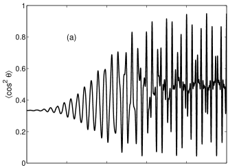
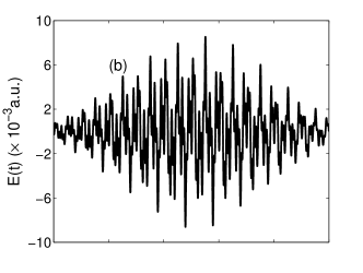
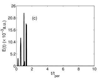
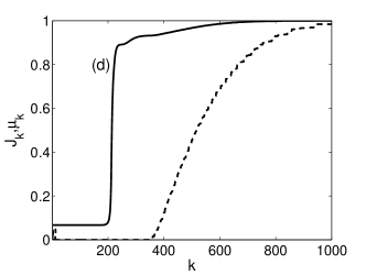
Figure 1: Plot as a function of the adimensional time $t/t_{per}$ of (a) the expectation value $\langle\cos^{2}\theta\rangle$ obtained from the algorithm with filtering, (b) the corresponding optimal filtered field and (c) the standard optimal field. (d) Plot as a function of the number of iterations $k$ of the adimensional cost $J_{k}$ (solid line) and of the parameter $\mu_{k}$ (dashed line) for the algorithm with filtering.

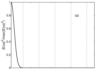
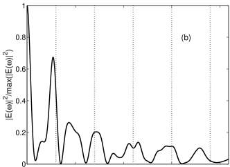
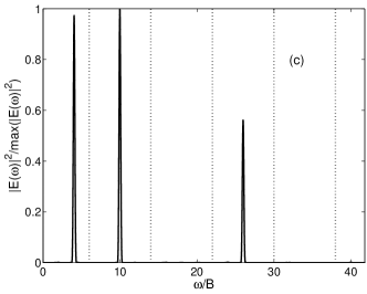
Figure 2: Normalized square modulus of the Fourier transform of the trial field (a), of the optimal field obtained by the standard algorithm (b) and of the optimal field obtained by the algorithm with filtering. The vertical dashed lines correspond to the rotational frequencies between two successive rotational levels.

3.2 Non-zero temperature

In this section, we test the efficiency of the algorithm at a non-zero temperature. The system is described by a density matrix with a dynamics governed by the von Neumann equation [37, 38]. The initial density matrix is the Boltzmann equilibrium density operator at temperature $T$. We use the target state $\rho_{opt}^{(j_{opt})}$ constructed in Ref. [50] for a linearly polarized electric field. This density matrix acts in the space $\mathcal{H}_{j_{opt}}$ with $j_{opt}=8$ which is chosen with respect to the temperature and the intensity of the field used. As before, we have used the algorithm of [27] with a cost functional similar to the one of Sec. 2. We have considered three temperatures $T=5,~{}7$ and 10 K and a shorter control field with a duration equal to one rotational period. The numerical parameters of the trial gaussian field are taken to be $37.5~{}\textrm{TW}/\textrm{cm}^{2}$ for the peak intensity and 1 ps for the duration (FWHM), except for $T=7~{}\textrm{K}$ where the duration is equal to 0.475 ps. 6000 iterations have been used for the first two temperatures and 8000 for the last one. The parameters of the algorithm are equal to $\lambda_{0}=1$ and $\eta=1$.

We have used a filtering which mimics experimental control techniques using liquid crystal pulse shapers [44]. Such pulse shapers work in the frequency domain by tailoring the spectral phase and amplitude of the electric field. This operation can be defined through a filter $\mathcal{F}$ which transforms over a given bandwidth the Fourier transform of the control field into a piecewise constant function in phase and in amplitude. The bandwidth is taken to be 7.28 THz which corresponds to two times the 5th rotational frequency. A larger bandwidth has given equivalent results. The filtered control field $\mathcal{F}(E(t))$ is finally obtained by an inverse Fourier transform. In the following computations, the number of pixels $N$ is equal to 64, 128 or 256 both in amplitude and in phase. The pixels that discretize the Fourier transform are taken equally spaced in the frequency interval defined by the bandwidth.

To determine the parameter $\mu_{k+1}$, we compute at each iteration $\Delta J_{k+1}(\mu)=J(E_{k+1,\mu})-J_{k}(\tilde{E}_{k})$ for 10 values of $\mu$ equally spaced in the interval $[0,1]$. Using these ten values, we construct a polynomial fit of $\Delta J_{k+1}(\mu)$. We define $\mu_{k+1}$ as the smallest value of $\mu$ such that $\Delta J_{k+1}(\mu_{k+1})=0.01\times\max_{\mu\in[0,1]}[\Delta J_{k+1}(\mu)]$. We have checked that these ten values are sufficient.

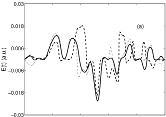
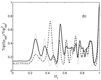
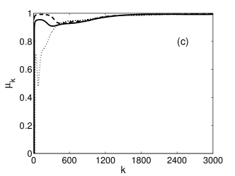
Figure 3: Plot as a function of the adimensional time $t/t_{f}$ of (a) the optimal electric field and (b) the projection onto the target state $\rho_{opt}$. (c) Plot as a function of the number of iteration $k$ of the parameter $\mu_{k}$. Solid, dashed and dotted lines correspond respectively to $T=10,~{}7$ and 5 K. The number of pixels is equal to 128.

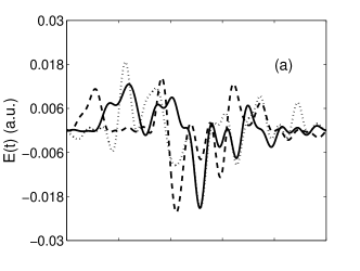
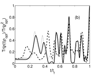
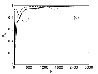
Figure 4: Same as Fig. 3 but for $T=5$ K and different numbers of pixels. Solid, dashed and dotted lines correspond respectively to $N=128,~{}64$ and 256 pixels.

The results obtained for the three temperatures are displayed in Fig. 3 with a fixed number of pixels equal to 128. Very efficient optimal fields have been constructed by the algorithm since a final projection of 99.2%, 97% and 93.5% has been obtained for respectively $T=5,~{}7$ and 10 K. As can be expected, the temperature has a negative effect on the alignment but the control remains robust with respect to the temperature. Note also the completely different structures of the three optimal fields leading to three different evolutions for the projection. This example shows that our algorithm can be used to construct realistic control fields both in temperature and in intensity. In Fig. 3c, one observes a similar evolution for the three parameters $\mu_{k}$ which are close to zero for the first hundred iterations and then quickly increase for $k\geq 100$. The increase of $\mu_{k}$ is more pronounced for higher temperatures which indicates that spectral constraints are more difficult to impose when the temperature increases.

Figures 4 illustrate the impact on the algorithm of the number of pixels. We have obtained a final projection of respectively 0.975, 0.989 and 0.992 for $N=64,~{}128$ and 256 pixels. In Fig. 4, we have represented the fields after a final filtering to get solutions that can be implemented experimentally. We then obtain 0.813, 0.892 and 0.926 for the three cases. The final result passes for $N=64$ from 0.975 to 0.813 which shows that the optimal solution does not satisfy very well the spectral constraints. One deduces that $N=64$ is not a sufficient number of pixels to construct the optimal field. This observation is also related to the rapid increase of $\mu_{k}$ in Fig. 4c for $N=64$. To summarize, this result indicates the minimum number of pixels that has to be used experimentally to control molecular alignment with an optimal control field.

4 Conclusion

We have proposed a new monotonically convergent algorithm to take into account spectral constraints. The procedure is built on the standard framework but at each iteration, the field is taken as a linear combination of the field given by the standard algorithm and its filtered version. The parameter of the linear combination is computed numerically to ensure the monotonic behavior of the algorithm.

This algorithm has the advantage of simplicity and general applicability whatever the filter chosen. We have presented two examples on molecular alignment using either bandpass filters or a discretization in the frequency domain mimicking pulse shaping techniques. This work leads to important insights into the different ways to achieve molecular alignment. Since there exists no unique optimal solution, we can select using spectral filters control fields taking into account experimental constraints. For instance, we have shown that the control can find a pathway using only three rotational frequencies to reach the aligned state. The spectral constraints have suppressed the other pathways simplifying therefore the structure of the control field.

This algorithm allows to test the choice of the filter with respect to the optimal field considered. Indeed, a value of $\mu_{k}$ close to 1 means that the filter is not well suited to the form of the electric field determined by the monotonic algorithm. This remark is particularly true for the first iterations of the algorithm since after the first iterations, the optimal field and the filtered field can be very close to each other. In the case of pulse shaping techniques, we can then determine from the algorithm the minimum number of pixels of the mask needed to reach a high alignment efficiency. This renders the use of optimal control theory more interesting from an experimental point of view by making a direct link with control experiments.

Appendix A Proof of the monotonic behavior of the algorithm

In this section, we show the monotonic behavior of the algorithm in the case of a nonlinear interaction with the control field. Let $\tilde{E}_{k}$ be the optimal field at step $k$ of the algorithm. We determine the field $E_{k+1}$ at step $k+1$ so that the variation $\Delta J=J(E_{k+1})-J(\tilde{E}_{k})\geq 0$ [27]. This variation is given by:

(9) $$\Delta J=|\langle\phi_{f}|\psi_{k+1}(t_{f})\rangle|^{2}-|\langle\phi_{f}|\psi_{k}(t_{f})\rangle|^{2}-\int_{0}^{t_{f}}\lambda[E_{k+1}(t)^{4}-\tilde{E}_{k}(t)^{4}]dt.$$

We introduce the function $P_{k+1}(t)=|\langle\chi_{k}(t)|\psi_{k+1}(t)\rangle|^{2}$. Differentiating it with respect to time produces

(10) $$\frac{d}{dt}P_{k+1}(t)=\alpha_{k,k+1}(\tilde{E}_{k}^{2}-E_{k+1}^{2})$$

where

$$\alpha_{k,k+1}=2\textrm{Im}[\langle\psi_{k+1}(t)|\chi_{k}(t)\rangle\langle\chi_{k}(t)|\frac{1}{4}(\cos^{2}\theta\Delta\alpha+\alpha_{\perp})|\psi_{k+1}(t)\rangle,$$

and a direct integration gives

(11) $$P_{k+1}(t_{f})=P_{k+1}(0)+\int_{0}^{t_{f}}\frac{dP_{k+1}}{dt}dt.$$

Using the relation $|\langle\phi_{f}|\psi_{k+1}(t_{f})\rangle|^{2}-|\langle\phi_{f}|\psi_{k}(t_{f})\rangle|^{2}=P_{k+1}(t_{f})-P_{k}(t_{f})$, straightforward computations lead to

(12) $$J(E_{k+1})-J(\tilde{E}_{k})=-\int_{0}^{t_{f}}[\lambda(t)(E_{k+1}^{4}-\tilde{E}_{k}^{4})-(\tilde{E}_{k}^{2}-E_{k+1}^{2})\alpha_{k,k+1}]dt.$$

The integrand $\mathcal{P}$ of $J(E_{k+1})-J(\tilde{E}_{k})$ can be written as follows:

$$\mathcal{P}=(E_{k+1}-\tilde{E}_{k})[-\lambda(E_{k+1}^{3}+E_{k+1}^{2}\tilde{E}_{k}+E_{k+1}\tilde{E}_{k}^{2}+\tilde{E}_{k}^{3})-\alpha_{k,k+1}(E_{k+1}+\tilde{E}_{k})].$$

We define the optimal electric field $E_{k+1}$ as the solution of:

$$E_{k+1}-\tilde{E}_{k}=\eta[-\lambda(E_{k+1}^{3}+E_{k+1}^{2}\tilde{E}_{k}+E_{k+1}\tilde{E}_{k}^{2}+\tilde{E}_{k}^{3})-\alpha_{k,k+1}(E_{k+1}+\tilde{E}_{k})],$$

where $\eta$ is a positive constant. It is straightforward to check that $J(E_{k+1})-J(\tilde{E}_{k})\geq 0$ for this choice of $E_{k+1}$.

References

- [1] W. Warren, H. Rabitz, and M. Dahleb, Science 259, 1581 (1993).
- [2] H. Rabitz, R. de Vivie-Riedle, M. Motzkus, and K. Kompa, Science 288, 824 (2000).
- [3] M. A. Nielsen and I. L. Chuang, Quantum Computation and Quantum Information (Cambridge University Press, Cambridge, 2000).
- [4] T. Baumert, T. Brixner, V. Seyfried, M. Strehle, and G. Gerber, Appl. Phys. B (1997).
- [5] C. Daniel, J. Full, L. Gonzàlez, C. Lupulescu, J. Manz, A. Merli, S. Vadja, and L. Woste, Science 299, 536 (2003).
- [6] R. S. Judson and H. Rabitz, Phys. Rev. Lett. 68, 1500 (1992).
- [7] A. Assion, T. Baumer, M. Bergt, T. Brixner, B. Kiefer, V. Seyfried, M. Strehle, and G. Gerber, Science 282, 919 (1998).
- [8] R. J. Levis, G. M. Menkir, and H. Rabitz, Science 292, 709 (2001).
- [9] M. Shapiro and P. Brumer, Principals of quantum control of molecular processes (Wiley, New York, 2003).
- [10] S. Rice and M. Zhao, Optimal control of molecular dynamics (Wiley, New York, 2000).
- [11] D. J. Tannor, Introduction to quantum mechanics: A time-dependent perspective (University science books, Sausalito, California, 2007).
- [12] V. Jurdjevic, Geometric Control Theory (Cambridge University Press, Cambridge, 1996).
- [13] B. Bonnard and M. Chyba, Singular trajectories and their role in control theory (Springer SMAI, VOL. 40, 2003).
- [14] U. Boscain, G. Charlot, J.-P. Gauthier, S. Guérin, and H. R. Jauslin, J. Math. Phys. 43, 2107 (2002).
- [15] D. Sugny, C. Kontz, and H. R. Jauslin, Phys. Rev. A 76, 023419 (2007a).
- [16] D. Sugny and C. Kontz, Phys. Rev. A 77, 063420 (2008).
- [17] R. Kosloff, S. Rice, P. Gaspard, S. Tersigni, and D. Tannor, Chem. Phys. 139, 201 (1989).
- [18] W. Zhu and H. Rabitz, J. Chem. Phys. 118, 6751 (2003).
- [19] W. Zhu and H. Rabitz, J. Chem. Phys. 110, 7142 (1999).
- [20] W. Zhu and H. Rabitz, J. Chem. Phys. 109, 385 (1998).
- [21] Y. Maday and G. Turinici, J. Chem. Phys. 118, 8191 (2003).
- [22] Y. Ohtsuki, W. Zhu, and H. Rabitz, J. Chem. Phys. 110, 9825 (1999).
- [23] Y. Ohtsuki, G. Turinici, and H. Rabitz, J. Chem. Phys. 120, 5509 (2004).
- [24] D. Sugny, M. Ndong, D. Lauvergnat, Y. Justum, and M. Desouter-Lecomte, J. Phot. Photob. A 190, 359 (2007b).
- [25] D. Sugny, C. Kontz, M. Ndong, Y. Justum, G. Dives, and M. Desouter-Lecomte, Phys. Rev. A 74, 043419 (2006a).
- [26] M. Ndong, L. Bomble, D. Sugny, Y. Justum, and M. Desouter-Lecomte, Phys. Rev. A 76, 043424 (2007).
- [27] M. Lapert, R. Tehini, G. Turinici, and D. Sugny, Phys. Rev. A 78, 023408 (2008).
- [28] Y. Ohtsuki and K. Nakagami, Phys. Rev. A 77, 033414 (2008).
- [29] K. Nakagami, Y. Mizumoto, and Y. Ohtsuki, J. Chem. Phys. 129, 194103 (2008).
- [30] R. Tehini and D. Sugny, Phys. Rev. A 77, 023407 (2008).
- [31] C. Gollub, M. Kowalewski, and R. de Vivie-Riedle, Phys. Rev. Lett. 101, 073002 (2008).
- [32] J. Werschnik and E. K. U. Gross, J. Opt. B: Quantum Semi-class. Opt. 7, S (2005).
- [33] M. Artamonov, T.-S. Ho, and H. Rabitz, Chem. Phys. 305, 213 (2004).
- [34] T. Hornung, M. Motzkus, and R. de Vivie-Riedle, J. Chem. Phys. 115, 3105 (2001).
- [35] P. Gross, D. Neuhauser, and H. Rabitz, J. Chem. Phys. 96, 2834 (1992).
- [36] B. Friedrich and D. Herschbach, Phys. Rev. Lett. 74, 4623 (1995).
- [37] T. Seideman and E. Hamilton, Adv. At. Mol. Opt. Phys. 52, 289 (2006).
- [38] H. Stapelfeldt and T. Seideman, Rev. Mod. Phys. 75, 543 (2003).
- [39] C. Horn, M. Wollenhaupt, M. Krug, T. Baumert, R. de Nalda, and L. Banares, Phys. Rev. A 73, 031401 (2006).
- [40] M. D. Poulsen, T. Ejdrup, H. Stapelfeldt, E. Hamilton, and T. Seideman, Phys. Rev. A 73, 033405 (2006).
- [41] C. Z. Bisgaard, M. D. Poulsen, E. Péronne, S. S. Viftrup, and H. Stapelfeldt, Phys. Rev. Lett. 92, 173004 (2004).
- [42] C. Z. Bisgaard, S. S. Viftrup, and H. Stapelfeldt, Phys. Rev. A 73, 053410 (2006).
- [43] O. M. Shir, V. Beltrani, T. Back, H. Rabitz, and M. J. J. Vrakking, J. Phys. B 41, 074021 (2008).
- [44] E. Hertz, A. Rouzée, S. Guérin, B. Lavorel, and O. Faucher, Phys. Rev. A 75, 031403(R) (2007).
- [45] A. Rouzée, E. Hertz, B. Lavorel, and O. Faucher, J. Phys. B 41, 074002 (2008).
- [46] J. Salomon, C. M. Dion, and G. Turinici, J. Chem. Phys. 123, 144310 (2005).
- [47] A. Pelzer, S. Ramakrishna, and T. Seideman, J. Chem. Phys. 126, 034503 (2007).
- [48] H. Sekino and R. J. Bartlett, J. Chem. Phys. 98, 3022 (1993).
- [49] D. Sugny, A. Keller, O. Atabek, D. Daems, C. M. Dion, S. Guérin, and H. R. Jauslin, Phys. Rev. A 71, 063402 (2005a).
- [50] D. Sugny, A. Keller, O. Atabek, D. Daems, C. M. Dion, S. Guérin, and H. R. Jauslin, Phys. Rev. A 72, 032704 (2005b).
- [51] D. Sugny, C. Kontz, and H. R. Jauslin, Phys. Rev. A 74, 053411 (2006b).
- [52] A. Pelzer, S. Ramakrishna, and T. Seideman, J. Chem. Phys. 129, 134301 (2008).
- [53] K. Sundermann and R. de Vivie-Riedle, J. Chem. Phys. 110, 1896 (1999).