Pixel-lensing as a way to detect extrasolar planets in M31

Abstract

We study the possibility to detect extrasolar planets in M31 through pixel-lensing observations. Using a Monte Carlo approach, we select the physical parameters of the binary lens system, a star hosting a planet, and we calculate the pixel-lensing light curve taking into account the finite source effects. Indeed, their inclusion is crucial since the sources in M31 microlensing events are mainly giant stars. Light curves with detectable planetary features are selected by looking for significant deviations from the corresponding Paczyński shapes. We find that the time scale of planetary deviations in light curves increase (up to 3-4 days) as the source size increases. This means that only few exposures per day, depending also on the required accuracy, may be sufficient to reveal in the light curve a planetary companion. Although the mean planet mass for the selected events is about $2~{}M_{\rm{Jupiter}}$, even small mass planets ($M_{\rm P}<20~{}M_{\oplus}$) can cause significant deviations, at least in the observations with large telescopes. However, even in the former case, the probability to find detectable planetary features in pixel-lensing light curves is at most a few percent of the detectable events, and therefore many events have to be collected in order to detect an extrasolar planet in M31. Our analysis also supports the claim that the anomaly found in the candidate event PA-99-N2 towards M31 can be explained by a companion object orbiting the lens star.

1 Introduction

In the last years, it has become clear that gravitational microlensing, initially developed to search for MACHOs in our Galactic halo and near the Galactic disk (Paczyński, 1986; Alcock et al., 1993; Paczyński, 1996; Roulet & Mollerach, 1997, 2002; Zakharov & Sazhin, 1998) can be used to infer the presence of extrasolar planets orbiting around lens stars (see the review by Perryman 2000; Perryman et al. 2005; Bennett 2009).

As shown by Mao & Paczyński (1991) the planet presence effect on the light curve in a microlensing event towards the Galactic bulge is generally a short duration perturbation to the standard microlensing curve. These deviations last from a few hours to some days (depending on the planet mass) and can occur relatively frequently, even for rather small mass planets. Indeed, the microlensing technique is sensitive to planets in a rather large range of masses, from Jupiter-like planets down to Earth-like ones (Bennett & Rhie, 1996).

Gould & Loeb (1992) pointed out that there is a significant probability to detect planets around stars in the Galactic disk that act as microlenses by magnifying the light of observed stars in the Galactic bulge. Until now, the detection of eight extrasolar planets has been reported by using the microlensing technique (Bond et al., 2004; Udalski et al., 2005; Beaulieu et al., 2006; Gould et al., 2006; Gaudi et al., 2008; Bennett, 2009). We remind that the masses of three of them ($\simeq$ 3, 5 and 13 $M_{\oplus}$) are at the lower bound of the detected planetary mass range. Indeed, more than 300 extrasolar planets discovered until now by radial velocity, transit and direct imaging methods are biased towards large mass (Jupiter-like) planets (Ida & Lin, 2004). However, radial velocity searches by ground based experiments have now provided extrasolar planets with $M_{\rm min}=2~{}M_{\oplus}$ (Mayor et al., 2009), whereas space based observations are expected to detect many Earth-mass planets (with Kepler satellite ) and many Earth-size planets (with COROT spececraft ).

A further advantage of the microlensing is that it works better for large distance of the source star, since the optical depth increases by increasing the distance, as one can already see from the Einstein (1936) approach. This gives the opportunity to detect planetary systems at distances much larger with respect to those accessible by the other tecniques and even in other galaxies such as M31 (see, e.g., Covone et al. 2000; Baltz & Gondolo 2001). In this case, however, the source stars are not resolved by ground based telescopes - a situation referred to as “pixel-lensing” (Crotts, 1992; Baillon et al., 1993; Gould, 1996) - and only bright sources (i.e. giant stars with large radii), sufficiently magnified, can give rise to detectable microlensing events (Ansari et al., 1997). This implies that finite size effects, leading to smaller planetary deviations in pixel-lensing light-curves with respect to microlensing towards the galactic bulge, cannot be neglected (see, e.g., Riffeser, Seitz & Bender 2008). Usually, highly magnified events arise when the source and lens stars align very closely. In this case there is the largest chance of observing the perturbations in the light curves induced by planets (Griest & Safizadeh, 1998). This is particularly true for large mass planets, for which the planetary signals are not strongly suppressed by finite size effects, whereas for low mass planets, the planetary signals may remain detectable during other phases of the event (Bennett, 2009).

Until now, only about a dozen microlensing events have been observed towards M31 by the POINT-AGAPE (Calchi Novati et al., 2005) and MEGA collaborations (de Jong et al., 2006). Only in one case a deviation from the standard Paczyński shape has been observed and attributed to a secondary component orbiting the lens star (An et al., 2004). However, new observational campaigns towards M31 have been undertaken (Kerins et al., 2006; Calchi Novati et al., 2007, 2009) and hopefully a few planets might be detected in the future, providing a better statistics on the masses and orbital radii of extrasolar planets. It is in fact expected, and supported by observations and numerical simulations, that almost any star has at least a planet orbiting around it (see, e.g., Lineweaver & Grether 2003). In other words, as also suggested by Baltz & Gondolo (2001), the rate of single lens events towards M31 may suffer of a strong contamination of binary lensing events, most of which are expected to be due to extrasolar planets.

Therefore, it is important to address the question of how to extract information about planetary lensing events, occurring in M31, from the observed microlensing light curves. Since planetary perturbations last from hours to a few days, a monitoring program with suitable sampling must be realised, in order to avoid missing these perturbations. The feasibility of such research program has been already explored by Chung et al. (2006) and Kim et al. (2007). They have considered the possibility to detect planets in M31 bulge by using the observations taken from the Angstrom collaboration (Kerins et al., 2006) with a global network of 2 m class telescopes and a monitoring frequency of about five observations per day. The analysis for planet detection, however, has been performed by using a fixed configuration of the underlying Paczyński light curve.

In the present work, instead, by using a Monte Carlo (MC) approach (De Paolis et al., 2005; Ingrosso et al., 2006, 2007) we explore the possibility of detecting extrasolar planets in pixel-lensing observations towards M31, by considering the multi-dimensional space of parameters for both lensing and planetary systems. Taking into account the finite source effects and the limb darkening and using the residual method we can select the simulated light curves that show significant deviations with respect to a Paczyński like light curve, modified by finite source effects. The advantage of the Monte Carlo approach is that of allowing us a complete characterization of the sample of microlensing events for which the planetary deviations are more likely to be detected.

The paper is structured as follows. In Section 2, we give the basics of binary-lensing events. In Section 3 we discuss our MC simulations for planetary detection in M31. In section 4 we present our main results and in Section 5 we address the conclusions.

2 Binary-lensing events

2.1 Generalities

If a source star is gravitationally lensed by a binary lens, the equation of lens mapping from the lens plane to the source plane can be expressed in complex notation (Witt, 1990; Witt & Mao, 1995)

$$\xi(\zeta,\eta)=z-\sum_{j=1}^{2}\frac{m_{j}/M}{\bar{z}-\bar{z}_{L,j}}~{},$$ (1)

where $\xi=\zeta+i\eta$ and $z=x+iy$ are the source and the image positions, $\bar{z}$ is the complex conjugate of $z$, $m_{1}$, $m_{2}$, $z_{L,1}$ and $z_{L,2}$ are the the masses and the positions of the two lenses, respectively. Here and in the following, all the lengths (angular separations) are normalized to the radius $R_{\mathrm{E}}$ (angle $\theta_{\rm E}$) of the Einstein ring which are related to the physical parameter of the lens by

$$R_{\mathrm{E}}=\left[\left(\frac{4GM}{c^{2}}\right)\frac{D_{\rm L}(D_{\rm S}-D_{\rm L})}{D_{\rm S}}\right]^{1/2}~{}~{}~{}~{}~{}{\rm and}~{}~{}~{}\theta_{\rm E}=\frac{R_{\rm E}}{D_{\rm L}}~{},$$ (2)

where $M=m_{1}+m_{2}$ is the total mass of the binary system, $D_{\rm L}$ and $D_{\rm S}$ are the distances to the lens and to the source, respectively. Under the condition $m_{1}>m_{2}$, we define the mass ratio parameter $q=m_{2}/m_{1}$. In addition, we assume that the two masses of the binary system are located on the real axis, with the centre of mass in the origin. Let us denote with $d$ the angular separation between the two objects in units of $\theta_{\rm E}$.

To determine the image position and magnification, one has to take the complex conjugate of equation (1) and substitute the expression for $\bar{z}$ back in it, obtaining a fifth-order polynomial in $z$, i. e. $p(z)=\sum_{i=1}^{5}c_{i}z^{i}=0$ (with coefficients $c_{i}$ depending on $M$, $d$, and $q$), whose solutions give the image positions. Due to lensing, the source star image splits into several fragments up to a total number $N_{I}$. Since the lensing process conserves the source brightness and thus the magnification of each image, the total magnification corresponds to the sum over all images (Witt & Mao, 1995), i. e.

$$A_{\rm P}=\sum_{i}^{N_{I}}\left(\frac{p(z_{i})}{\det J}\right)~{},$$ (3)

where the determinant of the Jacobian is

$$\det J=1-\frac{\partial\xi}{\partial\overline{z}}\frac{\overline{\partial\xi}}{\partial\overline{z}}~{}.$$ (4)

A planetary lens system is characterized by the condition that the planet mass $M_{\rm P}=m_{2}$ is much smaller with respect to the host star mass $M_{\rm L}=m_{1}$. In this case, the planet only induces a perturbation on the underlying Paczyński curve of the primary lens. Planet perturbations occur when the source star crosses and/or passes near caustics, which are the set of source positions on the $(\zeta,\eta)$ plane at which the magnification is infinite (i.e. those corresponding to $\det J=0$) in the idealized case of a point source. Clearly, for realistic sources of finite size the magnitude gets still quite large, but finite (Witt & Mao, 1994). Caustics form a single or multiple sets of closed and concave curves (fold caustics) which meet in cusp points (Schneider, Ehlers & Falco, 1992; Schneider & Weiss, 1992; Zakharov & Sazhin, 1995). The location of the planet perturbations depends on the position of the caustics and the source trajectory.

There have been several attempts to determine caustic positions and shapes by using analytic methods and treating the planet induced deviations as a perturbation (Gaudi & Gould, 1997; Dominik, 1999; Bozza, 1999). For the planetary case, there exists two sets of caustics: “central” and “planetary”. The single, central caustic is located on the star-to-planet axis, close to the host star. For a wide range of parameters the caustic has a diamond shape and can be described by parametric equations (as it was shown by Zakharov & Sazhin 1997a, b, central astroid caustics arise if the Chang & Refsdal 1984a, b model is used). Planetary caustics are located away from the host star, at distance $\simeq(d^{2}-1)/d$ from the primary lens position. There is one planetary caustic (with a diamond shape) on the star-to-planet axis, on the planet side, when $d>1$ and two sets of caustics, off the axis, (with triangular shape) on the star side when $d<1$. The dimensions of both central and planetary caustics increase by increasing the mass ratio $q$ (Zakharov & Sazhin, 1998; Bozza, 1999; Chung et al., 2005; Han & Gaudi, 2008). Moreover, for a given $q$ value, the caustic sizes are maximized when the planet is inside the so called “lensing zone”, which is defined (with some arbitrariness) as the range of star-to-planet separation $0.6\mathop{\vtop{\halign{#\cr$\hfil\displaystyle{<}\hfil$\crcr\kern 1.0pt\nointerlineskip\cr\hbox{$\hfil\sim\hfil$}\crcr\kern 1.0pt\cr}}}d\mathop{\vtop{\halign{#\cr$\hfil\displaystyle{<}\hfil$\crcr\kern 1.0pt\nointerlineskip\cr\hbox{$\hfil\sim\hfil$}\crcr\kern 1.0pt\cr}}}1.6$ (Gould & Loeb, 1992; Griest & Safizadeh, 1998). The time duration scale of the perturbations induced by a planet and the probability of their detection are proportional to the caustic size, at least when this region is large enough so that the planetary signals are not suppressed by the finite source effects (Mao & Paczyński, 1991; Bolatto & Falco, 1994; Gould & Loeb, 1992).

2.2 Finite source approximation

Since in pixel-lensing towards M31 the bulk of the source stars are red giants (see Section 3), one has to take into account the source finiteness. This leads to smaller planetary deviations in pixel-lensing light curves with respect to microlensing towards the galactic bulge, for which the point-like source approximation is acceptable. For finite source effects with limb darkening the magnification has to be numerically evaluated (see, e.g., Schneider, Ehlers & Falco 1992; Bogdanov & Cherepashchuk 1995a; Dominik 2005 and references therein)

$$\langle A_{\rm P}(t)\rangle=\frac{\int_{0}^{2\pi}d\theta\int_{0}^{\rho}A_{\rm P}(\tilde{\theta},\tilde{\rho};t)I(\tilde{\rho})\tilde{\rho}d\tilde{\rho}}{2\pi\int_{0}^{\rho}I(\tilde{\rho})\tilde{\rho}d\tilde{\rho}}~{},$$ (5)

where $\rho={\theta_{\rm S}}/{\theta_{\rm E}}$ is the normalized angular size of the source ($\theta_{\rm S}=R_{\rm S}/D_{\rm S}$, $R_{\rm S}$ being the source radius), and $I(\tilde{\rho})$ is the intensity profile of the source including limb darkening, for which we use the Claret (2000) approximation

$$I(\tilde{\rho})=1-a_{1}(1-\mu^{1/2})-a_{2}(1-\mu)-a_{3}(1-\mu^{3/2})-a_{4}(1-\mu^{2})~{},$$ (6)

with $\mu=\tilde{\rho}/\rho$ and the coefficients in the $R$-band are $a_{1}=0.8282$, $a_{2}=-0.9866$, $a_{3}=1.6801$ and $a_{4}=-0.6604$ (for red giant stars).

Moreover, since during caustic crossing the magnification could have strong changes and (at least for small mass planets and/or realistic source sizes) typical time scale for crossing could be comparable with the exposure time $t_{\rm exp}$ (needed to have a reasonable signal-to-noise level) we take the average magnification of equation (5) in the interval $(t-t_{\rm exp}/2,t+t_{\rm exp}/2)$.

Finite size source effects can be relevant for two reasons. First, the relationship between the dimensionless radius $\rho$ and the impact parameter $u_{0}$ determines if the finite size effects are important or not for the main microlensing light curve. This occurs in the events with $\rho/u_{0}>1$ or $\rho/u_{0}<1$, respectively. Second, finite size effects may be important for the planetary deviations even if they are not relevant for microlensing without planets. Indeed, $\rho$ is to be compared not only with $u_{0}$, but also with the caustic size $\Delta$. In particular, whenever $\rho/u_{0}>1$, it results that $\rho$ is typically much larger than $\Delta$ (at least for small enough mass planets). In this case, smoothed planetary deviations are produced in the light curves, since the planetary magnification has to be averaged on the source area. In a similar way, depending on the lens system geometry and proper motion, whenever the ratio $\rho/u_{0}<1$, stronger and temporally localized planetary deviations are produced in the light curves, since the caustic region results to be a non negligible fraction of the source area. Within the following analysis for the detection of planetary deviations we are going to identify two classes (I and II) of events, depending on the ratio $\rho/u_{0}>1$ and $\rho/u_{0}<1$, respectively .

3 Monte Carlo simulation

3.1 Light curve generation

In the present analysis we assume that the lens is a binary system constituted by a star and a planet companion . Our aim is to evaluate the probability to detect the presence of planets in M31 through Earth-based pixel-lensing observations with telescopes of different diameters. These telescopes could be initiated to observe towards a microlensing event candidate, so making a high cadence observations of an ongoing microlensing event. As reference values, we adopt a CCD pixel field of view of 0.2 arcsec, a typical seeing value of 1 arcsec and an average background luminosity at telescope site of $\simeq 21$ mag arcsec^-2 in $R$-band. To have a good S/N ratio we consider in the MC analysis exposure times $t_{\rm exp}$ of 30 minutes. Moreover, we assume a regular sampling neglecting any loss of coverage due to bad weather conditions.

In order to take into account the spatial variation of the background level we select four directions (named ${\bf A,~{}B,~{}C,~{}D}$) at increasing distances from the M31 centre. Assuming a coordinate system with origin in the M31 centre and axes along the north-south and east-west directions, the coordinates of the selected directions are the following: $\bf A$ (–6,0) arcmin, $\bf B$ (–9,0) arcmin, $\bf C$ (–12,0) arcmin, $\bf D$ (–21,–6) arcmin. In the direction $\bf A$ the microlensing is primarily due to self-lensing events by stars in the M31 bulge and disk, whereas towards the external directions the contribution to microlensing due to lenses belonging to the M31 halo becomes larger. Our investigation of the $\bf D$ direction is motivated by the detection of the anomaly in the pixel-lensing event PA-99-N2 (An et al., 2004).

As for the generation of the trial microlensing light curves we closely follow the approach outlined by Kerins et al. (2001). The adopted M31 astrophysical model was described by Ingrosso et al. (2006). Once the event location has been selected, for any lens and source population lying along the line of sight, we use a MC approach to select the physical parameters of the systems: source magnitude, primary lens mass, source and lens distances, effective transverse velocity of source and lens, impact parameter of the lens.

The luminosity of star sources, mainly red giants in the interval of absolute magnitude $(-4,~{}2.4)$, and the corresponding radii are drawn from a sample of stars generated by a synthetic color-magnitude diagram computation algorithm described by Aparicio & Gallart (2004) based on the stellar evolution library (Bertelli et al., 1994) and the bolometric correction database (Girardi et al., 2002).

As next, we have to select the mass $M_{\rm P}$ and the (projected) orbital distance $d_{\rm P}$ of the extrasolar planet. Most of the hundreds of extrasolar planets discovered up to now (see the web site http://exoplanet.eu) have typically very large masses and orbit at small distances around their parent stars (Udry & Santos, 2007). This appears to be a result of observational biases (Ida & Lin, 2004) since most of the planets have been detected by radial velocity and transit techniques that are most sensitive to massive and close planets. Direct imaging and microlensing techniques contribute only a minor fraction of the detected events. Indeed, available theoretical and numerical analysis show that most extrasolar planets are expected to have relatively smaller masses. Furthermore, the (projected) orbital distance from their hosting stars is expected in the range $\simeq 0.04-100$ AU (see, e.g., Tabachnik & Tremaine 2002; Ida & Lin 2004). In the present paper we assume that the distribution of $M_{\rm P}$ and orbital period $P$, for $M_{\rm P}<10M_{\rm{Jupiter}}$, is given by the simple analytical expression (Tabachnik & Tremaine, 2002)

$$dn(M_{\rm P},P)=C~{}M_{\rm P}^{-\alpha}~{}P^{-\beta}~{}\left(\frac{dM_{\rm P}}{M_{\rm P}}\right)~{}\left(\frac{dP}{P}\right)~{}~{},$$ (7)

with $\alpha=0.11$ and $\beta=-0.27$. This relation is obtained by investigating the distribution of masses and orbital periods of 72 extrasolar planets, taking into account the selection effects caused by the limited velocity precision and duration of existing surveys. We note that in the analysis leading to the above distribution, it was assumed that the stars in the survey are of solar type, and therefore any dependence (as implied by recent extrasolar planet observations) of the planet mass on the parent star mass and metallicity has been neglected. Taking that into account, one would certainly replace equation (7) with a different one, and therefore the results presented in Section 4 for the detectable planet rate would change. For example, a steeper planet mass distribution (as that found for all Doppler-detected planets by Johnson (2009) with $\alpha=0.4$) implies a smaller (about a quarter) overall planet detection rate, as a consequence of the decrease of the mean planet mass. More importantly, a dependence of the planet mass distribution on the parent star mass would introduce a dependence of the planet detection rate on the lens population (bulge or disk stars) that could be recognized, provided a sufficient event statistics towards different lines of sight would be available. In equation (7), the upper limit of the planetary mass is set at $M_{\rm P}=10~{}M_{\rm{Jupiter}}$. This roughly corresponds to the usually assumed lower mass limit for brown dwarfs. Indeed, in the range $10-20~{}M_{\rm{Jupiter}}$ the two populations overlap. Moreover, in the simulation we select a lower planetary mass limit of $0.1~{}M_{\oplus}$. Once the masses of the binary components and the planet period have been selected, the binary separation $d_{\rm P}$ is obtained by assuming a circular motion of the planet.

As a parameter in our MC analysis we introduce the number $N_{\rm im}$ of images per day. We take $N_{\rm im}$ in the range 2 – 12 day^-1, the latter value corresponding to a sampling time of two hours. For all selected values of $N_{\rm im}$, the corresponding binary light curve at any time is given by

$$S_{\rm P}(t)=f_{\rm bl}+f_{0}\left(\langle A_{\rm P}(t)\rangle-1\right)~{},$$ (8)

where $f_{\rm bl}$ is the background signal from the galaxy and the sky, $f_{0}$ is the unamplified source star flux and $\langle A_{\rm P}(t)\rangle$ the time varying magnification, that takes into account both the source finiteness and the motion of the lens-source-observer system during the exposure time $t_{\rm exp}$. To mimic superpixel photometry (Ansari et al., 1997) used in a real observational campaign we evaluate the star and the background flux within a $n$-pixel square “superpixel”, whose size $n$ is determined to cover most of the average seeing disk. We recall that we consider the pixel-lensing regime where the noise is dominated by the (line of sight dependent) background noise (Kerins et al., 2001). Accordingly, we add to $S_{\rm P}(t)$ a Gaussian noise.

3.2 Microlensing event selection

As a first step, within the MC simulation, we have to test whether the flux variation due to the microlensing event is significant with respect to the background noise $\sigma(x,y)$, where $(x,y)$ identifies the line-of-sight. To asses the detection of a flux variation we evaluate its statistical significance testing whenever and to what extent at least three consecutive points exceed the baseline level by 3$\sigma$, following the analysis described by Calchi Novati et al. (2002). We remark that the condition on the variation significance is the only one used at this stage. In the following we refer to events that show a significant flux variations as to “detectable” events.

3.3 Planet detection

The expected signature of an extrasolar planet orbiting the lens star is the presence of perturbations with respect to the corresponding smooth Paczyński light curve. Therefore, we look for a selection criterion based on the analysis of the significance of such deviations. To this purpose, given the wide range of the microlensing parameters and the corresponding planetary deviations, we consider two indicators for which we select (by the direct survey of many light curves) threshold values. They are the mean deviation (in units of $\sigma$) of the planetary light curve from that of a single lens event, and the maximum value of the time dependent relative planetary magnification (in units of the expected Paczyński value).

At first, we fit the light curve in equation (8) with a Paczyński-like law modified to take into account finite source effects and determine the best fit parameters. The latter are the baseline flux $f_{\rm bl}^{0}$, the maximum magnification time $t_{0}^{0}$, the unamplified star flux $f_{0}^{0}$, the Einstein time $t_{\mathrm{E}}^{0}$, the dimensionless impact parameter $u_{0}^{0}$ and the dimensionless, projected star radius $\rho^{0}$. Accordingly, the time dependent flux $S^{0}(t)$ due to a single lens event is given by

$$S^{0}(t)=f_{\rm bl}^{0}+f_{0}^{0}\left(\langle A^{0}(t)\rangle-1\right)~{},$$ (9)

where the magnification (Einstein, 1936; Paczyński, 1986)

$$A^{0}(t)=\frac{u^{0}(t)^{2}+2}{u^{0}(t)\sqrt{u^{0}(t)^{2}+4}}$$ (10)

is given in terms of the time varying (normalized) lens angular distance to the source $u^{0}(t)$

$$u^{0}(t)=\sqrt{[u^{0}_{0}]^{2}+[(t-t^{0}_{0})/t^{0}_{\rm E}]^{2}}~{},$$ (11)

and $\langle A^{0}(t)\rangle$ is the analogous of equation (5), in this case evaluated by using the analytical approximation given by Witt & Mao (1994). Then, we can evaluate the time dependent variable

$$\chi^{2}(t)=(S_{\rm P}(t)-S^{0}(t))^{2}/\sigma^{2}(t)~{},$$ (12)

and the residual to the single lens fit

$$\chi_{\rm r}^{2}(t)=\left(1-\chi^{2}(t)\right)^{2}~{},$$ (13)

where $S_{\rm P}(t)$ is the light curve including the planet perturbations, $S^{0}(t)$ the Paczyński fit as above and $\sigma(t)$ is evaluated according to Kerins et al. (2001). Therefore, we can consider large values of $\chi_{\rm r}^{2}(t)$ as a significant indicator of the presence of detectable planetary deviations in the light curves. Actually, we use the sum of the residuals along the whole light curve, namely $\chi_{\rm r}^{2}=\sum_{i}\chi_{\rm r}^{2}(t_{i})/N_{\rm tot}$, as a first quantitative measure of the statistical significance of the planetary signals in the ongoing microlensing event. Here $t_{\rm i}=t_{0}+[(t_{\rm f}-t_{0})/N_{\rm tot}]~{}i$, where $t_{0}$ ($t_{\rm f}$) is the initial (final) instant and $N_{\rm tot}$ the total number of points. By the direct survey of many light curves we select a threshold value $\chi_{\rm r{~{}\rm th}}=4$. We further require a minimal number of points $N_{\rm good}$, even not consecutive, which deviate significantly (over $3\sigma$) from the Paczyński best fit. We adopt the criterion (i) $\chi_{\rm r}>\chi_{\rm r{~{}\rm th}}=4$ and $N_{\rm good}>N_{\rm good~{}th}=3$. In other words, the latter condition means that if we have significant deviations at only one or two points, we cannot conclude that they are caused by a planet orbiting the primary lens.

Figure 1: Normalized (to unity) distributions of $t_{1/2}$ (the duration of a microlensing event without planet). Top panel: detectable events. Bottom panel: selected events ($\chi_{\rm r}>4$, $N_{\rm good}>3$ and $\langle\epsilon\rangle_{\rm max}>0.1$) for I class ($\rho/u_{0}>1$, solid line) and II class ($\rho/u_{0}<1$, dashed line) events. In Figs. 1 – 11 we take $D=8$ m telescope parameters and $N_{\rm im}=12$ day^-1.

Figure 2: Normalized (to unity) distributions of $R_{max}$ (the magnitude corresponding to the flux variation at the maximal Paczyński magnification). Top panel: detectable events. Bottom panel: selected events for I class ($\rho/u_{0}>1$, solid line) and II class ($\rho/u_{0}<1$, dashed line) events. Here we take $D=8$ m telescope parameters.

The light curves fulfilling the above condition (i) may show only an overall distortion with respect to the underlying Paczyńsky shape. This is characteristics, in particular, for events with large source radii and small planetary masses. Our second criterion is therefore meant to look for and quantify the single more significant planetary perturbations. To this purpose we consider the time dependent, average (with respect to the source area $\Sigma$) relative planetary magnification

$$\langle\epsilon(t)\rangle=\left(\frac{\int_{\Sigma}d^{2}\vec{x}~{}[|A_{\rm P}(\vec{x},t)-A^{0}(\vec{x},t)|/A^{0}(\vec{x},t)]}{\int_{\Sigma}d^{2}\vec{x}}\right)~{}.$$ (14)

This quantity is sensibly different from zero only when, depending on the source and lens parameters and relative motion, there is (at a given time) a substantial overlapping between the source area and the caustic (central and/or planetary) region. So, to select light curves with detectable planetary features, besides condition (i), we further require that (ii) there exist at least one point on the light curve with $\langle\epsilon\rangle_{\rm max}$ larger than $\langle\epsilon\rangle_{\rm th}=0.1$. By using both conditions the number of selected events get reduced of about 50% with respect to the events selected by using only the condition (i). The condition (i) is particularly efficient to select light curves with a large number of points deviating from the Paczyński fit, the condition (ii) ensures the presence on the light curve of at least one clear planetary feature. Note that in this analysis we do not attempt to further characterize the planet deviations as due to intersection of central and/or planetary caustics.

4 Results

Table 1: Parameters of events shown in Figs. 3 - 6. We also give some microlensing parameters and in the last three columns the sum of residuals $\chi_{\rm r}$ along the whole light curve, the sum of residuals $\chi_{\rm r~{}max}$ and the maximum value of the relative planetary magnification $\langle\epsilon\rangle_{\rm max}$ during the time interval corresponding to the strongest planetary feature.

	$\rho/u_{0}$	$u_{0}$	$d_{\rm P}/R_{\rm E}$	$M_{\rm P}$	$\theta$	$R_{\rm E}$	$t_{\rm E}$	$R_{\rm max}$	$t_{1/2}$	$\chi_{\rm r}$	$\chi_{\rm r~{}max}$	$\langle\epsilon\rangle_{\rm max}$
				($M_{\rm{Jupiter}})$	(deg)	(AU)	(day)	(mag)	(day)
#1	2.89	$9.47\times 10^{-3}$	0.90	4.74	341.8	2.2	16.1	20.2	0.5	194	730	0.64
#2	1.18	$2.63\times 10^{-2}$	0.68	0.82	104.8	2.8	52.1	21.1	4.0	43	980	0.25
#3	0.12	$3.56\times 10^{-1}$	2.25	0.22	190.3	2.3	18.7	23.5	16.5	13	79	0.57
#4	0.08	$1.62\times 10^{-1}$	1.32	3.97	336.0	3.9	28.4	23.8	13.3	37	153	1.13

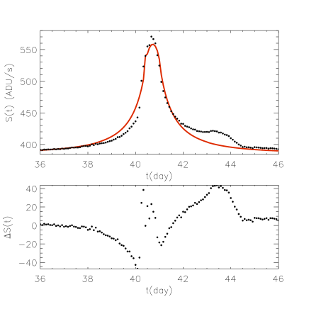
Figure 3: Event of the I class #1 (see Table 1). The upper panel shows the simulated light curve (black dots) and the corresponding best fit model (continuous line), that is a Paczyński light curve modified for finite source effects. The bottom panel gives the difference.

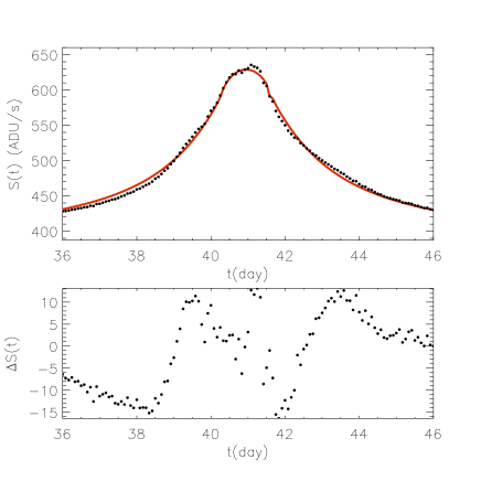
Figure 4: The same as in Fig. 3 for the I class event #2 (see Table 1).

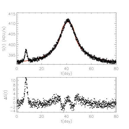
Figure 5: The same as in Fig. 3 for the II class event #3 (see Table 1). We note that the fit follows the simulated data except for a small time interval ($5<t<10$ day).

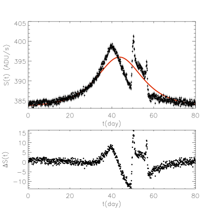
Figure 6: The same as in Fig. 3 for the II class event #4 (see Table 1).

In the following analysis we consider four different telescope diameters $D=1.5,~{}2.5,~{}4$ and 8 m (corresponding to zero-point in the $R$-band of $23.1~{},24.3,~{}25.3$ and 26.8 mag, respectively), $t_{\rm exp}=30$ min for all cases and we take $N_{\rm im}=12$ day^-1, corresponding to a regular sampling time of two hours. The effect of taking larger telescopes is that of increasing the number of faint, detectable events. Moreover, we consider only self-lensing events towards the four considered lines of sight (see Section 3.1), leaving out the eventual MACHO component in the galactic halos and assume the presence of a planet orbiting around each star in the M31 bulge and disk.

An advantage of the Monte Carlo approach to the binary microlensing analysis is that we can characterize the events with planetary detections. We remind that these events have been selected, from the whole sample of detectable events, by requiring $\chi_{\rm r}>4$, $N_{\rm good}>3$ and $\langle\epsilon\rangle_{\rm max}>0.1$.

In the Figs. 1 and 2 (for $D=8$ m) we give the distributions of $t_{1/2}$ and $R_{\rm max}$ for detectable (top panels) and selected events (bottom panels) . As usual (see, e.g., Kerins et al. 2001), $t_{1/2}$ is the full-width half-maximum microlensing event duration and $R_{\rm max}$ the magnitude in the $R$-band corresponding to the flux variation at the maximal Paczyński magnification. Comparing the corresponding distributions, we see that events with short time duration and large flux variation (therefore with smaller impact parameter) have a larger probability to show planetary deviations. This result is due to the fact that the crossing of the central caustic (close to the primary lens star) by the source trajectory is more probable in events with source and lens closely aligned.

As next, for the selected events (bottom panels in the Figs. 1 and 2) we discriminate two classes of events (indicated by I and II), according to the ratio $\rho/u_{0}>1$ (solid lines), or, $\rho/u_{0}<1$ (dashed lines). The ratio $\rho/u_{0}$ characterizes the relative size of the source with respect to the event geometry, since $\rho$ is the dimensionless source radius in the lens plane and $u_{0}$ is the dimensionless lens impact parameter. The I class of events with $\rho/u_{0}>1$ is accounted for events with shorter time duration and higher magnification at maximum. The median values of the two distributions are $(t_{1/2})_{\rm med}=1.6$ day and $(R_{\rm max})_{\rm med}=20.6$ mag. Two light curves of I class events are shown in the Figs. 3 and 4. The first figure (for $M_{\rm P}=4.74~{}M_{\rm{Jupiter}}$) show a more clear deviation with respect to the Paczyński light curve. The second one (for $M_{\rm P}=0.82~{}M_{\rm{Jupiter}}$), which is representative from a statistical point of view of the whole sample of I class events, shows an overall distortion (that in other cases may be either symmetric or asymmetric with respect to the maximum) of the light curve.

Figure 7: Normalized (to unity) distributions of the planet mass $M_{\rm P}$ for the events with detectable planetary deviations (solid line) and for the generated events (dashed line). Here we take $N_{\rm im}=12$ day^-1 and $D=8$ m.

Figure 8: Upper panel: (normalized to unity) distributions of the star-to-planet separation $d_{\rm P}$ (in AU units) for the events with detectable planetary deviations (solid line) and for the generated events (dashed line). Bottom panel: distributions of $d=d_{\rm P}/R_{\mathrm{E}}$ for events as before.

As far as the II class of events with $\rho/u_{0}<1$ is concerned, the dashed lines in the bottom panels of the Figs. 1 and 2 show that they have larger time duration - $(t_{1/2})_{\rm med}=6.4$ day - and lower magnification at the maximum - ($R_{\rm max})_{\rm med}=23.1$ mag -. Two examples of light curves are given in Fig. 5 (for $M_{\rm P}=0.22~{}M_{\rm{Jupiter}}$) and in Fig. 6 (for $M_{\rm P}=3.97~{}M_{\rm{Jupiter}}$), with a bump and a multiple-peak structure, which is typical of binary microlensing (in which the companion mass is large). These features of caustic intersections were discussed also by Paczyński (1996).

Concerning the reliability of the planetary detections, we find that the events of the I class (with $\rho/u_{0}>1$) have smaller values of $\langle\epsilon\rangle_{\rm max}$ (for a given $M_{\rm P}$ value) with respect to the II class events. This happens since for the I class events the source size $\rho$ is typically much larger than the caustic region, so that averaging the planetary magnification on the source area leads to smaller values of $\langle\epsilon\rangle_{\rm max}$. This does not occurs for the events of the II class (with $\rho/u_{0}<1$), for which averaging on the source area is less important. This result is reflected in the presence of more clear and temporally localized planetary features in the II class events. These deviations look similar to that observed in microlensing planetary events towards the galactic bulge, for which the point-like source approximation is acceptable. We also find that $\langle\epsilon\rangle_{\rm max}$ increases with increasing values of $M_{\rm P}$, a result that is expected since the caustic size is increasing.

Figure 9: Normalized (to unity) time duration $\Delta T_{\rm P~{}max}$ distribution of the strongest planet induced perturbation, for I class (solid line) and II class (dashed line) events.

Figure 10: Histograms for the differences $(t_{\rm i}-t_{0})$ (solid line) and $(t_{\rm f}-t_{0})$ (dashed line) for the selected events ($\chi_{\rm r}>4$, $N_{\rm good}>3$ and $\langle\epsilon\rangle_{\rm max}>0.1$). Initial and final instants for the start and the end of the strongest deviation in the light curves are denoted by $t_{\rm i}$ and $t_{\rm f}$, while $t_{0}$ is the instant of maximum on the light curve.

The distributions of the planet mass $M_{\rm P}$ (for $D=8$ m and the considered lines of sight) are given in the Fig. 7 (solid line) for the selected events. ($\chi_{r}>4$, $N_{good}>3$ and $\langle\epsilon\rangle_{rmmax}>0.1$). For comparison, the $M_{\rm P}$ distribution for the whole sample of detectable events (dashed line) is also given. From Fig. 7 it follows that larger planetary masses lead to higher probability for the detection of planetary features. This result reflects the fact that the detection probability is proportional to the caustic size, which increases with the planet-to-star mass ratio (Mao & Paczyński, 1991; Bolatto & Falco, 1994; Gould & Loeb, 1992). From the same figure, it also follows that the planet detection can occur with a non negligible probability for $M_{\rm P}>0.06~{}M_{\rm{Jupiter}}$ ($M_{\rm P}>20~{}M_{\oplus}$), although even Earth mass planets might be in principle detectable. However, if we consider telescopes with smaller diameter, practically no planet detection occurs for $M_{\rm P}<0.06~{}M_{\rm{Jupiter}}$ and $D<4$ m.

We also recover the well known result that the probability of planet detection is maximized when the planet-to-star separation $d_{\rm P}$ is inside the “lensing zone” (Gould & Loeb, 1992; Griest & Safizadeh, 1998). The $d_{\rm P}$ (normalized to unity) distribution for selected (solid line) and detectable (dashed line) events are shown in the upper panel of Fig. 8. The relevance of the lensing zone is clarified in the bottom panel of the same figure where the planet separation (in unit of the Einstein radius) $d=d_{\rm P}/R_{\mathrm{E}}$ is plotted. It turns out that about 70% of events with planet detections have $d$ values distributed in the lensing zone. We also find an excess of I class events at large planetary distances $d>1.6$, that is related to the interplay between the source size and the size of the central caustic.

Table 2: Pixel-lensing events with positive planetary detections ($\chi_{\rm r}>4$, $N_{\rm good}>3$ and $\langle\epsilon\rangle_{\rm max}>0.1$). Median values of the considered distributions. Upper part of the table: I class events ($\rho/u_{0}>1$). Lower part: II class events ($\rho/u_{0}<1$).

	$(R_{\rm max})_{\rm med}$	$(t_{1/2})_{\rm med}$	$(d_{\rm P})_{\rm med}$	$(M_{\rm P})_{\rm med}$	$(\Delta{\rm T~{}max})_{\rm med}$	$(\Delta T_{\rm P~{}tot})_{\rm med}$
	(mag)	(day)	(AU)	$(M_{\rm{Jupiter}})$	(day)	(day)
I class	20.6	1.6	4.5	1.56	1.5	3.4
$\rho/u_{0}>1$
II class	23.1	6.4	3.3	2.09	1.2	1.6
$\rho/u_{0}<1$

The knowledge of the typical time scales for the planetary perturbations is an important issue to choose an adequate strategy for the observations, namely, telescope parameters and suitable sampling time for optimizing the detection of the planetary perturbations in the light curves. To estimate the time duration of the strongest perturbations we introduce a new estimator, $\chi_{\rm r~{}n}$, that is defined as $\chi_{\rm r}$ with the difference that now the sum runs over the points inside the $n$-th planetary perturbation. We consider a perturbation to be significative whenever $\chi_{\rm r~{}n}>4$. The duration $\Delta T_{\rm P~{}max}$ is estimated as the time interval with the largest value of $\chi_{\rm r~{}n}$. The normalized distribution of $\Delta T_{\rm P~{}max}$ is shown in Fig. 9. It results that in pixel-lensing searches towards M31 typical time duration of the strongest planetary perturbations is about 1.5 and 1.2 days for I and II class events, respectively. The normalized distributions of the initial ($t_{\rm i}$) and final ($t_{\rm f}$) instants for the start and the end of the strongest planetary deviations ($\Delta T_{\rm P~{}max}=t_{\rm f}-t_{\rm i}$) given in Fig. 10 show that these occur near the maximum magnification time, as expected since in pixel-lensing the crossing of the central caustic is more probable. We also find that the number of time intervals with significative planetary deviations on each light curve increases with increasing values of the ratio $\rho/u_{0}$. Indeed, the overall time scale $\Delta T_{\rm P~{}tot}=\sum_{n}\Delta T_{\rm P~{}n}$ for the significative planetary deviations increases up to 3.4 and 1.6 days for I and II class events, respectively. Moreover, our analysis of the distribution of $\Delta T_{\rm P~{}tot}$ as a function of telescope size $D$ and sampling time $N_{\rm im}^{~{}-1}$ allows us to conclude that a reasonable value of the time step for pixel-lensing observations aiming to detect planets in M31 is a few hours ($N_{\rm im}\simeq 4$ day^-1), almost irrespectively on $D$.

To summarize, the distinctive features of the selected events with planetary detections are given by in Table 2 (for a telescope with $D=8$ m and averaging on the considered lines of sight). In particular, we report the median values for the distributions of the more relevant quantities characterizing the lensing and planetary systems.

Table 3: As a function of $D$ (first column) we give: the probability to detect pixel-lensing events (second column) normalized to the events detectable by a 8m telescope, the fraction of I class (third column) and II class (fourth column) events, the probability to detect planetary features ($\chi_{\rm r}>4$, $N_{\rm good}>3$ and $\langle\epsilon\rangle_{\rm max}>0.1$) for I (fifth column) and II (sixth column) class of events when normalized to the events detectable by a telescope with diameter $D$ and the overall probability (last column). Here we assume $N_{\rm im}=12$ day^-1 and $t_{\rm exp}=30$ min.

$D$	$\Gamma(D)/\Gamma(8)$	$f^{I}$	$f^{II}$	$P_{\rm P}^{I}$	$P_{\rm P}^{II}$	$P_{\rm P}$
(m)	(%)			(%)	(%)	(%)
1.5	27	0.15	0.85	0.8	0.1	0.2
2.5	62	0.07	0.93	2.8	0.4	0.6
4	78	0.06	0.94	4.8	0.8	1.1
8	100	0.04	0.96	9	1.2	1.5

In Table 3 we present the planet detection probabilities (by averaging on the selected lines of sight), assuming $N_{\rm im}=12$ day^-1, $t_{\rm exp}=30$ min and telescopes of different diameters . For each telescope diameter and class of events, the probabilities are evaluated as the ratios between the number of the selected events and the number of events detectable for the same class and telescope, namely $P_{\rm P}^{I}=\Gamma^{I}_{\rm P}(D)/\Gamma^{I}(D)$ and $P_{\rm P}^{II}=\Gamma^{II}_{\rm P}(D)/\Gamma^{II}(D)$. The fractions $f^{I}$ and $f^{II}$ of detectable events for each class is also given in Table 3. It results that the probability to detect planetary signatures is higher for the events of the I class (with $\rho/u_{0}>1$), that however are rare. On the contrary, the generated events of the II class are more numerous, but have a smaller probability to show detectable planetary features. The overall probability ($P_{\rm P}$ in the last column of the Table 3) is always very small (less than 2 %) and decreases rapidly for smaller telescopes. This implies that hundreds of pixel-lensing events should be collected to find a few systems with planetary features.

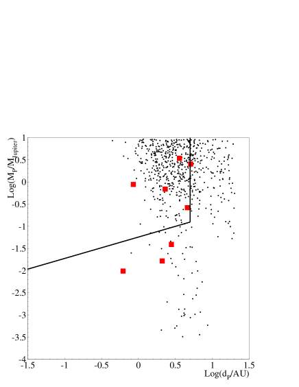
Figure 11: Scatter plot of the planet mass (in unit of Earth mass) vs planet distance (in Astronomical Units). The solid thick line delimits the region (upper and left) of planet detection accessible by radial velocities measurements with a precision up to 1 m s^-1. The observational data were accessed using the extrasolar planet on-line catalogue which collects the results of several collaborations (see http://exoplanet.eu/catalog.php and references therein). The eight small boxes are the planets detected by the microlensing technique. Starting from a sample of 40,000 detectable pixel-lensing events ($D=8$ m), 630 selected events (indicated by black dots) with $\chi_{\rm r}>4$, $N_{\rm good}>3$ and $\langle\epsilon\rangle_{\rm max}>0.1$ show planetary features and among these 48 events have $M_{\rm P}<20~{}M_{\oplus}$.

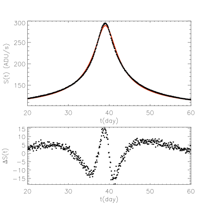
Figure 12: The upper panel shows the simulated light curve (black dots) of a planetary event with the parameters of the best fit model for the PA-99-N2 event (model W1 in Table 1 of An et al. 2004). In particular, $d=1.84$, $q=1.22\times 10^{-2}$ (corresponding to a planet mass $M_{\rm P}=6.34~{}M_{\rm{Jupiter}}$ for a disk lens of mass $M_{l}=0.5~{}M_{\odot}$), $u_{0}=3.4\times 10^{-2}$, $t_{\rm E}=132.3$ day and $\theta=24.5$ deg. We take the source magnitude $M_{\rm R}=-2.0$, and the source radius of $R_{s}=11~{}R_{\odot}$ (corresponding to $\rho=1.27\times 10^{-2}$ and $\rho/u_{0}=0.37$). It is also shown the best fit Paczyński like model modified for finite source effects (continuous line), which appears almost indistinguishable from the simulated data. The bottom panel gives the difference between the two curves. Here we use the INT telescope parameters and $N_{\rm im}=12$ day^-1.

The main result of the present work can be summarized in Fig. 11 ($D=8$ m), where for self-lensing events towards M31 with detectable planetary features we present the event scatter plot in the $(M_{\rm P},d_{\rm P})$ plane. The thick solid lines delimit the region (upper and left) where extrasolar planets are detectable by ground based observations, that are more sensitive to massive and close-in planets and that can be successfully applied only for systems close enough to Earth. We remind that current space based observations by Kepler and COROT satellites) are expected to decrease the minimum detectable planetary mass limit (up to one tenth of the Earth mass) and increase the planetary distance (up to tens of AUs). The eight extrasolar planets claimed so far to be detected by microlensing since 2003 in observations towards the Galactic bulge are represented by boxes. The locations of points in Fig. 11 show that the pixel-lensing technique may be used to search for extrasolar planets in M31 (including small mass planets), and at the moment this is the only method to discover planets in other galaxies. As one can see, detectable extrasolar planets have planet-to-star separations in the range $0.3-25$ AU and mass in the range $0.1~{}M_{\oplus}-10~{}M_{\rm{Jupiter}}$ (that coincides with the assumed lower and upper limits for planetary masses in the simulations). However, we note that the detection of planets with relative large masses is favourite (see also Fig. 7). We also caution that the planets with $M_{\rm P}<20~{}M_{\oplus}$ become undetectable and disappear from Fig. 11 if the adopted telescope has not a good enough photometric stability (about 0.03 mag, that is the required stability consistent with the typical error bars for the detection of small mass planets).

Before closing this section we note that an extrasolar planet in M31 might have been already detected since an anomaly in a pixel-lensing light curve has been reported (An et al., 2004). The authors claim that a binary system (lying on the M31 disk) with mass ratio $q=1.22\times 10^{-2}$ and distance $d=1.84$, is a possible explanation of the anomaly in the observed light curve. Other parameters are indicated in the caption of Fig. 12. In this figure we give a light curve with the best fit parameters of the PA-99-N2 event as given in Table 1 of An et al. (2004). It gives a clear deviation ($\chi_{\rm r}=49$, $\langle\epsilon\rangle_{\rm max}=0.6$) with respect to the corresponding Paczyński shape, at least with our ideal sampling of $N_{\rm im}=12$ day^-1 and observational conditions. In order to estimate the secondary object mass, we assume that the disk star mass follows the broken power law given by An et al. (2004). Accordingly, one finds a mean mass of $\simeq 0.5~{}M_{\odot}$ for the lens and therefore a mean value of $M_{\rm P}=6.34~{}M_{\rm{Jupiter}}$ for the planet. This value is at the boundary between the planet and brown dwarf region. Our light curve closely resembles the observed one and the basic characteristics of the planetary event fall in the parameter range for the II class of events.

5 Conclusions

We consider the possibility to detect planets in M31 by using pixel-lensing observations with telescopes of different sizes and observational strategies. This is the only way to detect planets in other galaxies and acquire information allowing a comparison of the planetary systems in M31 with respect to those in the Milky Way. We carry out MC simulations and explore the multi-dimensional space of the physical parameters of the planetary systems and characterize the sample of microlensing events for which the planet detections are more likely to be observed. We have assumed that each lens star in the M31 bulge and disk hosts one planet, and used for the planet mass distribution an simplified law, neglecting any dependence of the planet mass on the parent star mass and metallicity. Consideration of finite source effects induces a smoothening of the planetary deviations with respect to the point-like source approximation and, in turn, decreases the chance to detect planets. It also implies that in pixel-lensing searches towards M31 only few exposures per day could be enough to detect planetary features in light curves, at least when using large enough telescopes. We find that the pixel-lensing technique favours the detection of large mass planets ($M_{\rm P}\simeq 2~{}M_{\rm{Jupiter}}$), even if planets with mass less than $20~{}M_{\oplus}$ can be detected (with small probability, however) by using large telescopes with a sufficient photometric stability. Microlensing is intrinsically a ”no repetition” phenomenon and variable stars may mimic microlensing events and contaminate the sample of events attributed to microlensing. Therefore, real observations should be done at least in two bands, to check for achromaticity and be confident that the contamination by variables can be sorted out. However, a minor chromaticity is expected since the source limb darkening profile depends on the considered band and on the spectral type of the source star (see, e. g., Bogdanov & Cherepashchuk 1995b; Pejcha 2009).

Finally, we remark that although we have neglected the contribution to microlensing events of MACHOs in both galactic halos (in this respect the estimated planet rate should be considered as a lower bound), pixel-lensing observations towards M31 could be very useful in establishing whether planets may form around MACHOs as well.

References

- Alcock et al. (1993) Alcock, C., et al., 1993, Nature, 365, 621.
- An et al. (2004) An J.H., et al., 2004, ApJ, 601, 845.
- Ansari et al. (1997) Ansari, R., et al., 1997, A&A, 324, 843.
- Aparicio & Gallart (2004) Apparicio, A. & Gallart, C., 2004, AJ, 128, 1465.
- Baltz & Gondolo (2001) Baltz, E. A. & Gondolo, P., 2001, ApJ, 559, 41.
- Baillon et al. (1993) Baillon, P., Bouquet, A., Giraud-Heraud, Y. & Kaplan J., 1993, A&A, 277, 1.
- Beaulieu et al. (2006) Beaulieu, J.-P., et al. 2006, Nature, 439, 437.
- Bennett & Rhie (1996) Bennett, D. P. & Rhie, S. H., 1996, ApJ, 472, 660.
- Bennett (2009) Bennett, D. P., 2009, astro-ph/0902.1761.
- Bertelli et al. (1994) Bertelli, G., Bressan, A., Chiosi, C., Fagotto, F., Nasi. E., 1994, A&A SS, 106, 275.
- Bogdanov & Cherepashchuk (1995a) Bogdanov, M.B. & Cherepashchuk, A. M., 1995a, Astron. Rep. 39, 779.
- Bogdanov & Cherepashchuk (1995b) Bogdanov, M. V. & Cherepashchuk, A. M., 1995b, Astronomy Letters, 21, 505.
- Bolatto & Falco (1994) Bolatto, A. D. & Falco, E. E., 1994, ApJ, 436, 112.
- Bond et al. (2004) Bond, I. A., et al., 2004, ApJ, 606, L155.
- Bozza (1999) Bozza V., 1999, A&A, 348, 311.
- Calchi Novati et al. (2002) Calchi Novati S., et al., 2002, A&A, 381, 845.
- Calchi Novati et al. (2005) Calchi Novati S., et al., 2005, A&A, 443, 911.
- Calchi Novati et al. (2007) Calchi Novati S., et al., 2007, A&A, 469, 115.
- Calchi Novati et al. (2009) Calchi Novati S., et al., 2009, ApJ 695, 442.
- Chang & Refsdal (1984a) Chang, K. & Refsdal, S., 1984a, A&A, 132, 168.
- Chang & Refsdal (1984b) Chang, K. & Refsdal, S., 1984b, A&A, 139, 558.
- Chung et al. (2005) Chung, S.-J., et al., 2005, ApJ, 630, 535.
- Chung et al. (2006) Chung, S.-J., et al., 2006, ApJ, 650, 432.
- Claret (2000) Claret A., 2000, A&A, 363, 1081.
- Covone et al. (2000) Covone, G., de Ritis, R., Dominik, M. & Marino, A. A., 2000, A&A 357, 816.
- Crotts (1992) Crotts, A. P. S., 1992, ApJ, 399, L43.
- de Jong et al. (2006) de Jong, J. T. A., et al., 2006, A&A, 446, 855.
- De Paolis et al. (2005) De Paolis, F., Ingrosso, G., Nucita, A. A., Zakharov, A. F., 2005, A&A, 432, 501.
- Dominik (1999) Dominik, M., 1999, A&A 349, 108.
- Dominik (2005) Dominik, M., 2005, MNRAS 361, 300.
- Einstein (1936) Einstein, A., 1936, Science, 84, 506.
- Gaudi et al. (2008) Gaudi B. S., et al., 2008, Science, 319, 927.
- Gaudi & Gould (1997) Gaudi B. S. & Gould, A., 1997, ApJ, 486, 85.
- Gaudi & Gould (1999) Gaudi B. S. & Gould, A., 1999, ApJ, 513, 619.
- Girardi et al. (2002) Girardi, L., Bertelli, G., Bressan, A., Chiosi, C., Groenewegen, M. A. T., Marigo, P., Salasnich, B., Weiss, A., 2002, A&A, 391, 195.
- Gould (1996) Gould, A., 1996, ApJ, 470, 201.
- Gould & Loeb (1992) Gould A. & Loeb A. 1992, ApJ, 396, 104.
- Gould et al. (2006) Gould, A., et al., 2006, ApJ, 644, L37.
- Gould (2008) Gould, A., 2008, The Variable Universe: A Celebration of Bohdan Paczyński, ASP Conference Series, K. Stanek, ed., astro-ph/0803.4324.
- Griest & Safizadeh (1998) Griest, K. & Safizadeh N., 1998, ApJ, 500, 37.
- Han & Gaudi (2008) Han, C., & Gaudi 2008, astro-ph/0805.1103v1.
- Ida & Lin (2004) Ida, S. and Lin D.N.C., 2004, ApJ, 616, 567.
- Ingrosso et al. (2006) Ingrosso, G., Calchi Novati, S., De Paolis, F., Jetzer, Ph., Nucita, A. A., Strafella, F., 2006, A&A, 445, 375.
- Ingrosso et al. (2007) Ingrosso, G., Calchi Novati, S., De Paolis, F., Jetzer, Ph., Nucita, A. A., Scarpetta, G., Strafella, F., 2007, A&A, 462, 895.
- Johnson (2009) Johnson, J. A., 2009, astro-ph/0903.3059.
- Kerins et al. (2001) Kerins, E., et al., 2001, MNRAS, 323, 13.
- Kerins et al. (2006) Kerins, E., Darnley, M. J., Duke, J. P., Gould, A., Han, C., Jeon, Y.-B., Newsam, A., Park, B.-G., MNRAS, 365, 1099.
- Kim et al. (2007) Kim, D., et al., 2007, ApJ, 666, 236.
- Lineweaver & Grether (2003) Lineweaver, C.H. & Grether, D., 2003, ApJ, 598, 1350.
- Mao & Paczyński (1991) Mao, S., & Paczyński, B., 1991, ApJ, 374, L37.
- Mayor et al. (2009) Mayor, M., et al., 2009, A&A, manuscript GJ 581, in press.
- Paczyński (1986) Paczyński, B., 1986, ApJ, 304, 1.
- Paczyński (1996) Paczyński, B., 1996, ARA&A, 34, 419.
- Pejcha (2009) Pejcha, O. & Heyrovský, D., ApJ, 690, 1772.
- Perryman (2000) Perryman, M., 2000, Rep. Prog. Phys., 63, 1209.
- Perryman et al. (2005) Perryman, M., et al., 2005, Report by the ESA–ESO Working group on Extra-Solar Planets, astro-ph/0506163.
- Riffeser, Seitz & Bender (2008) Riffeser, A., Seitz S. & Bender R, 2008, ApJ, 684, 1093.
- Roulet & Mollerach (1997) Roulet, E. & Mollerach, S., 1997, Phys. Rep., 279, 2.
- Roulet & Mollerach (2002) Roulet, E. & Mollerach, S., 2002, Gravitational Lensing and Microlensing, World Scientific, Singapore.
- Schneider, Ehlers & Falco (1992) Schneider, P., Ehlers, J. & Falco E. E., 1992, Gravitational Lensing, Springer, Berlin.
- Schneider & Weiss (1992) Schneider, P. & Weiss, A., 1992, A&A, 260, 1.
- Tabachnik & Tremaine (2002) Tabachnik S., & Tremaine S., 2002, MNRAS, 335, 151.
- Witt (1990) Witt, H. J., 1990, A&A, 236, 311.
- Witt & Mao (1994) Witt, H. J., & Mao, S., 1994, ApJ, 430, 505.
- Witt & Mao (1995) Witt, H. J., & Mao, S., 1995, ApJ, 447, L105.
- Udalski et al. (2005) Udalski, A., et al., 2005, ApJ 628, L109.
- Udry & Santos (2007) Udry, S. & Santos, N.C. 2007, ARA&A 45, 397.
- Zakharov & Sazhin (1995) Zakharov, A.F. & Sazhin, M.V., 1995, A & A 293, 1.
- Zakharov & Sazhin (1997a) Zakharov A.F. & Sazhin, M.V., 1997a, Astron. Rep. 74, 336.
- Zakharov & Sazhin (1997b) Zakharov A.F. & Sazhin, M.V., 1997b, Astron. Lett. 23, 937.
- Zakharov & Sazhin (1998) Zakharov A.F. & Sazhin, M.V., 1998, Physics – Uspekhi 41, 945.