Applications of Stein’s method for concentration inequalities

Abstract

Stein’s method for concentration inequalities was introduced to prove concentration of measure in problems involving complex dependencies such as random permutations and Gibbs measures. In this paper, we provide some extensions of the theory and three applications: (1) We obtain a concentration inequality for the magnetization in the Curie–Weiss model at critical temperature (where it obeys a nonstandard normalization and super-Gaussian concentration). (2) We derive exact large deviation asymptotics for the number of triangles in the Erdős–Rényi random graph $G(n,p)$ when $p\geq 0.31$. Similar results are derived also for general subgraph counts. (3) We obtain some interesting concentration inequalities for the Ising model on lattices that hold at all temperatures.

and

t1Supported in part by NSF Grant DMS-07-07054 and a Sloan Research Fellowship.

60E15, 60F10, 60C05, 82B44, Stein’s method, Gibbs measures, concentration inequality, Ising model, Curie–Weiss model, large deviation, Erdos–Renyi random graph, exponential random graph

1 Introduction

In his seminal 1972 paper stein72 , Charles Stein introduced a method for proving central limit theorems with convergence rates for sums of dependent random variables. This has now come to be known as Stein’s method. The technique is primarily used for proving distributional limit theorems (both Gaussian and non-Gaussian). Stein’s attempts stein86 at devising a version of the method for large deviations did not prove fruitful. Some progress for sums of dependent random variables was made by Raič raic04 . The problem was finally solved in full generality in chatterjee05 . A selection of results and examples from chatterjee05 appeared in the later papers chatterjee07 , chatterjee07a . In this paper, we extend the theory and work out three further examples. The paper is fully self-contained.

The sections are organized as follows. In Section 2, we state the main results, the examples, and some proof sketches. The complete proofs are in Section 3.

2 Results and examples

The following abstract theorem is quotedfrom chatterjee07 . It summarizes a collection of results from chatterjee05 . This is a generalization of Stein’s method of exchangeable pairs to the realm of concentration inequalities and large deviations.

Theorem 1 ((chatterjee07 , Theorem 1.5))

Let $\mathcal{X}$ be a separable metric space and suppose $(X,X^{\prime})$ is an exchangeable pair of $\mathcal{X}$-valued random variables. Suppose $f\dvtx\mathcal{X}\to\mathbb{R}$ and $F\dvtx\mathcal{X}\times\mathcal{X}\to\mathbb{R}$ are square-integrable functions such that $F$ is antisymmetric [i.e., $F(X,X^{\prime})=-F(X^{\prime},X)$ a.s.], and $\mathbb{E}(F(X,X^{\prime})|X)=f(X)$ a.s. Let

$$\Delta(X):=\tfrac{1}{2}\mathbb{E}\bigl{(}\bigl{|}\bigl{(}f(X)-f(X^{\prime})\bigr{)}F(X,X^{\prime})\bigr{|}|X\bigr{)}.$$

Then $\mathbb{E}(f(X))=0$, and the following concentration results hold for $f(X)$:

If $\mathbb{E}(\Delta(X))<\infty$, then $\operatorname{Var}(f(X))=\frac{1}{2}\mathbb{E}((f(X)-f(X^{\prime}))F(X,X^{\prime}))$.

Assume that $\mathbb{E}(e^{\theta f(X)}|F(X,X^{\prime})|)<\infty$ for all $\theta$. If there exists nonnegative constants $B$ and $C$ such that $\Delta(X)\leq Bf(X)+C$ almost surely, then for any $t\geq 0$,

$$\mathbb{P}\{f(X)\geq t\}\leq\exp\biggl{(}-\frac{t^{2}}{2C+2Bt}\biggr{)}\quad\mbox{and}\quad\mathbb{P}\{f(X)\leq-t\}\leq\exp\biggl{(}-\frac{t^{2}}{2C}\biggr{)}.$$

For any positive integer $k$, we have the following exchangeable pairs version of the Burkholder–Davis–Gundy inequality:

$$\mathbb{E}(f(X)^{2k})\leq(2k-1)^{k}\mathbb{E}(\Delta(X)^{k}).$$

Note that the finiteness of the exponential moment for all $\theta$ ensures that the tail bounds hold for all $t$. If it is finite only in a neighborhood of zero, the tail bounds will hold for $t$ less than a threshold.

One of the contributions of the present paper is the following generalization of the above result for non-Gaussian tail behavior. We apply it to obtain a concentration inequality with the correct tail behavior in the Curie–Weiss model at criticality.

Theorem 2

Suppose $(X,X^{\prime})$ is an exchangeable pair of random variables. Let $F(X,X^{\prime}),f(X)$ and $\Delta(X)$ be as in Theorem 1. Suppose that we have

$$\Delta(X)\leq\psi(f(X))\qquad\mbox{almost surely}$$

for some nonnegative symmetric function $\psi$ on $\mathbb{R}$. Assume that $\psi$ is nondecreasing and twice continuously differentiable in $(0,\infty)$ with

$$\alpha:=\sup_{x>0}x\psi^{\prime}(x)/\psi(x)<2$$ (1)

and

$$\delta:=\sup_{x>0}x\psi^{\prime\prime}(x)/\psi(x)<\infty.$$ (2)

Assume that $\mathbb{E}(|f(X)|^{k})<\infty$ for all positive integer $k\geq 1$. Then for any $t\geq 0$, we have

$$\mathbb{P}\bigl{(}|f(X)|>t\bigr{)}\leq c\exp\biggl{(}-\frac{t^{2}}{2\psi(t)}\biggr{)}$$

for some constant $c$ depending only on $\alpha,\delta$. Moreover, if $\psi$ is only once differentiable with $\alpha<2$ as in (1), then the tail inequality holds with exponent $t^{2}/4\psi(t)$.

An immediate corollary of Theorem 2 is the following.

Corollary 3

Suppose $(X,X^{\prime})$ is an exchangeable pair of random variables. Let $F(X,X^{\prime}),f(X)$ and $\Delta(X)$ be as in Theorem 1. Suppose that for some real number $\alpha\in(0,2)$ we have

$$\Delta(X)\leq B|f(X)|^{\alpha}+C\qquad\mbox{almost surely},$$

where $B>0,C\geq 0$ are constants. Assume that $\mathbb{E}(|f(X)|^{k})<\infty$ for all positive integer $k\geq 1$. Then for any $t\geq 0$ we have

$$\mathbb{P}\bigl{(}|f(X)|>t\bigr{)}\leq c_{\alpha}\exp\biggl{(}-\frac{1}{2}\cdot\frac{t^{2}}{Bt^{\alpha}+C}\biggr{)}$$

for some constant $c_{\alpha}$ depending only on $\alpha$.

The result in Theorem 2 states that the tail behavior of $f(X)$ is essentially given by the behavior of $f(X)^{2}/\Delta(X)$. Condition (1) implies that $\psi(x)<\psi(1)(1+x^{2})$ for all $x\in\mathbb{R}$. Moreover, the constant $c_{\alpha}$ appearing in Theorem 2 can be written down explicitly but we did not attempt to optimize the constant. The proof of Theorem 2 is along the same lines as Theorem 1, but somewhat more involved. Deferring the proof to Section 3, let us move on to examples.

2.1 Example: Curie–Weiss model at criticality

The “Curie–Weiss model of ferromagnetic interaction” at inverse temperature $\beta$ and zero external field is given by the following Gibbs measure on $\{+1,-1\}^{n}$. For a typical configuration $\bolds{\sigma}=(\sigma_{1},\sigma_{2},\ldots,\sigma_{n})\in\{+1,-1\}^{n}$, the probability of $\bolds{\sigma}$ is given by

$$\mu_{\beta}(\{\bolds{\sigma}\}):=Z_{\beta}^{-1}\exp\biggl{(}\frac{\beta}{n}\sum_{i<j}\sigma_{i}\sigma_{j}\biggr{)},$$

where $Z_{\beta}=Z_{\beta}(n)$ is the normalizing constant. It is well known that the Curie–Weiss model shows a phase transition at $\beta_{c}=1$. For $\beta<\beta_{c}$, the magnetization $m(\bolds{\sigma}):=\frac{1}{n}\sum_{i=1}^{n}\sigma_{i}$ is concentrated at $0$ but for $\beta>\beta_{c}$ the magnetization is concentrated on the set $\{-x^{*},x^{*}\}$ where $x^{*}>0$ is the largest solution of the equation $x=\tanh(\beta x)$. In fact, using concentration inequalities for exchangeable pairs it was proved in chatterjee05 (Proposition 1.3) that for all $\beta\geq 0,h\in\mathbb{R},n\geq 1,t\geq 0$ we have

$$\mathbb{P}\biggl{(}|m-\tanh(\beta m+h)|\geq\frac{\beta}{n}+\frac{t}{\sqrt{n}}\biggr{)}\leq 2\exp\biggl{(}-\frac{t^{2}}{4(1+\beta)}\biggr{)},$$

where $h$ is the external field, which is zero in our case. Although a lot is known about this model (see Ellis ellis85 , Section IV.4, for a survey), the above result—to the best of our knowledge—is the first rigorously proven concentration inequality that holds at all temperatures. (See also chazottes06 for some related results.)

Incidentally, the above result shows that when $\beta<1$, the magnetization is at most of order $n^{-1/2}$. It is known that at the critical temperature the magnetization $m(\bolds{\sigma})$ shows a non-Gaussian behavior and is of order $n^{-1/4}$. In fact, at $\beta=1$ as $n\to\infty$, $n^{1/4}m(\bolds{\sigma})$ converges to the probability distribution on $\mathbb{R}$ having density proportional to $\exp(-t^{4}/12)$. This limit theorem was first proved by Simon and Griffiths simon73 and error bounds were obtained recently chatterjeeshao09 , eichelsbacherlowe09 . The following concentration inequality, derived using Theorem 2, fills the gap in the tail bound at the critical point.

Proposition 4

Suppose $\bolds{\sigma}$ is drawn from the Curie–Weiss model at the critical temperature $\beta=1$. Then, for any $n\geq 1$ and $t\geq 0$, the magnetization satisfies

$$\mathbb{P}\bigl{(}n^{1/4}|m(\bolds{\sigma})|\geq t\bigr{)}\leq 2e^{-ct^{4}},$$

where $c>0$ is an absolute constant.

Here, we may remark that such a concentration inequality probably cannot be obtained by application of standard off-the-shelf results (e.g., those surveyed in Ledoux ledoux01 , the famous results of Talagrand talagrand95 or the recent breakthroughs of Boucheron, Lugosi and Massart blm03 ), because they generally give Gaussian or exponential tail bounds. There are several recent remarkable results giving tail bounds different from exponential and Gaussian. The papers bcr06 , lo00 , ggm05 , chazottes06 deal with tails between exponential and Gaussian and bcr05 , bob07 deal with subexponential tails. Also in bl00 , gozlan07 , gozlan09 , the authors deal with tails (possibly) larger than Gaussian. However, it seems that none of the techniques given in these references would lead to the result of Proposition 4.

It is possible to derive a similar tail bound using the asymptotic results of Martin-Löf martinlof82 about the partition function $Z_{\beta}(n)$ (see also Bolthausen bolthausen87 ). An application of their results gives that

$$\sum_{\bolds{\sigma}\in\{-1,+1\}^{n}}e^{{n}/{2}m(\bolds{\sigma})^{2}+n\theta m(\bolds{\sigma})^{4}}\simeq\frac{2^{n+1}\Gamma(5/4)}{\sqrt{2\pi}}\biggl{(}\frac{12n}{1-12\theta}\biggr{)}^{1/4}$$

for $\theta<1/12$ in the sense that the ratio of the two sides converges to one as $n$ goes to infinity and from here the tail bound follows easily (without an explicit constant). However, this approach depends on a precise estimate of the partition function [e.g., large deviation estimates or finding the limiting free energy $\lim n^{-1}\log Z_{\beta}(n)$ are not enough] and this precise estimate is hard to prove. Our method, on the other hand, depends only on simple properties of the Gibbs measure and is not tied specifically to the Curie–Weiss model.

The idea used in the proof of Proposition 4 can be used to prove a tail inequality that holds for all $0\leq\beta\leq 1$. We state the result below without proof. Note that the inequality gives the correct tail bound for all $0\leq\beta\leq 1$.

Proposition 5

Suppose $\bolds{\sigma}$ is drawn from the Curie–Weiss model at inverse temperature $\beta$ where $0\leq\beta\leq 1$. Then, for any $n\geq 1$ and $t\geq 0$ the magnetization satisfies

$$\mathbb{P}\bigl{(}3(1-\beta)m(\bolds{\sigma})^{2}+\beta^{3}m(\bolds{\sigma})^{4}\geq t\bigr{)}\leq 2e^{-nt/160}.$$

It is possible to derive similar non-Gaussian tail inequalities for general Curie–Weiss models at the critical temperature. We briefly discuss the general case below. Let $\rho$ be a symmetric probability measure on $\mathbb{R}$ with $\int x^{2}\,d\rho(x)=1$ and $\int\exp(\beta x^{2}/2)\,d\rho(x)<\infty$ for all $\beta\geq 0$. The general Curie–Weiss model CW$(\rho)$ at inverse temperature $\beta$ is defined as the array of spin random variables $\mathbf{X}=(X_{1},X_{2},\ldots,X_{n})$ with joint distribution

$$d\nu_{n}(\mathbf{x})=Z_{n}^{-1}\exp\biggl{(}\frac{\beta}{2n}(x_{1}+x_{2}+\cdots+x_{n})^{2}\biggr{)}\prod_{i=1}^{n}d\rho(x_{i})$$ (3)

for $\mathbf{x}=(x_{1},x_{2},\ldots,x_{n})\in\mathbb{R}^{n}$ where

$$Z_{n}=\int\exp\biggl{(}\frac{\beta}{2n}(x_{1}+x_{2}+\cdots+x_{n})^{2}\biggr{)}\prod_{i=1}^{n}d\rho(x_{i})$$

is the normalizing constant. The magnetization $m(\mathbf{x})$ is defined as usual by $m(\mathbf{x})=n^{-1}\sum_{i=1}^{n}x_{i}$. Here, we will consider the case when $\rho$ satisfies the following two conditions:

1. [(B)]

2. $\rho$ has compact support, that is, $\rho([-L,L])=1$ for some $L<\infty$.

3. The equation $h^{\prime}(s)=0$ has a unique root at $s=0$ where

   $$h(s):=\frac{s^{2}}{2}-\log\int\exp(sx)\,d\rho(x)\qquad\mbox{for }s\in\mathbb{R}.$$

The second condition says that $h(\cdot)$ has a unique global minima at $s=0$ and $|h^{\prime}(s)|>0$ for $|s|>0$. The behavior of this model is quite similar to the classical Curie–Weiss model and there is a phase transition at $\beta=1$. For $\beta<1$, $m(\mathbf{X})$ is concentrated around zero while for $\beta>1,m(\mathbf{X})$ is bounded away from zero a.s. (see Ellis and Newman ellis78 , ellis78a ). We will prove the following concentration result.

Proposition 6

Suppose $\mathbf{X}\sim\nu_{n}$ at the critical temperature $\beta=1$ where $\rho$ satisfies conditions (A) and (B). Let $k$ be such that $h^{(i)}(0)=0$ for $0\leq i<2k$ and $h^{(2k)}(0)\neq 0$, where

$$h(s):=\frac{s^{2}}{2}-\log\int\exp(sx)\,d\rho(x)\qquad\mbox{for }s\in\mathbb{R},$$

and $h^{(i)}$ is the $i$th derivative of $h$. Then, $k>1$ and for any $n\geq 1$ and $t\geq 0$ the magnetization satisfies

$$\mathbb{P}\bigl{(}n^{1/2k}|m(\mathbf{X})|\geq t\bigr{)}\leq 2e^{-ct^{2k}},$$

where $c>0$ is an absolute constant depending only on $\rho$.

Here, we mention that in Ellis and Newman ellis78 , convergence results were proved for the magnetization in CW$(\rho)$ model under optimal condition on $\rho$. Under our assumption, their result says that $n^{1/2k}m(\mathbf{X})$ converges weakly to a distribution having density proportional to $\exp(-\lambda x^{2k}/(2k)!)$ where $\lambda:=h^{(2k)}(0)$. Hence, the tail bound gives the correct convergence rate.

Let us now give a brief sketch of the proof of Proposition 4. Suppose $\bolds{\sigma}$ is drawn from the Curie–Weiss model at the critical temperature. We construct $\bolds{\sigma}^{\prime}$ by taking one step in the heat-bath Glauber dynamics: a coordinate $I$ is chosen uniformly at random, and $\sigma_{I}$ is replace by $\sigma^{\prime}_{I}$ drawn from the conditional distribution of the $I$th coordinate given $\{\sigma_{j}\dvtx j\neq I\}$. Let

$$F(\bolds{\sigma},\bolds{\sigma}^{\prime}):=\sum_{i=1}^{n}(\sigma_{i}-\sigma^{\prime}_{i})=\sigma_{I}-\sigma^{\prime}_{I}.$$

For each $i=1,2,\ldots,n$, define $m_{i}=m_{i}(\bolds{\sigma})=n^{-1}\sum_{j\neq i}\sigma_{j}.$ An easy computaion gives that $\mathbb{E}(\sigma_{i}|\{\sigma_{j},j\neq i\})=\tanh(m_{i})$ for all $i$ and so we have

$$f(\bolds{\sigma}):=\mathbb{E}(F(\bolds{\sigma},\bolds{\sigma}^{\prime})|\bolds{\sigma})=m-\frac{1}{n}\sum_{i=1}^{n}\tanh(m_{i})=\frac{m}{n}+\frac{1}{n}\sum_{i=1}^{n}g(m_{i}),$$

where $g(x):=x-\tanh(x)$. Note that $|m_{i}-m|\leq 1/n$, and hence $f(\bolds{\sigma})=m-\tanh m+O(1/n)$. A simple analytical argument using the fact that, for $x\approx 0$, $x-\tanh x=x^{3}/3+O(x^{5})$ then gives

$$\Delta(\bolds{\sigma})\leq\frac{6}{n}|f(\bolds{\sigma})|^{2/3}+\frac{12}{n^{5/3}}$$

and using Corollary 3 with $\alpha=2/3,B=6/n$ and $C=12/n^{5/3}$ we have

$$\mathbb{P}(|m-\tanh m|\geq t+n^{-1})\leq\mathbb{P}\bigl{(}|f(\bolds{\sigma})|\geq t\bigr{)}\leq 2e^{-cnt^{4/3}}$$

for all $t\geq 0$ for some constant $c>0$. It is easy to see that this implies the result. The critical observation, of course, is that $x-\tanh(\beta x)=O(x^{3})$ for $\beta=1$, which is not true for $\beta\neq 1$.

2.2 Example: Triangles in Erdős–Rényi graphs

Consider the Erdős–Rényi random graph model $G(n,p)$ which is defined as follows. The vertex set is $[n]:=\{1,2,\ldots,n\}$ and each edge $(i,j),1\leq i<j\leq n$, is present with probability $p$ and not present with probability $1-p$ independently of each other. For any three distinct vertex $i<j<k$ in $[n]$ we say that the triple $(i,j,k)$ forms a triangle in the graph $G(n,p)$ if all the three edges $(i,j),(j,k),(i,k)$ are present in $G(n,p)$ (see Figure 1). Let $T_{n}$ be the number of triangles in $G(n,p)$, that is,

$$T_{n}:=\sum_{1\leq i<j<k\leq n}\mathbf{1}\{(i,j,k)\mbox{ forms a triangle in }G(n,p)\}.$$

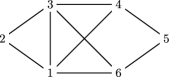
Figure 1: A graph on $6$ vertices with $8$ edges and $3$ triangles. The triangles being $(1,2,3),(1,3,4)$ and $(1,3,6)$.

Let us define the function $I(\cdot,\cdot)$ on $(0,1)\times(0,1)$ as

$$I(r,s):=r\log\frac{r}{s}+(1-r)\log\frac{1-r}{1-s}.$$ (4)

Note that $I(r,s)$ is the Kullback–Leibler divergence of the measure $\nu_{s}$ from $\nu_{r}$ and also the relative entropy of $\nu_{r}$ w.r.t. $\nu_{s}$ where $\nu_{p}$ is the Bernoulli$(p)$ measure. We have the following result about the large deviation rate function for the number of triangles in $G(n,p)$.

Theorem 7

Let $T_{n}$ be the number of triangles in $G(n,p)$, where $p>p_{0}$ where $p_{0}=2/(2+e^{3/2})\approx 0.31$. Then for any $r\in(p,1]$,

$$\mathbb{P}\left(T_{n}\geq\pmatrix{n\cr 3}r^{3}\right)=\exp\biggl{(}-\frac{n^{2}I(r,p)}{2}\bigl{(}1+O(n^{-1/2})\bigr{)}\biggr{)}.$$ (5)

Moreover, even if $p\leq p_{0}$, there exist $p^{\prime},p^{\prime\prime}$ such that $p<p^{\prime}\leq p^{\prime\prime}<1$ and the same result holds for all $r\in(p,p^{\prime})\cup(p^{\prime\prime},1]$. For all $p$ and $r$ in the above domains, we also have the more precise estimate

$$\quad\mathbb{P}\left(\left|T_{n}-\pmatrix{n\cr 3}r^{3}\right|\leq C(p,r)n^{5/2}\right)=\exp\biggl{(}-\frac{n^{2}I(r,p)}{2}\bigl{(}1+O(n^{-1/2})\bigr{)}\biggr{)},$$ (6)

where $C(p,r)$ is a constant depending on $p$ and $r$.

The behavior of the upper tail of subgraph counts in $G(n,p)$ is a problem of great interest in the theory of random graphs (see bollobas85 , jansonetal00 , jansonrucinski02 , vu01 , kimvu04 , and references contained therein). The best upper bounds to date were obtained by Kim and Vu kimvu04 (triangles) and Janson, Oleszkiewicz, and Ruciński jansonolesz04 (general subgraph counts). For triangles, the results of these papers essentially state that for a fixed $\epsilon>0$,

$$\exp\bigl{(}-\Theta\bigl{(}n^{2}p^{2}\log(1/p)\bigr{)}\bigr{)}\leq\mathbb{P}\bigl{(}T_{n}\geq\mathbb{E}(T_{n})+\epsilon n^{3}p^{3}\bigr{)}\leq\exp(-\Theta(n^{2}p^{2})).$$

Clearly, our result gives a lot more in the situations where it works (see Figure 2). The method of proof can be easily extended to prove similar results for general subgraph counts and are discussed in Section 2.3. However, there is an obvious incompleteness in Theorem 7 (and also for general subgraphs counts), namely, that it does not work for all $(p,r)$.

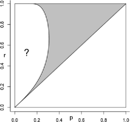
Figure 2: The set (colored in gray) of $(p,r),r\geq p$, for which we are able to show that the large deviation result holds.

In this context, we should mention that another paper on large deviations for subgraph counts by Bolthausen, Comets and Dembo bolthausenetal09 is in preparation. As of now, to the best of our knowledge, the authors of bolthausenetal09 have only looked at subgraphs that do not complete loops, like $2$-stars. Another related article is the one by Döring and Eichelsbacher doringeichelsbacher09 , who obtain moderate deviations for a class of graph-related objects, including triangles.

Unlike the previous two examples, Theorem 7 is far from being a direct consequence of any of our abstract results. Therefore, let us give a sketch of the proof, which involves a new idea.

The first step is standard: consider tilted measures. However, the appropriate tilted measure in this case leads to what is known as an “exponential random graph,” a little studied object in the rigorous literature. Exponential random graphs have become popular in the statistical physics and network communities in recent years (see the survey of Park and Newman parknewman04 ). The only rigorous work we are aware of is the recent paper of Bhamidi et al. bhamidi08 , who look at convergence rates of Markov chains that generate such graphs.

We will not go into the general definition or properties of exponential random graphs. Let us only define the model we need for our purpose.

Fix two numbers $\beta\geq 0$ and $h\in\mathbb{R}$. Let $\Omega=\{0,1\}^{n\choose 2}$ be the space of all tuples like $\mathbf{x}=(x_{ij})_{1\leq i<j\leq n}$, where $x_{ij}\in\{0,1\}$ for each $i,j$. Let $\mathbf{X}=(X_{ij})_{1\leq i<j\leq n}$ be a random element of $\Omega$ following the probability measure proportional to $e^{H(\mathbf{x})}$, where $H$ is the Hamiltonian:

$$H(\mathbf{x})=\frac{\beta}{n}\sum_{1\leq i<j<k\leq n}x_{ij}x_{jk}x_{ik}+h\sum_{1\leq i<j\leq n}x_{ij}.$$

Note that any element of $\Omega$ naturally defines an undirected graph on a set of $n$ vertices. For each $\mathbf{x}\in\Omega$, let $T(\mathbf{x})=\sum_{i<j<k}x_{ij}x_{jk}x_{ik}$ denote the number of triangles in the graph defined by $\mathbf{x}$, and let $E(\mathbf{x})=\sum_{i<j}x_{ij}$ denote the number of edges. Then the above Hamiltonian is nothing but

$$\frac{\beta T(\mathbf{x})}{n}+hE(\mathbf{x}).$$

For notational convenience, we will assume that $x_{ij}=x_{ji}$. Let $Z_{n}(\beta,h)$ be the corresponding partition function, that is,

$$Z_{n}(\beta,h)=\sum_{\mathbf{x}\in\Omega}e^{H(\mathbf{x})}.$$

Note that $\beta=0$ corresponds to the Erdős–Rényi random graph with $p=e^{h}/(1+e^{h})$. The following theorem “solves” this model in a “high temperature region.” Once this solution is known, the computation of the large deviation rate function is just one step away.

Theorem 8 ((Free energy in high temperature regime))

Suppose we have $\beta\geq 0$, $h\in\mathbb{R}$, and $Z_{n}(\beta,h)$ defined as above. Define a function $\varphi\dvtx[0,1]\to\mathbb{R}$ as

$$\varphi(x)=\frac{e^{\beta x+h}}{1+e^{\beta x+h}}.$$

Suppose $\beta$ and $h$ are such that the equation $u=\varphi(u)^{2}$ has a unique solution $u^{*}$ in $[0,1]$ and $2\varphi(u^{*})\varphi^{\prime}(u^{*})<1$. Then

$$\lim_{n\to\infty}\frac{\log Z_{n}(\beta,h)}{n^{2}}=-\frac{1}{2}I(\varphi(u^{*}),\varphi(0))-\frac{1}{2}\log\bigl{(}1-\varphi(0)\bigr{)}+\frac{\beta\varphi(u^{*})^{3}}{6},$$

where $I(\cdot,\cdot)$ is the function defined in (4). Moreover, there exists a constant $K(\beta,h)$ that depends only on $\beta$ and $h$ (and not on $n$) such that difference between $n^{-2}\log Z_{n}(\beta,h)$ and the limit is bounded by $K(\beta,h)n^{-1/2}$ for all $n$.

Incidentally, the above solution was obtained using physical heuristics by Park and Newman parknewman05 in 2005. Here, we mention that, in fact, the following result is always true.

Lemma 9

For any $\beta\geq 0,h\in\mathbb{R}$, we have

$$\liminf_{n\to\infty}\frac{\log Z_{n}(\beta,h)}{n^{2}}$$

$$\qquad\geq\sup_{r\in(0,1)}\biggl{\{}-\frac{1}{2}I(r,\varphi(0))-\frac{1}{2}\log\bigl{(}1-\varphi(0)\bigr{)}+\frac{\beta r^{3}}{6}\biggr{\}}$$ (7)

$$\qquad=\sup_{u\dvtx\varphi(u)^{2}=u}\biggl{\{}-\frac{1}{2}I(\varphi(u),\varphi(0))-\frac{1}{2}\log\bigl{(}1-\varphi(0)\bigr{)}+\frac{\beta\varphi(u)^{3}}{6}\biggr{\}}.$$

We will characterize the set of $\beta,h$ for which the conditions in Theorem 8 hold in Lemma 12. First of all, note that the appearance of the function $\varphi(u)^{2}-u$ is not magical. For each $i<j$, define

$$L_{ij}=\frac{1}{n}\sum_{k\notin\{i,j\}}X_{ik}X_{jk}.$$

This is the number of “wedges” or $2$-stars in the graph that have the edge $ij$ as base. The key idea is to use Theorem 1 to show that these quantities approximately satisfy the following set of “mean field equations”:

$$L_{ij}\simeq\frac{1}{n}\sum_{k\notin\{i,j\}}\varphi(L_{ik})\varphi(L_{jk})\qquad\mbox{for all }i<j.$$ (8)

(The idea of using Theorem 1 to prove mean field equations was initially developed in Section 3.4 of chatterjee05 .) The following lemma makes this notion precise. Later, we will show that under the conditions of Theorem 8, this system has a unique solution.

Lemma 10 ((Mean field equations))

Let $\varphi$ be defined as in Theorem 8. Then for any $1\leq i<j\leq n$, we have

$$\mathbb{P}\biggl{(}\sqrt{n}\biggl{|}L_{ij}-\frac{1}{n}\sum_{k\notin\{i,j\}}\varphi(L_{ik})\varphi(L_{jk})\biggr{|}\geq t\biggr{)}\leq 2\exp\biggl{(}-\frac{t^{2}}{8(1+\beta)}\biggr{)}$$

for all $t\geq 8\beta/n$. In particular, we have

$$\mathbb{E}\biggl{|}L_{ij}-\frac{1}{n}\sum_{k\notin\{i,j\}}\varphi(L_{ik})\varphi(L_{jk})\biggr{|}\leq\frac{C(1+\beta)^{1/2}}{n^{1/2}},$$ (9)

where $C$ is a universal constant.

In fact, one would expect that $L_{ij}\simeq u^{*}$ for all $i<j$, if the equation

$$\psi(u):=\varphi(u)^{2}-u=0$$ (10)

has a unique solution $u^{*}$ in $[0,1]$. The intuition behind is as follows. Define $L_{\max}=\max_{i,j}L_{ij}$ and $L_{\min}=\min_{i,j}L_{ij}$. It is easy to see that $\varphi$ is an increasing function. Hence, from the mean-field equations (8), we have $L_{\max}\leq\varphi(L_{\max})^{2}+o(1)$ or $\psi(L_{\max})\geq o(1)$. But $\psi(u)\geq 0$ iff $u\leq u^{*}$. Hence, $L_{\max}\leq u^{*}+o(1)$. Similarly, we have $L_{\min}\geq u^{*}-o(1)$ and thus all $L_{ij}\simeq u^{*}$. Lemma 11 formalizes this idea. Here, we mention that one can easily check that equation (10) has at most three solutions. Moreover, $\psi(0)>0>\psi(1)$ implies that $\psi^{\prime}(u^{*})\leq 0$ or $2\varphi(u^{*})\varphi^{\prime}(u^{*})\leq 1$ if $u^{*}$ is the unique solution to (10).

Lemma 11

Let $u^{*}$ be the unique solution of the equation $u=\varphi(u)^{2}$. Assume that $2\varphi(u^{*})\varphi^{\prime}(u^{*})<1$. Then for each $1\leq i<j\leq n$, we have

$$\mathbb{E}|L_{ij}-u^{*}|\leq\frac{K(\beta,h)}{n^{1/2}},$$

where $K(\beta,h)$ is a constant depending only on $\beta,h$. Moreover, if $2\varphi(u^{*})\varphi^{\prime}(u^{*})=1$ then we have

$$\mathbb{E}|L_{ij}-u^{*}|\leq\frac{K(\beta,h)}{n^{1/6}}\qquad\mbox{for all }1\leq i<j\leq n.$$

Now observe that the Hamiltonian $H(\mathbf{X})$ can be written as

$$H(\mathbf{X})=\frac{\beta}{6}\sum_{1\leq i<j\leq n}X_{ij}L_{ij}+h\sum_{1\leq i<j\leq n}X_{ij}.$$

The idea then is the following: once we know that the conclusion of Lemma 11 holds, each $L_{ij}$ in the above Hamiltonian can be replaced by $u^{*}$, which results in a model where the coordinates are independent. The resulting probability measure is presumably quite different from the original measure, but somehow the partition functions remain comparable.

The following lemma (Lemma 12) characterizes the region $S\in\mathbb{R}\times[0,\infty)$ such that the equation $u=\varphi(u)^{2}$ has a unique solution $u^{*}$ in $[0,1]$ and $2\varphi(u^{*})\varphi^{\prime}(u^{*})<1$ for $(h,\beta)\in S$ (see Figure 3).

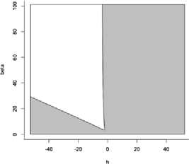
Figure 3: The set $S$ (colored in gray) of $(h,\beta)$ for which the conditions of Theorem 8 hold.

Let $h_{0}=\log 2-\frac{3}{2}<0$. For $h<h_{0}$ there exist exactly two solutions $0<a_{*}=a_{*}(h)<1/2<a^{*}=a^{*}(h)<\infty$ to the equation

$$\log x+\frac{1+x}{2x}+h=0.$$

Define $a_{*}(h)=a^{*}(h)=1/2$ for $h=h_{0}$ and

$$\beta_{*}(h)=\frac{(1+a_{*})^{3}}{2a_{*}}\quad\mbox{and}\quad\beta^{*}(h)=\frac{(1+a^{*})^{3}}{2a^{*}}$$ (11)

for $h\leq h_{0}$.

Lemma 12 ((Characterization of high temperature regime))

Let $S$ be the set of pairs $(h,\beta)$ for which the function $\psi(u):=\varphi(u)^{2}-u$ has a unique root $u^{*}$ in $[0,1]$ and $2\varphi(u^{*})\varphi^{\prime}(u^{*})<1$ where $\varphi(u):=e^{\beta u+h}/(1+e^{\beta u+h}).$ Then we have

$$S^{c}=\{(h,\beta)\dvtx h\leq h_{0}\mbox{ and }\beta_{*}(h)\leq\beta\leq\beta^{*}(h)\},$$

where $\beta^{*},\beta_{*}$ are as given in equation (11). In particular, $(h,\beta)\in S$ if $\beta\leq(3/2)^{3}$ or $h>h_{0}$.

The point $h=h_{0},\beta=\beta_{0}:=(3/2)^{3}$ is the critical point and the curve

$$\gamma(t)=\biggl{(}-\log t-\frac{1+t}{2t},\frac{(1+t)^{3}}{2t}\biggr{)}$$ (12)

for $t>0$ is the phase transition curve. It corresponds to $\psi(u^{*})=0$ and $2\psi(u^{*})\psi^{\prime}(u^{*})=1$. In fact, at the critical point $(h_{0},\beta_{0})$ the function $\psi(u)=\varphi(u)^{2}-u$ has a unique root of order three at $u^{*}=4/9$, that is, $\psi(u^{*})=\psi^{\prime}(u^{*})=\psi^{\prime\prime}(u^{*})=0$ and $\psi^{\prime\prime\prime}(u^{*})<0$. The second part of Lemma 11 shows that all the above conclusions (including the limiting free energy result) are true for the critical point but with an error rate of $n^{-1/6}$. Define the “energy” function

$$e(r)=\frac{1}{2}I(r,\varphi(0))+\frac{1}{2}\log\bigl{(}1-\varphi(0)\bigr{)}-\frac{\beta r^{3}}{6}$$

appearing in of the r.h.s. of equation (9). The “high temperature” regime corresponds to the case when $e(\cdot)$ has a unique minima and no local maxima or saddle point. The critical point corresponds to the case when $e(\cdot)$ has a nonquadratic global minima. The boundary corresponds to the case when $e(\cdot)$ has a unique minima and a saddle point. In the “low temperature” regime, $e(\cdot)$ has two local minima. In fact, one can easily check that there is a one-dimensional curve inside the set $S^{c}$, starting from the critical point, on which $e(\cdot)$ has two global minima and outside one global minima. Below, we provide the solution on the boundary curve. Unfortunately, as of now, we don not have a rigorous solution in the “low temperature” regime.

For $(h,\beta)$ on the phase transition boundary curve (excluding the critical point), the function $\psi(\cdot)$ has two roots and one of them, say $v^{*}$, is an inflection point. Let $u^{*}$ be the other root. Here, we mention that $u^{*}$ is a minima of $e(\cdot)$ while $v^{*}$ is a saddle point of $e(\cdot)$. On the lower part of the boundary, which corresponds to $\{\gamma(t)\dvtx t<1/2\}$, the inflection point $v^{*}=(1+t)^{-2}$ is larger than $u^{*}$, while on the upper part of the boundary corresponding to $\{\gamma(t)\dvtx t>1/2\}$, the inflection point $v^{*}=(1+t)^{-2}$ is smaller than $u^{*}$. The following lemma “solves” the model at the boundary point $\gamma(t)$ [see (12)].

Lemma 13

Let $\gamma(\cdot),u^{*},v^{*}$ be as above and $(h,\beta)=\gamma(t)$ for some $t\neq 1/2$. Then, for each $1\leq i<j\leq n$, we have

$$\mathbb{E}(|L_{ij}-u^{*}|)\leq\frac{K(\beta,h)}{n^{1/2}}$$ (13)

for some constant $K(\beta,h)$ depending on $\beta,h$. Moreover, we have

$$\frac{\log Z_{n}(\beta,h)}{n^{2}}=-\frac{1}{2}I(\varphi(u^{*}),\varphi(0))-\frac{1}{2}\log\bigl{(}1-\varphi(0)\bigr{)}+\frac{\beta\varphi(u^{*})^{3}}{6}+O(n^{-1/2})$$

and

$$\mathbb{P}\left(\left|T_{n}(\mathbf{Y})-\pmatrix{n\cr 3}\varphi(u^{*})^{3}\right|\leq C(\beta,h)n^{5/2}\right)$$

(14)

$$\qquad=\exp\biggl{(}-\frac{n^{2}I(\varphi(u^{*}),\varphi(0))}{2}\bigl{(}1+O(n^{-1/2})\bigr{)}\biggr{)},$$

where $\mathbf{Y}=((Y_{ij}))_{i<j}$ follows G$(n,\varphi(0))$ and the constant appearing in $O(\cdot)$ and $C(\beta,h)$ depend only on $\beta,h$.

In the next subsection, we will briefly discuss about the results for general subgraph counts that can be proved using similar ideas.

2.3 Example: General subgraph counts

Let $F=(V(F),E(F))$ be a fixed finite graph on $\mathbf{v}_{F}:=|V(F)|$ many vertices with $\mathbf{e}_{F}:=|E(F)|$ many edges. Without loss of generality, we will assume that $V(F)=[\mathbf{v}_{F}]:=\{1,2,\ldots,\mathbf{v}_{F}\}$. Let $\alpha_{F}=|{\operatorname{Aut}}(F)|$ be the number of graph automorphism of the graph $F$. Let $N_{n}$ be the number of copies of $F$, not necessarily induced, in the Erdős–Rényi random graph $G(n,p)$ (so the number of $2$-stars in a triangle will be three). We have the following result about the large deviation rate function for the random variable $N_{n}$.

Theorem 14

Let $N_{n}$ be the number of copies of $F$ in $G(n,p)$, where

$$p>p_{0}:=\frac{\mathbf{e}_{F}-1}{\mathbf{e}_{F}-1+\exp({\mathbf{e}_{F}}/({\mathbf{e}_{F}-1}))}.$$

Then for any $r\in(p,1]$,

$$\mathbb{P}\left(N_{n}\geq\frac{\mathbf{v}_{F}!}{\alpha_{F}}\pmatrix{n\cr\mathbf{v}_{F}}r^{\mathbf{e}_{F}}\right)=\exp\biggl{(}-\frac{n^{2}I(r,p)}{2}\bigl{(}1+O(n^{-1/2})\bigr{)}\biggr{)}.$$ (15)

Moreover, even if $p\leq p_{0}$, there exist $p^{\prime},p^{\prime\prime}$ such that $p<p^{\prime}\leq p^{\prime\prime}<1$ and the same result holds for all $r\in(p,p^{\prime})\cup(p^{\prime\prime},1]$. For all $p$ and $r$ in the above domains, we also have the more precise estimate

$$\mathbb{P}\biggl{(}\biggl{|}N_{n}-\frac{\mathbf{v}_{F}!}{\alpha_{F}}\pmatrix{n\cr\mathbf{v}_{F}}r^{\mathbf{e}_{F}}\biggr{|}\leq C(p,r)n^{\mathbf{v}_{F}-1/2}\biggr{)}$$

$$\qquad=\exp\biggl{(}-\frac{n^{2}I(r,p)}{2}\bigl{(}1+O(n^{-1/2})\bigr{)}\biggr{)},$$

where $C(p,r)$ is a constant depending on $p$ and $r$.

Note that $p_{0}$ as a function of $\mathbf{e}_{F}$ is increasing and converges to $1$ as number of edges goes to infinity (see Figure 4). So there is an obvious gap in the large deviation result, namely the proof does not work when $r\geq p,p\leq p_{0}$ and the gap becomes larger as the number of edges in $F$ increases. Note that $p_{0}\to 1$ as $\mathbf{e}_{F}\to\infty$.

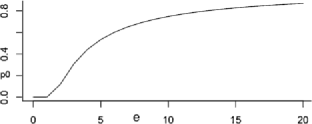
Figure 4: The curve $p_{0}$ vs. $\mathbf{e}_{F}$ where for a graph $F$ with $\mathbf{e}_{F}$ many edges our large deviation result holds when $p>p_{0}$.

The proof of Theorem 14 uses the same arguments that were used in the triangle case. Here, the tilted measure leads to an exponential random graph model where the Hamiltonian depends on number of copies of $F$ in the random graph. Let $\beta\geq 0,h\in\mathbb{R}$ be two fixed numbers. As before, we will identify elements of $\Omega:=\{0,1\}^{n\choose 2}$ with undirected graphs on a set of $n$ vertices. For each $\mathbf{x}\in\Omega$, let $N(\mathbf{x})$ denote the number of copies of $F$ in the graph defined by $\mathbf{x}$, and let $E(\mathbf{x})=\sum_{i<j}x_{ij}$ denote the number of edges. Let $\mathbf{X}=(X_{ij})_{1\leq i<j\leq n}$ be a random element of $\Omega$ following the probability measure proportional to $e^{H(\mathbf{x})}$, where $H$ is the Hamiltonian

$$H(\mathbf{x})=\frac{\beta}{(n-2)_{\mathbf{v}_{F}-2}}N(\mathbf{x})+hE(\mathbf{x}),$$

where $(n)_{m}=\frac{n!}{(n-m)!}$. Recall that $\mathbf{v}_{F}$ is the number of vertices in the graph $F$. The scaling was done to make the two summands comparable. Also we used $(n-2)_{\mathbf{v}_{F}-2}$ instead of $n^{\mathbf{v}_{F}}$ to make calculations simpler. Let $Z_{n}(\beta,h)$ be the partition function. Note that $N(\mathbf{x})$ can be written as

$$N(\mathbf{x})=\frac{1}{\alpha_{F}}\mathop{\sum_{1\leq t_{1},t_{2},\ldots,t_{\mathbf{v}_{F}}\leq n,}}_{t_{i}\neq t_{j}\ \mathrm{for}\ i\neq j}\prod_{(i,j)\in E(F)}x_{t_{i}t_{j}}.$$ (16)

For $\mathbf{x}\in\Omega,1\leq i<j\leq n$, define $\mathbf{x}_{(i,j)}^{1}$ as the element of $\Omega$ which is same as $\mathbf{x}$ in every coordinate except for the $(i,j)$th coordinate where the value is $1$. Similarly, define $\mathbf{x}_{(i,j)}^{0}$. For $i<j$, define the random variable

$$L_{ij}:=\frac{N(\mathbf{X}_{(i,j)}^{1})-N(\mathbf{X}_{(i,j)}^{0})}{(n-2)_{\mathbf{v}_{F}-2}}.$$

The main idea is as in the triangle case. We show that $L_{ij}$’s satisfy a system of “mean-field equations” similar to (8) which has a unique solution under the condition of Theorem 15. In fact, we will show that $L_{ij}$ “$\approx$” $u^{*}$ for all $i<j$ and $E(\mathbf{X})$ “$\approx$” ${n\choose 2}\varphi(u^{*})$ under the condition of Theorem 15. Now note that we can write the Hamiltonian as

$$H(\mathbf{X})=\frac{\beta}{\mathbf{e}_{F}}\sum_{i<j}X_{ij}L_{ij}+h\sum_{i<j}X_{ij},$$

which is approximately equal to $h^{*}E(\mathbf{X})$ where $h^{*}=h+\beta u^{*}/\mathbf{e}_{F}$. Now the remaining is a calculus exercise.

So the first step in proving the large deviation bound is the following theorem, which gives the limiting free energy in the “high temperature” regime. Note the similarity with the triangle case.

Theorem 15

Suppose we have $\beta\geq 0$, $h\in\mathbb{R}$, and $Z_{n}(\beta,h)$ defined as above. Define a function $\varphi\dvtx[0,1]\to\mathbb{R}$ as

$$\varphi(x)=\frac{e^{\beta x+h}}{1+e^{\beta x+h}}.$$

Suppose $\beta$ and $h$ are such that the equation $\alpha_{F}u=2\mathbf{e}_{F}\varphi(u)^{\mathbf{e}_{F}-1}$ has a unique solution $u^{*}$ in $[0,1]$ and $2\mathbf{e}_{F}(\mathbf{e}_{F}-1)\varphi(u^{*})^{\mathbf{e}_{F}-2}\varphi^{\prime}(u^{*})<\alpha_{F}$. Then

$$\lim_{n\to\infty}\frac{\log Z_{n}(\beta,h)}{n^{2}}=-\frac{1}{2}I(\varphi(u^{*}),\varphi(0))-\frac{1}{2}\log\bigl{(}1-\varphi(0)\bigr{)}+\frac{\beta\varphi(u^{*})^{\mathbf{e}_{F}}}{\alpha_{F}},$$

where $I(\cdot,\cdot)$ is the function defined in (4). Moreover, there exists a constant $K(\beta,h)$ that depends only on $\beta$ and $h$ (and not on $n$) such that difference between $n^{-2}\log Z_{n}(\beta,h)$ and the limit is bounded by $K(\beta,h)n^{-1/2}$ for all $n$.

Here also we can identify the region where the conditions in Theorem 15 hold. Let

$$h_{0}=\log(\mathbf{e}_{F}-1)-\frac{\mathbf{e}_{F}}{\mathbf{e}_{F}-1}.$$ (17)

For $h<h_{0}$, there exist exactly two solutions $0<a_{*}=a_{*}(h)<1/2<a^{*}=a^{*}(h)<\infty$ of the equation

$$\log x+\frac{1+x}{(\mathbf{e}_{F}-1)x}+h=0.$$

Define $a_{*}(h)=a^{*}(h)=1/(\mathbf{e}_{F}-1)$ for $h=h_{0}$ and

$$\beta_{*}(h)=\frac{\alpha_{F}(1+a_{*})^{\mathbf{e}_{F}}}{2\mathbf{e}_{F}(\mathbf{e}_{F}-1)a_{*}}\quad\mbox{and}\quad\beta^{*}(h)=\frac{\alpha_{F}(1+a^{*})^{\mathbf{e}_{F}}}{2\mathbf{e}_{F}(\mathbf{e}_{F}-1)a^{*}}$$ (18)

for $h\leq h_{0}$.

Lemma 16

Let $S$ be the set of pairs $(h,\beta)$ for which the function

$$\psi(u):=2\mathbf{e}_{F}\varphi(u)^{\mathbf{e}_{F}-1}-\alpha_{F}u$$

has a unique root $u^{*}$ in $[0,1]$ and $2\mathbf{e}_{F}(\mathbf{e}_{F}-1)\varphi(u^{*})^{\mathbf{e}_{F}-2}\varphi^{\prime}(u^{*})<\alpha_{F}$ where $\varphi(u):=e^{\beta u+h}/(1+e^{\beta u+h}).$ Then we have

$$S^{c}=\{(h,\beta)\dvtx h\leq h_{0}\mbox{ and }\beta_{*}(h)\leq\beta\leq\beta^{*}(h)\},$$

where $h_{0},\beta^{*},\beta_{*}$ are as given in (17), (18). In particular, $(h,\beta)\in S$ if

$$\beta\leq\frac{\alpha_{F}\mathbf{e}_{F}^{\mathbf{e}_{F}-1}}{2(\mathbf{e}_{F}-1)^{\mathbf{e}_{F}}}\quad\mbox{or}\quad h>h_{0}.$$

In fact, Lemma 16 identifies the critical point and the phase transition curve where the model goes from ordered phase to a disordered phase. But the results above does not say what happens at the boundary or in the low temperature regime. However, note that the mean-field equations hold for all values of $\beta$ and $h$.

2.4 Example: Ising model on $\mathbb{Z}^{d}$

Fix any $\beta\geq 0,h\in\mathbb{R}$ and an integer $d\geq 1$. Also fix $n\geq 2$. Let $\mathbb{B}=\{1,2,\ldots,n+1\}^{d}$ be a hypercube with $(n+1)^{d}$ many points in the $d$-dimensional hypercube lattice $\mathbb{Z}^{d}$. Let $\Omega$ be the graph obtained from $\mathbb{B}$ by identifying the opposite boundary points, that is, for $x=(x_{1},x_{2},\ldots,x_{d}),y=(y_{1},y_{2},\ldots,y_{d})\in\mathbb{B}$ we have $x$ is identified with $y$ if $x_{i}-y_{i}\in\{-n,0,n\}$ for all $i$. This identification is known in the literature as periodic boundary condition. Note that $\Omega$ is the $d$-dimensional lattice torus with linear size $n$. We will write $x\sim y$ for $x,y\in\Omega$ if $x,y$ are nearest neighbors in $\Omega$. Also, let us denote by $N_{x}$ the set of nearest neighbors of $x$ in $\Omega$, that is, $N_{x}=\{y\in\Omega\dvtx y\sim x\}$.

Now, consider the Gibbs measure on $\{+1,-1\}^{\Omega}$ given by the following Hamiltonian

$$H(\bolds{\sigma}):=\beta\sum_{x\sim y,x,y\in\Omega}\sigma_{x}\sigma_{y}+h\sum_{x\in\Omega}\sigma_{x},$$

where $\bolds{\sigma}=(\sigma_{x})_{x\in\Omega}$ is a typical element of $\{+1,-1\}^{\Omega}$. So the probability of a configuration $\bolds{\sigma}\in\{+1,-1\}^{\Omega}$ is

$$\mu_{\beta,h}(\{\bolds{\sigma}\}):=Z_{\beta,h}^{-1}\exp(H(\bolds{\sigma}))=Z_{\beta,h}^{-1}\exp\biggl{(}\beta\sum_{x\sim y,x,y\in\Omega}\sigma_{x}\sigma_{y}+h\sum_{x\in\Omega}\sigma_{x}\biggr{)},$$ (19)

where $Z_{\beta,h}=\sum_{\bolds{\sigma}\in\{+1,-1\}^{\Omega}}e^{H(\bolds{\sigma})}$ is the normalizing constant. Here $\sigma_{x}$ is the spin of the magnetic particle at position $x$ in the discrete torus $\Omega$. This is the famous Ising model of ferromagnetism on the box $\mathbb{B}$ with periodic boundary condition at inverse temperature $\beta$ and external field $h$.

The one-dimensional Ising model is probably the first statistical model of ferromagnetism to be proposed or analyzed ising25 . The model exhibits no phase transition in one dimension. But for dimensions two and above the Ising ferromagnet undergoes a transition from an ordered to a disordered phase as $\beta$ crosses a critical value. The two-dimensional Ising model with no external field was first solved by Lars Onsager in a ground breaking paper onsager44 , who also calculated the critical $\beta$ as $\beta_{c}=\sinh^{-1}(1)$. For dimensions three and above the model is yet to be solved, and indeed, very few rigorous results are known.

In this subsection, we present some concentration inequalities for the Ising model that hold for all values of $\beta$. These “temperature-free” relations are analogous to the mean field equations that we obtained for subgraph counts earlier.

The magnetization of the system, as a function of the configuration $\bolds{\sigma}$, is defined as $m(\bolds{\sigma}):=\frac{1}{|\Omega|}\sum_{x\in\Omega}\sigma_{x}$. For each integer $k\in\{1,2,\ldots,2d\}$, define a degree $k$ polynomial function $r_{k}(\bolds{\sigma})$ of a spin configuration $\bolds{\sigma}$ as follows:

$$r_{k}(\bolds{\sigma}):=\biggl{(}\pmatrix{2d\cr k}|\Omega|\biggr{)}^{-1}\sum_{x\in\Omega}\sum_{S\subseteq N_{x},|S|=k}\sigma_{S},$$ (20)

where $\sigma_{S}=\prod_{x\in S}\sigma_{x}$ for any $S\subseteq\Omega$. In particular $r_{k}(\bolds{\sigma})$ is the average of the product of spins of all possible $k$ out of $2d$ neighbors. Note that $r_{1}(\bolds{\sigma})\equiv m(\bolds{\sigma})$. We will show that when $h=0$ and $n$ is large, $m(\bolds{\sigma})$ and $r_{k}(\bolds{\sigma})$’s satisfy the following “mean-field relation” with high probability under the Gibbs measure:

$$\bigl{(}1-\theta_{0}(\beta)\bigr{)}m(\bolds{\sigma})\approx\sum_{k=1}^{d-1}\theta_{k}(\beta)r_{2k+1}(\bolds{\sigma}).$$ (21)

These relations hold for all values of $\beta\geq 0$. Here, $\theta_{k}$’s are explicit rational functions of $\tanh(2\beta)$ for $k=0,1,\ldots,d-1$, defined in (17) below. [Later, we will prove in Proposition 19 that an external magnetic field $h$ will add an extra linear term in the above relation (21).] The following proposition makes this notion precise in terms of finite sample tail bound. It is a simple consequence of Theorem 1.

Theorem 17

Suppose $\bolds{\sigma}$ is drawn from the Gibbs measure $\mu_{\beta,0}$. Then, for any $\beta\geq 0,n\geq 1$ and $t\geq 0$ we have

$$\mathbb{P}\Biggl{(}\sqrt{|\Omega|}\Biggl{|}\bigl{(}1-\theta_{0}(\beta)\bigr{)}m(\bolds{\sigma})-\sum_{k=1}^{d-1}\theta_{k}(\beta)r_{2k+1}(\bolds{\sigma})\Biggr{|}\geq t\Biggr{)}\leq 2\exp\biggl{(}-\frac{t^{2}}{4b(\beta)}\biggr{)},$$

where $m(\bolds{\sigma}):=\frac{1}{|\Omega|}\sum_{x\in\Omega}\sigma_{x}$ is the magnetization, $r_{k}(\bolds{\sigma})$ is as given in (20) and for $k=0,1,\ldots,d-1$

$$\theta_{k}(\beta) = \frac{1}{4^{d}}\pmatrix{2d\cr 2k+1}\sum_{\bolds{\sigma}\in\{-1,+1\}^{2d}}\tanh\Biggl{(}\beta\sum_{i=1}^{2d}\sigma_{i}\Biggr{)}\prod_{j=1}^{2k+1}\sigma_{j}\quad\mbox{and}$$

$$b(\beta) = |1-\theta_{0}(\beta)|+\sum_{k=1}^{d-1}(2k+1)|\theta_{k}(\beta)|.$$

Moreover, we can explicitly write down $\theta_{0}(\beta)$ as

$$\theta_{0}(\beta)=\frac{1}{4^{d-1}}\sum_{k=1}^{d}k\pmatrix{2d\cr d+k}\tanh(2k\beta)$$

and for $d\geq 2$ there exists $\beta_{1}\in(0,\infty)$, depending on $d$, such that $1-\theta_{0}(\beta)>0$ for $\beta<\beta_{1}$ and $1-\theta_{0}(\beta)<0$ for $\beta>\beta_{1}$.

Here, we may remark that for any fixed $k$, $\theta_{k}(\beta/2d)$ converges to the coefficient of $x^{2k+1}$ in the power series expansion of $\tanh(\beta x)$ and $2d\beta_{1}(d)\downarrow 1$ as $d\to\infty$. For small values of $d$, we can explicitly calculate the $\theta_{k}$’s. For instance, in $d=2$,

$$\theta_{0}(\beta)=\tfrac{1}{2}\bigl{(}\tanh(4\beta)+2\tanh(2\beta)\bigr{)},\qquad\theta_{1}(\beta)=\tfrac{1}{2}\bigl{(}\tanh(4\beta)-2\tanh(2\beta)\bigr{)}.$$

For $d=3$,

$$\theta_{0}(\beta) = \tfrac{3}{16}\bigl{(}\tanh(6\beta)+4\tanh(4\beta)+5\tanh(2\beta)\bigr{)},$$

$$\theta_{1}(\beta) = \tfrac{10}{16}\bigl{(}\tanh(6\beta)-3\tanh(2\beta)\bigr{)},$$

$$\theta_{2}(\beta) = \tfrac{3}{16}\bigl{(}\tanh(6\beta)-4\tanh(4\beta)+5\tanh(2\beta)\bigr{)}.$$

For $d=4$,

$$\theta_{0}(\beta) = \tfrac{1}{16}\bigl{(}\tanh(8\beta)+6\tanh(6\beta)+14\tanh(4\beta)+14\tanh(2\beta)\bigr{)},$$

$$\theta_{1}(\beta) = \tfrac{7}{16}\bigl{(}\tanh(8\beta)+2\tanh(6\beta)-2\tanh(4\beta)-6\tanh(2\beta)\bigr{)},$$

$$\theta_{2}(\beta) = \tfrac{7}{16}\bigl{(}\tanh(8\beta)-2\tanh(6\beta)-2\tanh(4\beta)+6\tanh(2\beta)\bigr{)},$$

$$\theta_{3}(\beta) = \tfrac{1}{16}\bigl{(}\tanh(8\beta)-6\tanh(6\beta)+14\tanh(4\beta)-14\tanh(2\beta)\bigr{)}.$$

Corollary 18

For the Ising model on $\Omega$ at inverse temperature $\beta$ with no external magnetic field for all $t\geq 0$ we have:

if $d=1$,

$$\mathbb{P}\bigl{(}|m(\bolds{\sigma})|\geq t\bigr{)}\leq 2\exp\bigl{(}-\tfrac{1}{4}|\Omega|\bigl{(}1-\tanh(2\beta)\bigr{)}t^{2}\bigr{)};$$

if $d=2$,

$$\mathbb{P}\bigl{(}|[(1-u)^{2}-u^{3}]m(\bolds{\sigma})+u^{3}r_{3}(\bolds{\sigma})|\geq t\bigr{)}\leq 2\exp\biggl{(}-\frac{|\Omega|t^{2}}{32}\biggr{)},$$

where $u=\tanh(2\beta)$ and $r_{3}(\bolds{\sigma})=\frac{1}{4|\Omega|}\sum^{*}\sigma_{x}\sigma_{y}\sigma_{z}$ where the sum $\sum^{*}$ is over all $x,y,z\in\Omega$ such that $|x-y|=2,|z-y|=2,|x-z|=2$;

if $d=3$,

$$\mathbb{P}\bigl{(}|g(u)m(\bolds{\sigma})+5u^{3}(1+u^{2})r_{3}(\bolds{\sigma})-3u^{5}r_{5}(\bolds{\sigma})|\geq t\bigr{)}\leq 2\exp(-c|\Omega|t^{2}),$$

where $c$ is an absolute constant, $g(u)=1-3u+4u^{2}-9u^{3}+3u^{4}-3u^{5}$, $u=\tanh(2\beta)$ and $r_{3},r_{5}$ are as defined in (20).

Although we do not yet know the significance of the above relations, it seems somewhat striking that they are not affected by phase transitions. The exponential tail bounds show that many such relations can hold simultaneously. For completeness, we state below the corresponding result for nonzero external field.

Proposition 19

Suppose $\bolds{\sigma}$ is drawn from the Gibbs measure $\mu_{\beta,h}$. Let $r_{k}(\bolds{\sigma})$, $\theta_{k}(\beta)$, $b(\beta)$ be as in proposition (17). Then, for any $\beta\geq 0,h\in\mathbb{R},n\geq 1$ and $t\geq 0$ we have

$$\mathbb{P}\bigl{(}\bigl{|}\bigl{(}1-\theta_{0}(\beta)\bigr{)}m(\bolds{\sigma})-g(\bolds{\sigma})\bigr{|}\geq t\bigr{)}\leq 2\exp\biggl{(}-\frac{|\Omega|t^{2}}{4b(\beta)(1+\tanh|h|)}\biggr{)},$$ (23)

where

$$g(\bolds{\sigma}):=\sum_{k=1}^{d-1}\theta_{k}(\beta)r_{2k+1}(\bolds{\sigma})+\tanh(h)\Biggl{(}1-\sum_{k=0}^{d-1}\theta_{k}(\beta)s_{2k+1}(\bolds{\sigma})\Biggr{)}$$

and

$$s_{k}(\bolds{\sigma}):=\biggl{(}\pmatrix{2d\cr k}|\Omega|\biggr{)}^{-1}\sum_{x\in\Omega}\sum_{S\subseteq N_{x},|S|=k}\sigma_{S\cup\{x\}}$$

is the average of products of spins over all $k$-stars for $k=1,2,\ldots,2d$ and $\Omega$ is the discrete torus in $\mathbb{Z}^{d}$ with $n^{d}$ many points.

3 Proofs

3.1 Proof of Proposition 4

Instead of proving Theorem 2 first, let us see how it is applied to prove the result for the Curie–Weiss model at critical temperature. The proof is simply an elaboration of the sketch given at the end of Section 2.1.

Suppose $\bolds{\sigma}$ is drawn from the Curie–Weiss model at critical temperature. We construct $\bolds{\sigma}^{\prime}$ by taking one step in the heat-bath Glauber dynamics: a coordinate $I$ is chosen uniformly at random, and $\sigma_{I}$ is replace by $\sigma^{\prime}_{I}$ drawn from the conditional distribution of the $I$th coordinate given $\{\sigma_{j}\dvtx j\neq I\}$. Let

$$F(\bolds{\sigma},\bolds{\sigma}^{\prime}):=\sum_{i=1}^{n}(\sigma_{i}-\sigma^{\prime}_{i})=\sigma_{I}-\sigma^{\prime}_{I}.$$

For each $i=1,2,\ldots,n$, define $m_{i}=m_{i}(\bolds{\sigma})=n^{-1}\sum_{j\neq i}\sigma_{j}.$ An easy computaion gives that $\mathbb{E}(\sigma_{i}|\{\sigma_{j},j\neq i\})=\tanh(m_{i})$ for all $i$ and so we have

$$f(\bolds{\sigma}):=\mathbb{E}(F(\bolds{\sigma},\bolds{\sigma}^{\prime})|\bolds{\sigma})=m-\frac{1}{n}\sum_{i=1}^{n}\tanh(m_{i})=\frac{m}{n}+\frac{1}{n}\sum_{i=1}^{n}g(m_{i}),$$

where $g(x):=x-\tanh(x)$. By definition, $m_{i}(\bolds{\sigma})-m(\bolds{\sigma})=\sigma_{i}/n$ and $m_{i}(\bolds{\sigma}^{\prime})-m(\bolds{\sigma})=(\sigma_{i}+\sigma_{I}-\sigma^{\prime}_{I})/n$ for all $i$. Hence, using Taylor’s expansion up to first degree and noting that $|g^{\prime}(x)|=\tanh^{2}(x)\leq x^{2}$ we have

$$|f(\bolds{\sigma})-f(\bolds{\sigma}^{\prime})| \leq \frac{2}{n}|g^{\prime}(m(\bolds{\sigma}))|+\frac{2+5\max_{|x|\leq 1}|g^{\prime\prime}(x)|}{n^{2}}$$

$$\leq \frac{2}{n}m(\bolds{\sigma})^{2}+\frac{6}{n^{2}}.$$

Clearly, $|F(\bolds{\sigma},\bolds{\sigma}^{\prime})|\leq 2$. Thus, we have

$$\Delta(\bolds{\sigma}):=\frac{1}{2}\mathbb{E}[|f(\bolds{\sigma})-f(\bolds{\sigma}^{\prime})|\cdot|F(\bolds{\sigma},\bolds{\sigma}^{\prime})||\bolds{\sigma}]\leq\frac{2}{n}m(\bolds{\sigma})^{2}+\frac{6}{n^{2}}.$$

Now it is easy to verify that $|x|^{3}\leq 5|x-\tanh x|$ for all $|x|\leq 1$. Note that this is the place where we need $\beta=1$. For $\beta\neq 1$, the linear term dominates in $m-\tanh(\beta m)$. Hence, it follows that

$$m(\bolds{\sigma})^{2}\leq 5^{2/3}|m(\bolds{\sigma})-\tanh m(\bolds{\sigma})|^{2/3}\leq 3|f(\bolds{\sigma})|^{2/3}+{3}{n^{-2/3}},$$

where in the last line we used the fact that $|f(\bolds{\sigma})-(m-\tanh m)|\leq 1/n$ and $5^{2/3}<3$. Thus,

$$\Delta(\bolds{\sigma})\leq\frac{6}{n}|f(\bolds{\sigma})|^{2/3}+\frac{12}{n^{5/3}}$$

and using Corollary 3 with $\alpha=2/3,B=6/n$ and $C=12/n^{5/3}$ we have

$$\mathbb{P}(|m-\tanh m|\geq t+n^{-1})\leq\mathbb{P}\bigl{(}|f(\bolds{\sigma})|\geq t\bigr{)}\leq 2e^{-cnt^{4/3}}$$

for all $t\geq 0$ for some constant $c>0$. This clearly implies that

$$\mathbb{P}(|m|\geq t)\leq\mathbb{P}(|m-\tanh m|\geq t^{3}/5)\leq 2e^{-cnt^{4}}$$

for all $t\geq 0$ and for some absolute constant $c>0$. Thus, we are done.

3.2 Proof of Proposition 6

The proof is along the lines of proof of Proposition 4. Suppose $\mathbf{X}$ is drawn from the distribution $\nu_{n}$. We construct $\mathbf{X}^{\prime}$ as follows: a coordinate $I$ is chosen uniformly at random, and $X_{I}$ is replace by $X^{\prime}_{I}$ drawn from the conditional distribution of the $I$th coordinate given $\{X_{j}\dvtx j\neq I\}$. Let

$$F(\mathbf{X},\mathbf{X}^{\prime}):=\sum_{i=1}^{n}(X_{i}-X^{\prime}_{i})=X_{I}-X^{\prime}_{I}.$$

For each $i=1,2,\ldots,n$, define $m_{i}(\mathbf{X})=n^{-1}\sum_{j\neq i}X_{j}.$ An easy computaion gives that $\mathbb{E}(X_{i}|\{X_{j},j\neq i\})=g(m_{i})$ for all $i=1,2,\ldots,n$ where $g(s)=\frac{d}{ds}(\log\int\exp(x^{2}/2n+sx)\,d\rho(x))$ for $s\in\mathbb{R}$. So we have

$$f(\mathbf{X}):=\mathbb{E}(F(\mathbf{X},\mathbf{X}^{\prime})|\mathbf{X})=m(\mathbf{X})-\frac{1}{n}\sum_{i=1}^{n}g(m_{i}(\mathbf{X})).$$

Define the function

$$h(s)=\frac{s^{2}}{2}-\log\int\exp(sx)\,d\rho(x)\qquad\mbox{for }s\in\mathbb{R}.$$ (24)

Clearly, $h$ is an even function. Recall that $k$ is an integer such that $h^{(i)}(0)=0$ for $0\leq i<2k$ and $h^{(2k)}(0)\neq 0$. We have $k\geq 2$ since $h^{\prime\prime}(0)=1-\int x^{2}\,d\rho(x)=0$.

Now using the fact that $\rho([-L,L])=1$ it is easy to see that $|f(\mathbf{X})-h^{\prime}(m(\mathbf{X}))|\leq c/n$ for some constant $c$ depending on $L$ only. In the subsequent calculations, $c$ will always denote a constant depending only on $L$ that may vary from line to line. Similarly, we have

$$|f(\mathbf{X})-f(\mathbf{X}^{\prime})| \leq \frac{|X_{I}-X^{\prime}_{I}|}{n}\biggl{(}|1-g^{\prime}(m(\mathbf{X}))|+\frac{c(1+\sup_{|x|\leq L}|g^{\prime\prime}(x)|)}{n}\biggr{)}$$

$$\leq \frac{2L}{n}|h^{\prime\prime}(m(\mathbf{X}))|+\frac{c}{n^{2}}.$$

Note that $|h^{\prime\prime}(s)|\leq cs^{2k-2}$ for some constant $c$ for all $s\geq 0$. This follows since $\lim_{s\to 0}h^{\prime\prime}(s)/s^{2k-2}$ exists and $h^{\prime\prime}(\cdot)$ is a bounded function. Also $\lim_{s\to 0}|h^{\prime}(s)|/\break|s|^{2k-1}=|h^{(2k)}(0)|\neq 0$ and $|h^{\prime}(s)|>0$ for $s>0$. So we have $|h^{\prime}(s)|\geq c|s|^{2k-1}$ for some constant $c>0$ and all $|s|\leq L$. From the above results, we deduce that

$$|f(\mathbf{X})-f(\mathbf{X}^{\prime})| \leq \frac{c}{n}|(m(\mathbf{X}))|^{2k-2}+\frac{c}{n^{2}}\leq\frac{c}{n}|h^{\prime}(m(\mathbf{X}))|^{({2k-2})/({2k-1})}+\frac{c}{n^{2}}$$

$$\leq \frac{c}{n}|f(\mathbf{X})|^{({2k-2})/({2k-1})}+\frac{c}{n^{2-{1}/{(2k-1)}}}.$$

Now the rest of the proof follows exactly as for the classical Curie–Weiss model.

3.3 Proof of Theorem 7

First, let us state and prove a simple technical lemma.

Lemma 20

Let $x_{1},\ldots,x_{k},y_{1},\ldots,y_{k}$ be real numbers. Then

$$\max_{1\leq i\leq n}\biggl{|}\frac{e^{x_{i}}}{\sum_{j=1}^{k}e^{x_{j}}}-\frac{e^{y_{i}}}{\sum_{j=1}^{k}e^{y_{j}}}\biggr{|}\leq 2\max_{1\leq i\leq n}|x_{i}-y_{i}|$$

and

$$\Biggl{|}\log\sum_{i=1}^{k}e^{x_{i}}-\log\sum_{i=1}^{k}e^{y_{i}}\Biggr{|}\leq\max_{1\leq i\leq k}|x_{i}-y_{i}|.$$

Fix $1\leq i\leq k$. For $t\in[0,1]$, let

$$h(t)=\frac{e^{tx_{i}+(1-t)y_{i}}}{\sum_{j=1}^{k}e^{tx_{j}+(1-t)y_{j}}}.$$

Then

$$h^{\prime}(t)=\biggl{[}(x_{i}-y_{i})-\frac{\sum_{j=1}^{k}(x_{j}-y_{j})e^{tx_{j}+(1-t)y_{j}}}{\sum_{j=1}^{k}e^{tx_{j}+(1-t)y_{j}}}\biggr{]}h(t).$$

This shows that $|h^{\prime}(t)|\leq 2\max_{i}|x_{i}-y_{i}|$ for all $t\in[0,1]$ and completes the proof of the first assertion. The second inequality is proved similarly. Proof of Lemma 10 Fix two numbers $1\leq i<j\leq n$. Given a configuration $\mathbf{X}$, construct another configuration $\mathbf{X}^{\prime}$ as follows. Choose a point $k\in\{1,\ldots,n\}\setminus\{i,j\}$ uniformly at random, and replace the pair $(X_{ik},X_{jk})$ with $(X^{\prime}_{ik},X^{\prime}_{jk})$ drawn from the conditional distribution given the rest of the edges. Let $L_{ij}^{\prime}$ be the revised value of $L_{ij}$. From the form of the Hamiltonian, it is now easy to read off that for $x,y\in\{0,1\}$,

$$\mathbb{P}(X^{\prime}_{ik}=x,X^{\prime}_{jk}=y|\mathbf{X})$$

$$\qquad\propto\exp\biggl{(}\beta xL_{ik}+\beta yL_{jk}+hx+hy-\frac{\beta}{n}xX_{ij}X_{jk}-\frac{\beta}{n}yX_{ij}X_{ik}+\frac{\beta}{n}xyX_{ij}\biggr{)}.$$

An application of Lemma 20 shows that the terms having $\beta/n$ as coefficient can be “ignored” in the sense that for each $x,y\in\{0,1\}$,

$$\biggl{|}\mathbb{P}(X^{\prime}_{ik}=x,X^{\prime}_{jk}=y|\mathbf{X})-\frac{e^{\beta xL_{ik}+\beta yL_{jk}+hx+hy}}{(1+e^{\beta L_{ik}+h})(1+e^{\beta L_{jk}+h})}\biggr{|}\leq\frac{2\beta}{n}.$$

In particular,

$$|\mathbb{E}(X^{\prime}_{ik}X^{\prime}_{jk}|\mathbf{X})-\varphi(L_{ik})\varphi(L_{jk})|\leq\frac{2\beta}{n}.$$ (25)

Now,

$$\mathbb{E}(L_{ij}-L_{ij}^{\prime}|\mathbf{X}) = \frac{1}{n(n-2)}\sum_{k\notin\{i,j\}}\bigl{(}X_{ik}X_{jk}-\mathbb{E}(X^{\prime}_{ik}X^{\prime}_{jk}|\mathbf{X})\bigr{)}$$

$$= \frac{1}{n-2}L_{ij}-\frac{1}{n(n-2)}\sum_{k\notin\{i,j\}}\mathbb{E}(X^{\prime}_{ik}X^{\prime}_{jk}|\mathbf{X}).$$

Let $F(\mathbf{X},\mathbf{X}^{\prime})=(n-2)(L_{ij}-L^{\prime}_{ij})$ and $f(\mathbf{X})=\mathbb{E}(F(\mathbf{X},\mathbf{X}^{\prime})|\mathbf{X})$. Let

$$g(\mathbf{X})=L_{ij}-\frac{1}{n}\sum_{k\notin\{i,j\}}\varphi(L_{ik})\varphi(L_{jk}).$$

From (25) and (3.3), it follows that

$$|f(\mathbf{X})-g(\mathbf{X})|\leq\frac{2\beta}{n}.$$ (27)

Since $X^{\prime}$ has the same distribution as $X$, the same bound holds for $|f(X^{\prime})-g(X^{\prime})|$ as well. Now clearly, $|F(X,X^{\prime})|\leq 1$. Again, $|g(X)-g(X^{\prime})|\leq 2/n$, and therefore

$$|f(X)-f(X^{\prime})|\leq\frac{4(1+\beta)}{n}.$$

Combining everything, and applying Theorem 1 with $B=0$ and $C=2(1+\beta)/n$, we get

$$\mathbb{P}\bigl{(}|f(\mathbf{X})|\geq t\bigr{)}\leq 2\exp\biggl{(}-\frac{nt^{2}}{4(1+\beta)}\biggr{)}$$

for all $t\geq 0$. From (27), it follows that

$$\mathbb{P}\bigl{(}|g(\mathbf{X})|\geq t\bigr{)}\leq\mathbb{P}\bigl{(}|f(\mathbf{X})|\geq t-2\beta/n\bigr{)}\leq 2\exp\biggl{(}-\frac{nt^{2}}{8(1+\beta)}\biggr{)}$$

for all $t\geq 8\beta/n$. This completes the proof of the tail bound. The bound on the mean absolute value is an easy consequence of the tail bound. Proof of Lemma 11 The proof is in two steps. In the first step, we will get an error bound of order $n^{-1/2}\sqrt{\log n}$. In the second step, we will improve it to $n^{-1/2}$. Define

$$\Delta=\max_{1\leq i<j\leq n}\biggl{|}L_{ij}-\frac{1}{n}\sum_{k\notin\{i,j\}}\varphi(L_{ik})\varphi(L_{jk})\biggr{|}.$$

By Lemma 10 and union bound, we have

$$\mathbb{P}(\Delta\geq t)\leq n^{2}\exp\biggl{(}-\frac{nt^{2}}{8(1+\beta)}\biggr{)}$$

for all $t\geq 8\beta/n$. Intuitively, the above equation says that $\Delta$ is of the order of $\sqrt{\log n/n}$, in fact we have $\mathbb{E}(\Delta^{2})=O(\log n/n)$. Clearly, $\varphi$ is an increasing function. Hence, we have

$$\varphi(L_{\min})^{2}-\Delta\leq L_{\min}\leq L_{\max}\leq\varphi(L_{\max})^{2}+\Delta,$$

where $L_{\max}=\max_{1\leq i<j\leq n}L_{ij}$ and $L_{\min}=\min_{1\leq i<j\leq n}L_{ij}$.

Now assume that there exists a unique solution $u^{*}$ of the equation $\varphi(u)^{2}=u$ with $2\varphi(u^{*})\varphi^{\prime}(u^{*})<1$. For ease of notation, define the function $\psi(u)=\varphi(u)^{2}-u$. We have $\psi(0)>0>\psi(1)$, $u^{*}$ is the unique solution to $\psi(u)=0$ and $\psi^{\prime}(u^{*})<0$. It is easy to see that $\psi^{\prime}(u)=0$ has at most three solution [$\psi^{\prime}(u)=2\beta\varphi(u)^{2}(1-\varphi(u))-1$ is a third degree polynomial in $\varphi(u)$ and $\varphi$ is a strictly increasing function].

Hence, there exist positive real numbers $\varepsilon,\delta$ such that $|\psi(u)|>\varepsilon$ if $|u-u^{*}|>\delta$. Note that $\psi(u)>0$ if $u<u^{*}$ and $\psi(u)<0$ is $u>u^{*}$. Decreasing $\varepsilon,\delta$ without loss of generality, we can assume that

$$\inf_{0<|u-u^{*}|\leq\delta}\biggl{[}\frac{u-u^{*}}{-\psi(u)}\biggr{]}=c>0.$$ (28)

This is possible because $\psi^{\prime}(u^{*})<0$. Note that $\psi(L_{\max})\geq-\Delta$ and $\psi(L_{\min})\leq\Delta$. Thus, we have

$$u^{*}-\delta\leq L_{\min}\leq L_{\max}\leq u^{*}+\delta,$$

when $\Delta<\varepsilon$. Using (28), $u^{*}\leq L_{\max}\leq u^{*}+\delta$ implies that $|L_{\max}-u^{*}|\leq c\Delta$ and $u^{*}-\delta\leq L_{\min}\leq u^{*}$ implies that $|L_{\min}-u^{*}|\leq c\Delta$. Thus, when $\Delta<\varepsilon$, we have $|L_{\max}-u^{*}|\leq c{\Delta}$ and $|L_{\min}-u^{*}|\leq c{\Delta}$ and in particular, $|L_{ij}-u^{*}|\leq c{\Delta}$ for all $i<j$. So we can bound the $L^{2}$ distance of $L_{ij}$ from $u^{*}$ by

$$\mathbb{E}(L_{ij}-u^{*})^{2}\leq c^{2}\mathbb{E}(\Delta^{2})+\mathbb{P}(\Delta\geq\varepsilon)\leq K(\beta,h)\frac{\log n}{n}$$

for all $i<j$.

Now let us move to the second step. Recall from (9) that

$$\mathbb{E}\biggl{|}L_{ij}-\frac{1}{n}\sum_{k\notin\{i,j\}}\varphi(L_{ik})\varphi(L_{jk})\biggr{|}\leq\frac{C(1+\beta)^{1/2}}{n^{1/2}}$$ (29)

for all $i<j$. Let $D_{ij}=L_{ij}-u^{*}$. Using Taylor’s expansion around $u^{*}$ up to degree one, we have

$$\varphi(L_{ik})\varphi(L_{jk})-\varphi(u^{*})^{2} = \varphi(u^{*})\bigl{(}\varphi(L_{ik})-\varphi(u^{*})\bigr{)}+\varphi(u^{*})\bigl{(}\varphi(L_{jk})-\varphi(u^{*})\bigr{)}$$

$${}+\bigl{(}\varphi(L_{ik})-\varphi(u^{*})\bigr{)}\bigl{(}\varphi(L_{jk})-\varphi(u^{*})\bigr{)}$$

$$= \varphi(u^{*})\varphi^{\prime}(u^{*})(D_{ik}+D_{jk})+R_{ijk},$$

where $\mathbb{E}(|R_{ijk}|)\leq C\mathbb{E}(D_{ij}^{2})\leq Cn^{-1}\log n$ for some constant $C$ depending only on $\beta,h$. Thus,

$$\mathbb{E}\biggl{|}L_{ij}-\frac{1}{n}\sum_{k\notin\{i,j\}}\varphi(L_{ik})\varphi(L_{jk})-D_{ij}+\frac{\varphi(u^{*})\varphi^{\prime}(u^{*})}{n}\sum_{k\notin\{i,j\}}(D_{ik}+D_{jk})\biggr{|}$$

(30)

$$\qquad\leq\frac{2u^{*}}{n}+\frac{1}{n}\sum_{k\notin\{i,j\}}\mathbb{E}|R_{ijk}|\leq\frac{C\log n}{n}.$$

Here, we used the fact that $u^{*}=\varphi(u^{*})^{2}$. Combining (29) and (3.3), we have

$$\mathbb{E}\biggl{|}D_{ij}-\frac{\varphi(u^{*})\varphi^{\prime}(u^{*})}{n}\sum_{k\notin\{i,j\}}(D_{ik}+D_{jk})\biggr{|}\leq\frac{C}{\sqrt{n}}$$

for all $i<j$. By symmetry, $\mathbb{E}|D_{ij}|$ is the same for all $i,j$. Thus, finally we have

$$\mathbb{E}|L_{ij}-u^{*}|=\mathbb{E}|D_{ij}|\leq\frac{1}{1-2\varphi(u^{*})\varphi^{\prime}(u^{*})}\cdot\frac{C}{\sqrt{n}}=\frac{K(\beta,h)}{\sqrt{n}},$$

where $K(\beta,h)$ is a constant depending on $\beta,h$.

When $\psi(u)=0$ has a unique solution at $u=u^{*}$ with $2\psi(u^{*})\psi^{\prime}(u^{*})=1$, which happens at the critical point $\beta=(3/2)^{3},h=\log 2-3/2$, instead of (28) we have

$$\inf_{0<|u-u^{*}|\leq\delta}\biggl{[}\frac{(u-u^{*})^{3}}{-\psi(u)}\biggr{]}=c>0$$

since $\psi(u^{*})=\psi^{\prime}(u^{*})=\psi^{\prime\prime}(u^{*})=0$ and $\psi^{\prime\prime\prime}(u^{*})<0$. Then using a similar idea as above one can easily show that

$$\mathbb{E}|L_{ij}-u^{*}|\leq K(\beta,h){n^{-1/6}}$$

for some constant $K$ depending on $\beta,h$. This completes the proof of the lemma. The proof becomes lot easier if we have

$$c:=\varphi(1)\cdot\sup_{0\leq x\leq 1}\frac{|\varphi(x)-\varphi(u^{*})|}{|x-u^{*}|}<\frac{1}{2}.$$ (31)

This is because, by the triangle inequality, we have

$$\sum_{i<j}|L_{ij}-u^{*}| \leq \sum_{i<j}\biggl{|}L_{ij}-\frac{1}{n}\sum_{k\notin\{i,j\}}\varphi(L_{ik})\varphi(L_{jk})\biggr{|}$$

$${}+\sum_{i<j}\biggl{(}\frac{1}{n}\sum_{k\notin\{i,j\}}|\varphi(L_{ik})\varphi(L_{jk})-u^{*}|+\frac{2u^{*}}{n}\biggr{)}.$$

Now recall that condition (31) says that $\varphi(1)|\varphi(x)-\varphi(u^{*})|\leq c|x-u^{*}|$ for all $x\in[0,1]$. Moreover, $L_{ij}\in[0,1]$ for all $i,j$, and $u^{*}=\varphi(u^{*})^{2}$. Thus,

$$|\varphi(L_{ik})\varphi(L_{jk})-u^{*}|\leq c|L_{ik}-u^{*}|+c|L_{jk}-u^{*}|.$$

Combining everything, we get

$$\sum_{i<j}|L_{ij}-u^{*}|\leq\frac{\sum_{i<j}|L_{ij}-{1}/{n}\sum_{k\notin\{i,j\}}\varphi(L_{ik})\varphi(L_{jk})|+nu^{*}}{1-2c}.$$

Taking expectation on both sides, and applying Lemma 10, we get

$$\sum_{i<j}\mathbb{E}|L_{ij}-u^{*}|\leq\frac{C(1+\beta)n^{3/2}}{1-2c}.$$

And this gives the required result. In fact, using basic calculus results one can easily check that condition (31) is satisfied when $h\geq 0$ or $\beta\leq 2$.

Now, we will prove that in the exponential random graph model, the number of edges and number of triangles also satisfy certain “mean-field” relations.

Lemma 21

Recall that $E(\mathbf{x})$ and $T(\mathbf{x})$ denote the number of edges and number of triangles in the graph defined by the edge configuration $\mathbf{x}\in\Omega$. If $\mathbf{X}$ is drawn from the Gibbs’ measure in Theorem 8, we have the bound

$$\mathbb{E}\biggl{|}E(\mathbf{X})-\sum_{i<j}\varphi(L_{ij})\biggr{|} \leq C(1+\beta)^{1/2}n,$$

$$\mathbb{E}\biggl{|}\frac{T(\mathbf{X})}{n}-\frac{1}{3}\sum_{i<j}L_{ij}\varphi(L_{ij})\biggr{|} \leq C(1+\beta)^{1/2}n,$$

where and $C$ is a universal constant.

It is not difficult to see that

$$\mathbb{E}\bigl{(}X_{ij}|(X_{kl})_{(k,l)\neq(i,j)}\bigr{)}=\varphi(L_{ij}).$$

Let us create $\mathbf{X}^{\prime}$ by choosing $1\leq i<j\leq n$ uniformly at random and replacing $X_{ij}$ with $X_{ij}^{\prime}$ drawn from the conditional distribution of $X_{ij}$ given $(X_{kl})_{(k,l)\neq(i,j)}$. Let $F(\mathbf{X},\mathbf{X}^{\prime})={n\choose 2}(X_{ij}-X^{\prime}_{ij})$. Then

$$f(\mathbf{X})=\mathbb{E}(F(\mathbf{X},\mathbf{X}^{\prime})|\mathbf{X})=\sum_{k<l}\bigl{(}X_{kl}-\varphi(L_{kl})\bigr{)}=E(\mathbf{X})-\sum_{k<l}\varphi(L_{kl}).$$

Now $|F(\mathbf{X},\mathbf{X}^{\prime})|\leq{n\choose 2}$ and $|f(\mathbf{X})-f(\mathbf{X}^{\prime})|\leq 1+\beta$. Here we used the fact that $|\varphi^{\prime}(x)|\leq\beta/4$. Combining the above result and Theorem 1 with $B=0,C=\frac{1}{2}(1+\beta){n\choose 2}$, we get the required bound.

Similarly, if we define $F(\mathbf{X},\mathbf{X}^{\prime})={n\choose 2}(X_{ij}L_{ij}-X_{ij}^{\prime}L_{ij})$. Then

$$f(\mathbf{X}) = \mathbb{E}(F(\mathbf{X},\mathbf{X}^{\prime})|\mathbf{X})=\sum_{k<l}\bigl{(}X_{kl}L_{kl}-\varphi(L_{kl})L_{kl}\bigr{)}$$

$$= \frac{3}{n}T(\mathbf{X})-\sum_{k<l}\varphi(L_{kl})L_{kl}.$$

Again, $|F(\mathbf{X},\mathbf{X}^{\prime})|\leq{n\choose 2}$ and $|f(\mathbf{X})-f(\mathbf{X}^{\prime})|\leq C(1+\beta)$. The bound follows easily as before.

The following result is an easy corollary of Lemmas 11 and 21.

Corollary 22

Suppose the conditions of Theorem 8 are satisfied. Then we have

$$\mathbb{E}\biggl{|}E(\mathbf{X})-\frac{n^{2}\varphi(u^{*})}{2}\biggr{|}\leq Cn^{3/2}\quad\mbox{and}\quad\mathbb{E}\biggl{|}\frac{T(\mathbf{X})}{n}-\frac{n^{2}\varphi(u^{*})^{3}}{6}\biggr{|}\leq Cn^{3/2},$$

where $C$ is a constant depending only on $\beta,h$.

Lemma 23

Suppose the conditions of Theorem 8 are satisfied. Let $T_{n}$ be the number of triangles in the Erdős–Rényi graph $G(n,\varphi(0))$. Then there is a constant $K(\beta,h)$ depending only on $\beta$ and $h$ such that for all $n$

$$\biggl{|}\frac{\log\mathbb{P}(|T_{n}-{n\choose 3}\varphi(u^{*})^{3}|\leq K(\beta,h)n^{5/2})}{n^{2}}-\frac{-I(\varphi(u^{*}),\varphi(0))}{2}\biggr{|}\leq\frac{K(\beta,h)}{\sqrt{n}}.$$

Let $X$ be drawn from the Gibbs’ measure in Theorem 8 with parameters $\beta,h$. From Corollary 22, we see that there exists a constant $K(\beta,h)$ such that (for all $n$)

$$\mathbb{P}\biggl{(}\biggl{|}E(X)-\frac{n^{2}\varphi(u^{*})}{2}\biggr{|}\leq K(\beta,h)n^{3/2}\biggr{)}\geq\frac{3}{4}$$

and

$$\mathbb{P}\biggl{(}\biggl{|}\frac{T(X)}{n}-\frac{n^{2}\varphi(u^{*})^{3}}{6}\biggr{|}\leq K(\beta,h)n^{3/2}\biggr{)}\geq\frac{3}{4}.$$

Now let

$$A=\biggl{\{}x\in\{0,1\}^{n}\dvtx\biggl{|}\frac{T(x)}{n}-\frac{n^{2}\varphi(u^{*})^{3}}{6}\biggr{|}\leq K(\beta,h)n^{3/2}\biggr{\}}$$

and

$$B=A\cap\biggl{\{}x\in\{0,1\}^{n}\dvtx\biggl{|}E(x)-\frac{n^{2}\varphi(u^{*})}{2}\biggr{|}\leq K(\beta,h)n^{3/2}\biggr{\}}.$$

Now suppose $Y=(Y_{ij})_{1\leq i<j\leq n}$ is a collection of i.i.d. random variables satisfying $\mathbb{P}(Y_{ij}=1)=1-\mathbb{P}(Y_{ij}=0)=\varphi(0)$ and $Z=(Z_{ij})_{1\leq i<j\leq n}$ is another collection of i.i.d. random variables with $\mathbb{P}(Z_{ij}=1)=1-\mathbb{P}(Z_{ij}=0)=\varphi(u^{*})$. Without loss of generality, we can assume that $K(\beta,h)$ was chosen large enough to ensure that (again, for all $n$) $\mathbb{P}(Z\in A)\geq 1/2$ and $\mathbb{P}(Z\in B)\geq 1/2$. Now, it follows directly from the definition of $A$ and Lemma 20 that

$$\biggl{|}\log\sum_{x\in A}e^{hE(x)}-\log\sum_{x\in A}e^{{\beta T(x)}/{n}+hE(x)}+\frac{\beta n^{2}\varphi(u^{*})^{3}}{6}\biggr{|}$$

$$\qquad=\biggl{|}\log\sum_{x\in A}e^{hE(x)+{\beta n^{2}\varphi(u^{*})^{3}}/{6}}-\log\sum_{x\in A}e^{{\beta T(x)}/{n}+hE(x)}\biggr{|}$$

$$\qquad\leq\beta\max_{x\in A}\biggl{|}\frac{T(x)}{n}-\frac{n^{2}\varphi(u^{*})^{3}}{6}\biggr{|}\leq\beta K(\beta,h)n^{3/2}.$$

Next, observe that

$$\biggl{|}\log\sum_{x\in A}e^{{\beta T(x)}/{n}+hE(x)}-\log\sum_{x\in\Omega}e^{{\beta T(x)}/{n}+hE(x)}\biggr{|}$$

(34)

$$\qquad=|{\log}\mathbb{P}(X\in A)|\leq|{\log}(3/4)|.$$

Similarly, we have

$$\biggl{|}\log\sum_{x\in B}e^{{\beta T(x)}/{n}+hE(x)}-\log\sum_{x\in\Omega}e^{{\beta T(x)}/{n}+hE(x)}\biggr{|}$$

(35)

$$\qquad=|{\log}\mathbb{P}(X\in B)|\leq|{\log}(1/2)|,$$

where we used the fact that $\mathbb{P}(X\in A\cap C)\geq\mathbb{P}(X\in A)+\mathbb{P}(X\in C)-1$. Combining the last two inequalities, we get

$$\biggl{|}\log\sum_{x\in A}e^{{\beta T(x)}/{n}+hE(x)}-\log\sum_{x\in B}e^{{\beta T(x)}/{n}+hE(x)}\biggr{|}\leq\log(8/3).$$ (36)

Next, note that by the definition of $B$ and Lemma 20, we have that for any $h^{\prime}$,

$$\hskip 20.0pt\biggl{|}\log\sum_{x\in B}e^{{\beta T(x)}/{n}+hE(x)}-\frac{n^{2}(h-h^{\prime})\varphi(u^{*})}{2}-\frac{\beta n^{2}\varphi(u^{*})^{3}}{6}-\log\sum_{x\in B}e^{h^{\prime}E(x)}\biggr{|}$$

$$\hskip 20.0pt\qquad\leq\sup_{x\in B}\biggl{|}\frac{\beta T(x)}{n}+hE(x)-\frac{n^{2}(h-h^{\prime})\varphi(u^{*})}{2}-\frac{\beta n^{2}\varphi(u^{*})^{3}}{6}-h^{\prime}E(x)\biggr{|}$$ (37)

$$\hskip 20.0pt\qquad\leq(\beta+|h-h^{\prime}|)K(\beta,h)n^{3/2}.$$

Now, choose $h^{\prime}=\log\frac{\varphi(u^{*})}{1-\varphi(u^{*})}$. Then

$$\biggl{|}\log\sum_{x\in B}e^{h^{\prime}E(x)}-\log\sum_{x\in\Omega}e^{h^{\prime}E(x)}\biggr{|}=|{\log\mathbb{P}}(Z\in B)|\leq\log 2.$$ (38)

Adding up (3.3), (36), (3.3) and (38), and using the triangle inequality, we get

$$\quad\biggl{|}\log\sum_{x\in A}e^{hE(x)}-\frac{n^{2}(h-h^{\prime})\varphi(u^{*})}{2}-\log\sum_{x\in\Omega}e^{h^{\prime}E(x)}\biggr{|}\leq K^{\prime}(\beta,h)n^{3/2},$$ (39)

where $K^{\prime}(\beta,h)$ is a constant depending only on $\beta,h$. For any $s\in\mathbb{R}$, a trivial verification shows that

$$\log\sum_{x\in\Omega}e^{sE(x)}=\pmatrix{n\cr 2}\log(1+e^{s}).$$

Again, note that $\log\mathbb{P}(Y\in A)=\log\sum_{x\in A}e^{hE(x)}-\log\sum_{x\in\Omega}e^{hE(x)}$. Therefore, it follows from inequality (39) that

$$\biggl{|}\frac{\log\mathbb{P}(Y\in A)}{n^{2}}-\frac{(h-h^{\prime})\varphi(u^{*})+\log(1+e^{h^{\prime}})-\log(1+e^{h})}{2}\biggr{|}\leq\frac{K^{\prime}(\beta,h)}{\sqrt{n}}.$$

Now $h=\log\frac{\varphi(0)}{1-\varphi(0)}$ and $h^{\prime}=\log\frac{\varphi(u^{*})}{1-\varphi(u^{*})}$. Also, $\log(1+e^{h})=-\log(1-\varphi(0))$ and $\log(1+e^{h^{\prime}})=-\log(1-\varphi(u^{*}))$. Substituting these in the above expression, we get

$$\biggl{|}\frac{\log\mathbb{P}(Y\in A)}{n^{2}}-\frac{-I(\varphi(u^{*}),\varphi(0))}{2}\biggr{|}\leq\frac{K^{\prime}(\beta,h)}{\sqrt{n}}.$$

This completes the proof of the lemma.

We are now ready to finish the proof of Theorem 8. Proof of Theorem 8 Note that by adding the terms in (3.3), (3.3) and (38) from the proof of Lemma 23, and applying the triangle inequality, we get

$$\biggl{|}\frac{\log Z_{n}(\beta,h)}{n^{2}}-\frac{(h-h^{\prime})\varphi(u)}{2}-\frac{\beta\varphi(u)^{3}}{6}-\frac{1}{2}\log(1+e^{h^{\prime}})\biggr{|}\leq\frac{K(\beta,h)}{\sqrt{n}}.$$

This can be rewritten as

$$\biggl{|}\frac{\log Z_{n}(\beta,h)}{n^{2}}+\frac{I(\varphi(u),\varphi(0))+\log(1-\varphi(0))}{2}-\frac{\beta\varphi(u)^{3}}{6}\biggr{|}\leq\frac{K(\beta,h)}{\sqrt{n}}.$$

This completes the proof of Theorem 8.

Note that the proof of Theorem 8 contains a proof for the lower bound in the general case. We provide the proof below for completeness.

Proof of Lemma 9 Fix any $r\in(0,1)$. Define the set $B_{r}$ as

$$B_{r}=\biggl{\{}x\in\{0,1\}^{n}\dvtx\biggl{|}\frac{T(x)}{n}-\frac{n^{2}r^{3}}{6}\biggr{|}\leq K(r)n^{3/2},\biggl{|}E(x)-\frac{n^{2}r}{2}\biggr{|}\leq K(r)n^{3/2}\biggr{\}},$$

where $K(r)$ is chosen in such a way that $\mathbb{P}(Z\in B_{r})\geq 1/2$ where $Z=((Z_{ij}))_{i<j}$ and $Z_{ij}$’s are i.i.d. Bernoulli$(r)$. From the proof of Lemma 23, it is easy to see that

$$\biggl{|}\log\sum_{x\in B_{r}}e^{{\beta T(x)}/{n}+hE(x)}-\frac{n^{2}}{2}\biggl{(}(h-h^{\prime})r+\frac{\beta r^{3}}{3}+\log(1+e^{h^{\prime}})\biggr{)}\biggr{|}\leq K^{\prime}n^{3/2},$$

where $h^{\prime}=\log\frac{r}{1-r}$ and $K^{\prime}$ is a constant depending on $\beta,h,r$. Simplifying, we have

$$\frac{2}{n^{2}}\log Z_{n}(\beta,h) \geq \frac{2}{n^{2}}\log\sum_{x\in B_{r}}e^{{\beta T(x)}/{n}+hE(x)}$$

$$\geq \frac{\beta r^{3}}{3}+\log(1-p)-I(r,p)-\frac{K^{\prime}}{\sqrt{n}}$$

for all $r$ where $p=e^{h}/(1+e^{h})$. Now taking limit as $n\to\infty$ and maximizing over $r$ we have the first inequality (9). Given $\beta,h$, define the function

$$f(r)=\frac{\beta r^{3}}{3}+\log(1-p)-I(r,p),$$

where $p=e^{h}/(1+e^{h})$. One can easily check that $f^{\prime}(r)\gtreqqless 0$ iff $\varphi(u)^{2}-u\gtreqqless 0$ for $u=r^{2}$. From this fact, the second equality follows.

Lemma 24

Let $T_{n}$ be the number of triangles in the Erdős–Rényi graph $G(n,\varphi(0))$. Then there is a constant $K(\beta,h)$ depending only on $\beta$ and $h$ such that for all $n$

$$\frac{\log\mathbb{P}(T_{n}\geq{n\choose 3}\varphi(u^{*})^{3})}{n^{2}}\leq\frac{-I(\varphi(u^{*}),\varphi(0))}{2}+\frac{K(\beta,h)}{\sqrt{n}}.$$

By Markov’s inequality, we have

$$\frac{\log\mathbb{P}(T_{n}\geq{n\choose 3}\varphi(u^{*})^{3})}{n^{2}}\leq-\frac{\beta}{n^{3}}\pmatrix{n\cr 3}\varphi(u^{*})^{3}+\frac{\mathbb{E}(e^{\beta T_{n}/n})}{n^{2}}.$$

From the last part of Theorem 8, it is easy to obtain an optimal upper bound of the second term on the right-hand side, which finishes the proof of the lemma. Proof of Theorem 7 Given $p$ and $r$, if for all $r^{\prime}$ belonging to a small neighborhood of $r$ there exist $\beta$ and $h$ satisfying the conditions of Theorem 8 such that $\varphi(0)=p$ and $\varphi(u^{*})=r^{\prime}$, then a combination of Lemma 23 and Lemma 24 implies the conclusion of Theorem 7. If $p\geq p_{0}=2/(2+e^{3/2})$, we can just choose $h\geq h_{0}=-\log 2-3/2$ such that $p=e^{h}/(1+e^{h})$ and conclude, from Theorem 8, Lemma 23 and Lemma 12, that the large deviations limit holds for any $\beta\geq 0$. Varying $\beta$ between $0$ and $\infty$, it is possible to get for any $r\geq p$ a $\beta$ such that $\varphi(u^{*})=r$.

For $p\leq p_{0}$, we again choose $h$ such that $\varphi(0)=p$. Note that $h\leq h_{0}$. The large deviations limit should hold for any $r\geq p$ for which there exists $\beta>0$ such that $r=\varphi(u^{*})=\sqrt{u^{*}}$ and $(h,\beta)\in S$. It is not difficult to verify that given $h$, $u^{*}$ is a continuously increasing function of $\beta$ in the regime for which $(h,\beta)\in S$. Recall the settings of Lemma 12. Thus, the values of $r$ that is allowed is in the set $(p,p_{*})\cup(p^{*},1]$, where $p^{*},p_{*}$ are the unique nontouching solutions to the equations

$$\sqrt{p^{*}}=\frac{e^{\beta_{*}(h)p^{*}+h}}{1+e^{\beta_{*}(h)p^{*}+h}},\qquad\sqrt{p_{*}}=\frac{e^{\beta^{*}(h)p_{*}+h}}{1+e^{\beta^{*}(h)p_{*}+h}}.$$

This completes the proof of Theorem 7.

Finally, let us round up by proving Lemma 12. Proof of Lemma 12 Fix $h\in\mathbb{R}$. Define the function

$$\psi(x;h,\beta):=\varphi(x;h,\beta)^{2}-x,$$

where

$$\varphi(x;h,\beta)=\frac{e^{\beta x+h}}{1+e^{\beta x+h}}\qquad\mbox{for }x\in[0,1].$$

For simplicity, we will omit $\beta,h$ in $\varphi(x;\beta,h)$ and $\psi(x;\beta,h)$ when there is no chance of confusion. Note that $\psi(0)>0>\psi(1)$. Hence, the equation $\varphi(x;\beta,h)=0$ has at least one solution. Also we have $\psi^{\prime}(x)=2\beta\varphi(x)^{2}(1-\varphi(x))-1$ and $\varphi$ is strictly increasing. Hence, the equation $\psi^{\prime}(x)=0$ has at most three solutions. So either the function $\psi$ is strictly decreasing or there exist two numbers $0<a<b<1$ such that $\psi$ is strictly decreasing in $[0,a]\cup[b,1]$ and strictly increasing in $[a,b]$. From the above observations, it is easy to see that the equation $\psi(x)=0$ has at most three solutions for any $\beta,h$. If $\psi(x)=0$ has exactly two solutions, then $\psi^{\prime}=0$ at one of the solution.

Let $u_{*}=u_{*}(h,\beta)$ and $u^{*}=u^{*}(h,\beta)$ be the smallest and largest solutions of $\psi(x;h,\beta)=0$, respectively. If $u_{*}=u^{*}$, we have a unique solution of $\psi(x)=0$. From the fact that $\frac{\partial}{\partial\beta}\psi(x;h,\beta)>0$ for all $x\in[0,1],\beta\geq 0,h\in\mathbb{R}$, we can deduce that given $h$, $u_{*}(h,\beta)$ and $u^{*}(h,\beta)$ are increasing functions of $\beta$. Note that $u_{*}$ is left continuous and $u^{*}$ is right continuous in $\beta$ given $h$. Also note that given $h\in\mathbb{R}$, $u^{*}=u_{*}$ if $\beta>0$ is very small or very large. So, we can define $\beta_{*}(h)$ and $\beta^{*}(h)$ such that for $\beta<\beta_{*}(h)$ and for $\beta>\beta^{*}(h)$ we have $u_{*}(h,\beta)=u^{*}(h,\beta)$. $\beta_{*}$ is the largest and $\beta^{*}$ is the smallest such number.

Therefore, we can deduce that at $\beta=\beta_{*}(h),\beta^{*}(h)$ the equation $\psi(x;h,\beta)=0$ has exactly two solutions. Thus, we have two real numbers $x_{*},x^{*}\in[0,1]$ such that

$$\varphi(x)^{2}=x\quad\mbox{and}\quad 2\beta\varphi(x)^{2}\bigl{(}1-\varphi(x)\bigr{)}=1$$

for $(x,\beta)=(x_{*},\beta_{*})$ or $(x^{*},\beta^{*})$. Thus, we have $2\beta x(1-\sqrt{x})=1$ and

$$h=\log\frac{\sqrt{x}}{1-\sqrt{x}}-\frac{1}{2(1-\sqrt{x})}$$

for $x=x_{*},x^{*}$. Define $a_{*}=x_{*}^{-1/2}-1$ and $a^{*}=(x^{*})^{-1/2}-1$. Note that $x=(1+a)^{-2},\beta=(1+a)^{3}/2a^{2}$ for $(x,a,\beta)=(x_{*},a_{*},\beta_{*})$ or $(x^{*},a^{*},\beta^{*})$ and we have

$$h=-\log a-\frac{1+a}{2a}$$ (41)

for $a=a_{*},a^{*}$. Now the function $g(x)=-\log x-({1+x})/{2x}$ is strictly increasing for $x\in(0,1/2]$ and strictly decreasing for $x\geq 1/2$. So (41) has no solution for $h\geq g(1/2)=\log 2-3/2=:h_{0}$. For $h<h_{0}$, equation (41) has exactly two solutions and for $h=h_{0}$ equation (41) has one solution. One can easily check that $\beta_{*}\leq\beta^{*}$ implies that $a_{*}\leq a^{*}$. Also from the fact that (41) has at most two solutions, we have that for $\beta\in(\beta_{*},\beta^{*})$ the equation $\psi(u)=0$ has exactly three solutions.

3.4 Proof of Lemma 13

For simplicity, we will prove the result only for the lower boundary part, that is, for $(h,\beta)=\gamma(t)$ with $t<1/2$. The proof for the upper boundary is similar. Fix $t<1/2$. Let us briefly recall the setup. The function $\psi(u)=\varphi(u)^{2}-u$ has two roots at $0<u^{*}<v^{*}<1$ and $\psi^{\prime}(u_{*})<0$ while $\psi^{\prime}(v^{*})=0,\psi^{\prime\prime}(v^{*})<0$. See Figure 5 for the graph of the function $\psi$ when $t=1/4$.

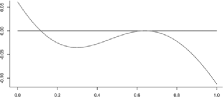
Figure 5: The function $\psi(\cdot)$ for $(h,\beta)=\gamma(1/4)$.

Define the function

$$f(r)=\frac{\beta r^{3}}{3}+\log(1-p)-I(r,p)\qquad\mbox{for }r\in(0,1).$$

From the proof of Lemma 9 and the fact that $\psi^{\prime}(u)<0$ for $u\in(u^{*},v^{*})$, it is easy to see that $f(\varphi(u^{*}))>f(\varphi(v^{*}))$ and

$$\frac{2}{n^{2}}\log Z_{n}(\beta,h)\geq f(\varphi(u^{*}))-\frac{K}{\sqrt{n}},$$ (42)

where $K$ depends on $\beta,h$. Now, using the same idea used in the proof of Lemma 11, we have

$$\mathbb{P}(\Delta\geq t)\leq n^{2}\exp\biggl{(}-\frac{nt^{2}}{8(1+\beta)}\biggr{)}$$

for all $t\geq 8\beta/n$ and $\psi(L_{\max})\geq-\Delta,\psi(L_{\min})\leq\Delta$ where

$$\Delta=\max_{1\leq i<j\leq n}\biggl{|}L_{ij}-\frac{1}{n}\sum_{k\notin\{i,j\}}\varphi(L_{ik})\varphi(L_{jk})\biggr{|}.$$

Hence, there exists $\varepsilon_{0}>0,c>0$ such that whenever $\Delta<\varepsilon_{0}$ we have $L_{\min}\geq u^{*}-c\Delta$ and either $L_{\max}\leq u^{*}+c\Delta$ or $|L_{\max}-v^{*}|\leq c\sqrt{\Delta}$. Define

$$U=\{L_{\max}<(u^{*}+v^{*})/2\}.$$ (43)

Then again using the idea used in Lemma 11 one can easily show that

$$\mathbb{E}(\mathbh{1}_{U}\cdot|L_{ij}-u^{*}|)\leq\frac{K(\beta,h)}{n^{1/2}}\qquad\mbox{for all }i<j.$$

We will show that $\mathbb{P}(U^{c})\leq(\log n)^{2}/n$ and it will imply that

$$\mathbb{E}(|L_{ij}-u^{*}|)\leq\mathbb{E}(\mathbh{1}_{U}\cdot|L_{ij}-u^{*}|)+\mathbb{P}(U^{c})\leq\frac{K(\beta,h)}{n^{1/2}}\qquad\mbox{for all }i<j.$$

Then the rest of the assertions follow using the steps in the proof of Theorem 23.

Hence, let us concentrate on the event $U^{c}$. It is enough to restrict to the event $U^{c}\cap\{|L_{\max}-v^{*}|\leq c\sqrt{\Delta}\}\cap\{L_{\min}\geq u^{*}-c\Delta\}$. Here, the rough idea is that, a large fraction of $L_{ij}$’s has to be near $v^{*}$ in order to make $L_{\max}\simeq v^{*}$. Suppose $L_{\max}=L_{i_{0}j_{0}}$. Define the set

$$A=\{k\dvtx L_{i_{0}k}<L_{\max}-\delta_{1}\},$$

where $\delta_{1}$ will be chosen later such that $\delta_{1}+c\sqrt{\Delta}<v^{*}-u^{*}$. Note that $\varphi(u)^{2}\leq\max\{u,u^{*}\}$ for all $u$ and by assumption $|L_{\max}-v^{*}|\leq c\sqrt{\Delta}$. Thus, $\varphi(L_{ij})\leq\sqrt{L_{\max}}$ for all $i,j$ and $\varphi(L_{i_{0}k})\leq\sqrt{L_{\max}-\delta_{1}}\leq\sqrt{L_{\max}}(1-\delta_{1}/2)$ for $k\in A$. Thus, we have

$$L_{\max}=L_{i_{0}j_{0}}\leq\Delta+\frac{1}{n}\sum_{k\neq i_{0},j_{0}}\varphi(L_{i_{0}k})\varphi(L_{j_{0}k})\leq\Delta+L_{\max}-\frac{|A|\delta_{1}}{2n},$$

which clearly implies that $\frac{|A|}{n}\leq\frac{2\Delta}{\delta_{1}}.$ Similarly, define the set $A_{j}=\{k\dvtx L_{jk}<L_{\max}-\delta_{2}\}$ where $\delta_{2}$ will be chosen later such that $\delta_{2}+c\sqrt{\Delta}<v^{*}-u^{*}$. Using the same idea as before, for $j\notin A$ we have

$$L_{\max}-\delta_{1}\leq L_{i_{0}j}\leq\Delta+L_{\max}-\frac{|A_{j}|\delta_{2}}{2n}\quad\mbox{or}\quad\frac{|A_{j}|}{n}\leq\frac{2(\Delta+\delta_{1})}{\delta_{2}}:=M\qquad(\mbox{say}).$$

Choose $\delta_{2}=\Delta^{1/5},\delta_{1}=\Delta^{3/5}$. Then we have

$$\sum_{i<j}|L_{ij}-L_{\max}|^{2} \leq \frac{n|A|+nM+n^{2}\delta_{2}^{2}}{2}$$

$$\leq \frac{n^{2}\Delta}{\delta_{1}}+\frac{n^{2}(\Delta+\delta_{1})}{\delta_{2}}+\frac{n^{2}\delta_{2}^{2}}{2}$$

$$\leq 4n^{2}\Delta^{2/5}.$$

Thus, by symmetry and Hölder’s inequality, we have

$$\mathbb{E}(\mathbh{1}_{U^{c}}\cdot|L_{ij}-v^{*}|^{2}) \leq K\mathbb{E}(\mathbh{1}_{U^{c}}\cdot\Delta^{2/5})\leq K\mathbb{P}(U^{c})^{9/10}\cdot\mathbb{E}(\Delta^{4})^{1/10}$$

$$\leq \frac{K(\log n)^{1/5}}{n^{1/5}}\mathbb{P}(U^{c})^{9/10}$$

for some constant $K$. Now using Lemma 21 and (3.4) we have

$$\mathbb{E}\biggl{[}\biggl{|}E(\mathbf{X})-\frac{n^{2}\varphi(v^{*})}{2}\biggr{|}\Big{|}U^{c}\biggr{]} \leq \frac{Cn^{9/5}(\log n)^{1/5}}{\mathbb{P}(U^{c})^{1/10}}\quad\mbox{and}$$

$$\mathbb{E}\biggl{[}\biggl{|}\frac{T(\mathbf{X})}{n}-\frac{n^{2}\varphi(v^{*})^{3}}{6}\biggr{|}\Big{|}U^{c}\biggr{]} \leq \frac{Cn^{9/5}(\log n)^{1/5}}{\mathbb{P}(U^{c})^{1/10}}.$$

If $\mathbb{P}(U^{c})>(\log n)^{2}/n$, from inequality (3.4) we have

$$\mathbb{P}\biggl{(}\biggl{|}E(\mathbf{X})-\frac{n^{2}\varphi(v^{*})}{2}\biggr{|}\geq Kn^{19/10}\big{|}U^{c}\biggr{)}\leq\frac{1}{4}$$

and

$$\mathbb{P}\biggl{(}\biggl{|}\frac{T(\mathbf{X})}{n}-\frac{n^{2}\varphi(v^{*})^{3}}{6}\biggr{|}\geq Kn^{19/10}\big{|}U^{c}\biggr{)}\leq\frac{1}{4}$$

for some large constant $K$ depending on $\beta,h$. Now define the set

$$B=\biggl{\{}x\in\{0,1\}^{n}\dvtx\biggl{|}\frac{T(x)}{n}-\frac{n^{2}\varphi(v^{*})^{3}}{6}\biggr{|}\leq Kn^{19/10},\biggl{|}E(x)-\frac{n^{2}\varphi(v^{*})}{2}\biggr{|}\leq Kn^{19/10}\biggr{\}}.$$

Using the same idea used in the proof of Lemma 23, one can again show that

$$\biggl{|}\frac{2}{n^{2}}\log(Z_{n}\mathbb{P}(U^{c}))-f(\varphi(v^{*}))\biggr{|}\leq\frac{K}{n^{1/10}}$$

for some constant $K$ depending on $\beta,h$. The crucial fact is that $\mathbb{P}(\{L_{\max}(\mathbf{Z})>(u^{*}+v^{*})/2\}\cap\{\mathbf{Z}\in B\})$ is bounded away from zero when $\mathbf{Z}=((Z_{ij}))_{i<j}\sim$ G$(n,\varphi(v^{*}))$. Thus, we have

$$\biggl{|}\frac{2}{n^{2}}\log Z_{n}-f(\varphi(v^{*}))\biggr{|}\leq\frac{K}{n^{1/10}}.$$

But this leads to a contradiction, since by (42) we have

$$\frac{2}{n^{2}}\log Z_{n}(\beta,h)\geq f(\varphi(u^{*}))-\frac{K}{\sqrt{n}}$$

and $f(\varphi(u^{*}))>f(\varphi(v^{*}))$. Thus, we have $\mathbb{P}(U^{c})\leq(\log n)^{2}/n$ and we are done.

3.5 Proof of Theorem 15

The proof is almost an exact copy of the proof of Theorem 8. Recall the definition of $L_{ij}$,

$$L_{ij}:=\frac{N(\mathbf{X}_{(i,j)}^{1})-N(\mathbf{X}_{(i,j)}^{0})}{(n-2)_{\mathbf{v}_{F}-2}}\qquad\mbox{for }i<j.$$ (46)

In fact, we can write $L_{ij}$ explicitly as a horrible sum

$$L_{ij}=\frac{1}{\alpha_{F}(n-2)_{\mathbf{v}_{F}-2}}\mathop{\sum_{t_{1}<t_{2}<\cdots<t_{\mathbf{v}_{F}-2}}}_{t_{l}\in[n]\setminus\{i,j\}\ \mathrm{for}\ \mathrm{all}\ l}\sum_{(a,b)\in E(F)}{\sum_{\pi}}^{\prime}\mathop{\prod_{(k,l)\in E(F)}}_{(k,l)\neq(a,b)}X_{\pi_{k}\pi_{l}},$$

where the sum $\sum^{\prime}$ is over all one-one onto map $\pi$ from $V(F)=[\mathbf{v}_{F}]$ to $\{a,b,t_{1},\ldots,t_{\mathbf{v}_{F}-2}\}$ where $\{\pi(a),\pi(b)\}=\{i,j\}$. Now, we briefly state the main steps. First, we have $\mathbb{E}(X_{ij}|\mbox{rest})=\varphi(L_{ij})$. Moreover, using Lemma 20 it is easy to see that $|\mathbb{E}(\prod_{j=1}^{k}X_{i_{2j-1}i_{2j}}|\mbox{rest})-\prod_{j=1}^{k}\varphi(L_{i_{2j-1}i_{2j}})|\leq C\beta/n$ for every distinct pairs $(i_{1},i_{2}),\ldots,(i_{2k-1},i_{2k})$ where $C$ is an universal constant.

Now, fix $1\leq i<j\leq n$. Given a configuration $\mathbf{X}$, construct another one $\mathbf{X}^{\prime}$ in the following way. Choose $\mathbf{v}_{F}-2$ distinct points uniformly at random without replacement from $[n]\setminus\{i,j\}$. Replace the coordinates in $\mathbf{X}$ corresponding to the edges in the complete subgraph formed by the chosen points including $i,j$ (except that we do not change $X_{ij}$) by values drawn from the conditional distribution given the rest of the edges. Call the new configuration $\mathbf{X}^{\prime}$. Define the antisymmetric function $F(\mathbf{X},\mathbf{X}^{\prime}):=(n-2)_{\mathbf{v}_{F}-2}(L_{ij}-L^{\prime}_{ij}).$ and $f(\mathbf{X}):=\mathbb{E}(F(\mathbf{X},\mathbf{X}^{\prime})|\mathbf{X})$. Using the same idea as before and Theorem 1, we have

$$\mathbb{P}(|L_{ij}-g_{ij}|\geq t)\leq\exp\bigl{(}-cnt^{2}/(1+\beta)\bigr{)},$$ (47)

where $c$ is an absolute constant and $g_{ij}$ is obtained from $L_{ij}$ by replacing $X_{kl}$ by $\varphi(L_{kl})$ for all $k<l$. Note that there is a slight difference with the calculation in the triangle case, since we have to consider collections of edges where some are modified and some are not. But their contribution will be of the order of $n^{-1}$. Also the conditions on $\varphi$ arises in the following way, if all the $L_{ij}$’s are constant, say equal to $u$, then from the “mean-field equations” for $L_{ij}$’s we must have

$$u \approx \frac{1}{\alpha_{F}(n-2)_{\mathbf{v}_{F}-2}}\mathop{\sum_{t_{1}<t_{2}<\cdots<t_{\mathbf{v}_{F}-2}}}_{t_{l}\in[n]\setminus\{i,j\}\ \mathrm{for}\ \mathrm{all}\ l}\sum_{(a,b)\in E(F)}{\sum_{\pi}}^{\prime}\varphi(u)^{\mathbf{e}_{F}-1}$$

$$= \frac{2\mathbf{e}_{F}}{\alpha_{F}}\varphi(u)^{\mathbf{e}_{F}-1}.$$

The next step is to show that under the conditions on $\varphi$, we have $\mathbb{E}|L_{ij}-u^{*}|\leq Kn^{-1/2}$ for all $i<j$ where $K=K(\beta,h)$ is a constant depending only on $\beta,h$. The crucial fact is that the behavior of the function $\varphi(u)^{k}-au$ where $a>0$ is a positive constant and $k\geq 2$ is a fixed integer, is same as the behavior of the function $\varphi(u)^{2}-u$.

Now it will follow (using the same proof used for Lemma 21) that

$$\mathbb{E}\biggl{|}E(\mathbf{X})-\frac{n^{2}\varphi(u^{*})}{2}\biggr{|}\leq Cn^{3/2}$$

and

$$\mathbb{E}\biggl{|}N(\mathbf{X})-\frac{(n)_{\mathbf{v}_{F}}\varphi(u^{*})^{\mathbf{e}_{F}}}{\alpha_{F}}\biggr{|}\leq Cn^{\mathbf{v}_{F}-1/2},$$

where $C$ is a constant depending only on $\beta,h$. The rest of the proof follows using the arguments used in the proof of Theorem 8.

Proof of Theorem 14 Using the method of proof for the triangle case and the result from Theorem 15, the proof follows easily.

Proof of Lemma 16 The proof is same as the proof of Lemma 12 except for the constants.

3.6 Proof of Theorem 17

Suppose $\bolds{\sigma}$ is drawn from the Gibbs distribution $\mu_{\beta,h}$. We construct $\bolds{\sigma}^{\prime}$ by taking one step in the heat-bath Glauber dynamics as follows: choose a position $I$ uniformly at random from $\Omega$, and replace the $I$th coordinate of $\bolds{\sigma}$ by an element drawn from the conditional distribution of the $\sigma_{I}$ given the rest. It is easy to see that $(\bolds{\sigma},\bolds{\sigma}^{\prime})$ is an exchangeable pair. Let

$$F(\bolds{\sigma},\bolds{\sigma}^{\prime}):=|\Omega|\bigl{(}m(\bolds{\sigma})-m(\bolds{\sigma}^{\prime})\bigr{)}=\sigma_{I}-\sigma^{\prime}_{I}$$

be an antisymmetric function in $\bolds{\sigma},\bolds{\sigma}^{\prime}$. Since the Hamiltonian is a simple explicit function, one can easily calculate the conditional distribution of the spin of the particle at position $x$ given the spins of the rest. In fact, we have $\mathbb{E}(\sigma_{x}|\{\sigma_{y},y\neq x\}])=\tanh(2\beta dm_{x}(\bolds{\sigma}))$ where $m_{x}(\bolds{\sigma}):=\frac{1}{2d}\sum_{y\in N_{x}}\sigma_{y}$ is the average spin of the neighbors of $x$ for $x\in\Omega$. Now, using Fourier–Walsh expansion we can write the function $\tanh(2\beta dm_{x}(\bolds{\sigma}))$ as sums of products of spins in the following way. We have

$$\tanh(2d\beta m_{x}(\bolds{\sigma}))=\sum_{k=0}^{2d}a_{k}(\beta)\sum_{|S|=k,S\subseteq N_{x}}\sigma_{S},$$ (48)

where

$$a_{k}(\beta):=\frac{1}{2^{2d}}\sum_{\bolds{\sigma}\in\{-1,+1\}^{2d}}\tanh\Biggl{(}\beta\sum_{i=1}^{2d}\sigma_{i}\Biggr{)}\prod_{j=1}^{k}\sigma_{j}$$ (49)

for $k=0,1,\ldots,2d$. It is easy to see that $a_{k}(\beta)=0$ if $k$ is even and $a_{k}(\beta)$ is a rational function of $\tanh(2\beta)$ if $k$ is odd. Note that the dependence of $a_{k}$ on $d$ is not stated explicitly. Thus, using (48) and the definitions in (20) we have

$$f(\bolds{\sigma}) = \mathbb{E}[F(\bolds{\sigma},\bolds{\sigma}^{\prime})|\bolds{\sigma}]=\frac{1}{|\Omega|}\sum_{x\in\Omega}E[\sigma_{x}-\sigma^{\prime}_{x}|\bolds{\sigma}]$$

$$= m(\bolds{\sigma})-\frac{1}{|\Omega|}\sum_{x\in\Omega}\tanh(2\beta dm_{x}(\bolds{\sigma}))$$

$$= \bigl{(}1-2da_{1}(\beta)\bigr{)}m(\bolds{\sigma})-\sum_{k=1}^{d-1}\pmatrix{2d\cr 2k+1}a_{2k+1}(\beta)r_{2k+1}(\bolds{\sigma}).$$

Define $\theta_{k}(\beta):={2d\choose 2k+1}a_{2k+1}(\beta)$ for $k=0,1,\ldots,d-1$. Note that we can explicitly calculate the value of $\theta_{0}(\beta)$ as follows:

$$\theta_{0}(\beta)=\frac{1}{4^{d}}\sum_{\bolds{\sigma}\in\{-1,+1\}^{2d}}\tanh\Biggl{(}\beta\sum_{i=1}^{2d}\sigma_{i}\Biggr{)}\sum_{i=1}^{2d}\sigma_{i}=\frac{2}{4^{d}}\sum_{k=1}^{d}2k\pmatrix{2d\cr d+k}\tanh(2k\beta).$$

Now, we have $|F(\bolds{\sigma},\bolds{\sigma}^{\prime})|\leq 2$ and

$$|f(\bolds{\sigma})-f(\bolds{\sigma}^{\prime})|\leq\frac{2}{|\Omega|}\Biggl{(}|1-\theta_{0}(\beta)|+\sum_{k=1}^{d-1}(2k+1)\theta_{k}(\beta)\Biggr{)}=\frac{2}{|\Omega|}b(\beta)$$

for all values of $\bolds{\sigma},\bolds{\sigma}^{\prime}$. Hence, the condition of Theorem 1 is satisfied with $B=0$, $C=2|\Omega|^{-1}b(\beta)$. So by part (ii) of Theorem 1, we have

$$\mathbb{P}\Biggl{(}\sqrt{|\Omega|}|\bigl{(}1-\theta_{0}(\beta)\bigr{)}m(\bolds{\sigma})-\sum_{k=1}^{d-1}\theta_{k}(\beta)r_{2k+1}(\bolds{\sigma})|\geq t\Biggr{)}\leq 2\exp\biggl{(}-\frac{t^{2}}{4b(\beta)}\biggr{)}$$

for all $t>0$. Obviously, $\theta_{0}(\cdot)$ is a strictly increasing function of $\beta$. Also, we have $\theta_{0}(0)=0$ and

$$\theta_{0}(\infty):=\lim_{\beta\to\infty}\theta_{0}(\beta)=\frac{1}{4^{d-1}}\sum_{k=1}^{d}k\pmatrix{2d\cr d+k}.$$

For $d=1$, we have $\theta_{0}(\infty)=1$ and for $d\geq 2$ we have

$$\theta_{0}(\infty) \geq \frac{1}{4^{d-1}}\Biggl{[}2\sum_{k=1}^{d}\pmatrix{2d\cr d+k}-\pmatrix{2d\cr d+1}\Biggr{]}$$

$$= \frac{1}{4^{d-1}}\biggl{[}2^{2d}-\pmatrix{2d\cr d}-\pmatrix{2d\cr d+1}\biggr{]}$$

$$= 4-\frac{8}{2^{2d+1}}\pmatrix{2d+1\cr d+1}$$

and from the fact that $\sum_{k=d-1}^{d+2}{2d+1\choose k}\leq 2^{2d+1}$ we have

$$\frac{1}{2^{2d+1}}\pmatrix{2d+1\cr d+1}\leq\frac{d+2}{4(d+1)}\leq\frac{1}{3}\qquad\mbox{for }d\geq 2.$$

Hence, for $d\geq 2$ we have $\theta_{0}(\infty)>1$ and there exists $\beta_{1}\in(0,\infty)$, depending on $d$, such that $1-\theta_{0}(\beta)>0$ for $\beta<\beta_{1}$ and $1-\theta_{0}(\beta)<0$ for $\beta>\beta_{1}$. This completes the proof.

3.7 Proof of Proposition 19

The proof is almost same as the proof of Proposition 17. Define $\bolds{\sigma},\bolds{\sigma}^{\prime}$ as before. Define the antisymmetric function $F(\bolds{\sigma},\bolds{\sigma}^{\prime})$ as follows:

$$F(\bolds{\sigma},\bolds{\sigma}^{\prime}):\! = |\Omega|\bigl{(}1+\tanh(h)\tanh(2\beta dm_{I}(\bolds{\sigma}))\bigr{)}\bigl{(}m(\bolds{\sigma})-m(\bolds{\sigma}^{\prime})\bigr{)}$$

$$= \bigl{(}1+\tanh(h)\tanh(2\beta dm_{I}(\bolds{\sigma}))\bigr{)}(\sigma_{I}-\sigma^{\prime}_{I}).$$

Recall that $m_{x}(\bolds{\sigma}):=\frac{1}{2d}\sum_{y\in N_{x}}\sigma_{y}$ is the average spin of the neighbors of $x$ for $x\in\Omega$. Now under $\mu_{\beta,h}$, we have

$$\mathbb{E}(\sigma_{x}|\{\sigma_{y},y\neq x\}) = \tanh\bigl{(}2\beta dm_{x}(\bolds{\sigma})+h\bigr{)}$$

$$= \frac{\tanh(h)+\tanh(2\beta dm_{x}(\bolds{\sigma}))}{1+\tanh(h)\tanh(2\beta dm_{x}(\bolds{\sigma}))}.$$

Thus, we have

$$f(\bolds{\sigma}) = \mathbb{E}(F(\bolds{\sigma},\bolds{\sigma}^{\prime})|\bolds{\sigma})$$

$$= \frac{1}{|\Omega|}\sum_{x\in\Omega}\bigl{(}1+\tanh(h)\tanh(2\beta dm_{x}(\bolds{\sigma}))\bigr{)}\mathbb{E}(\sigma_{x}-\sigma^{\prime}_{x}|\bolds{\sigma})$$

$$= m(\bolds{\sigma})-\tanh(h)+\frac{1}{|\Omega|}\sum_{x\in\Omega}\bigl{(}\tanh(h)\sigma_{x}-1\bigr{)}\tanh(2\beta dm_{x}(\bolds{\sigma})).$$

After some simplifications and using the definitions of the functions, $r,s$ we have

$$f(\bolds{\sigma}) = \bigl{(}1-\theta_{0}(\beta)\bigr{)}m(\bolds{\sigma})-\sum_{k=1}^{d-1}\theta_{k}(\beta)r_{2k+1}(\bolds{\sigma})$$

$${}-\tanh(h)\Biggl{(}1-\sum_{k=0}^{d-1}\theta_{k}(\beta)s_{2k+1}(\bolds{\sigma})\Biggr{)}.$$

Now for all values of $\bolds{\sigma},\bolds{\sigma}^{\prime}$ we have

$$|f(\bolds{\sigma})-f(\bolds{\sigma}^{\prime})|\leq\frac{2}{|\Omega|}b(\beta)(1+\tanh|h|)$$

and the proof henceforth is exactly as in the proof of Proposition 17.

3.8 Proof of Theorem 2

Assume that $\psi(0)>0$. We will handle the case $\psi(0)=0$ later. Note that condition (1) implies that $x^{\alpha}/\psi(x)$ is a nondecreasing function for $x>0$. Define the function

$$\varphi(x):=\frac{x^{2}}{\psi(x)}\quad\mbox{and}\quad\gamma(x):=2-\frac{x\psi^{\prime}(x)}{\psi(x)}\qquad\mbox{for }x\neq 0$$

and $\varphi(0)=0,\gamma(0)=2$. Clearly, we have $2-\alpha\leq\gamma(x)\leq 2$ for all $x\in\mathbb{R}$. Now, $\limsup_{x\to 0}\varphi(x)\leq\lim_{x\to 0+}x^{2-\alpha}/\psi(1)=0=\varphi(0)$ as $\alpha<2$. Also $\varphi(x)$ is differentiable in $\mathbb{R}\setminus\{0\}$ with

$$\varphi^{\prime}(x)=\frac{x\gamma(x)}{\psi(x)}>0\qquad\mbox{for }x\neq 0.$$ (50)

Hence, $\varphi$ is absolutely continuous in $\mathbb{R}$ and is increasing for $x\geq 0$.

Define $Y=f(X)$. First, we will prove that all moments of $\varphi(Y)$ are finite. Next, we will estimate the moments which will in turn show that $\varphi(Y)^{1/2}$ has finite exponential moment in $\mathbb{R}$. Finally, using Chebyshev’s inequality we will prove the tail probability.

By monotonicity of $\psi$ in $[0,\infty)$ and definition of $\alpha$, we have

$$0\leq\frac{x\psi^{\prime}(x)}{\psi(x)}\leq\alpha\qquad\mbox{for all }x\geq 0.$$ (51)

It also follows from (50) that $0\leq(\log\varphi(x))^{\prime}\leq 2/x$ for $x>0$ and integrating we have $\varphi(x)\leq\varphi(1)x^{2}$ for all $x\geq 1$. Hence, $\varphi(x)=\varphi(|x|)\leq\varphi(1)(1+x^{2})$ for all $x\in\mathbb{R}$ and this, combined with our assumption that $\mathbb{E}(|f(X)|^{k})<\infty$ for all $k\geq 1$, implies that $\mathbb{E}(\varphi(Y)^{k})<\infty\mbox{ for all }k\geq 1.$

Define

$$\beta:=\biggl{\lceil}\frac{5(2-\alpha)+\delta+1/4}{(2-\alpha)^{2}}\biggr{\rceil}\geq 3.$$

Fix an integer $k\geq\beta$ and define

$$g(x)=\frac{x^{2k-1}}{\psi^{k}(x)}\quad\mbox{and}\quad h(x)=\frac{x^{2k-2}}{\psi^{k}(x)}\qquad\mbox{for }x\in\mathbb{R}.$$

Clearly, $\mathbb{E}(|Yg(Y)|)<\infty$. Note that $g,h$ are continuously differentiable in $\mathbb{R}$ as $k\geq 3$. Moreover, for $x\in\mathbb{R}$ we have, $|g^{\prime}(x)|=h(x)|k\gamma(x)-1|\leq(2k-1)h(x)$, $h^{\prime}(x)=(k\gamma(x)-2){x^{2k-3}}/{\psi^{k}(x)}$ and

$$h^{\prime\prime}(x)=\bigl{[}\bigl{(}k\gamma(x)-2\bigr{)}\bigl{(}k\gamma(x)-3\bigr{)}+kx\gamma^{\prime}(x)\bigr{]}\frac{x^{2k-4}}{\psi^{k}(x)}.$$

We also have

$$x\gamma^{\prime}(x)=-\frac{x\psi^{\prime}(x)}{\psi(x)}\biggl{(}1-\frac{x\psi^{\prime}(x)}{\psi(x)}\biggr{)}-\frac{x\psi^{\prime\prime}(x)}{\psi(x)}\geq-1/4-\delta$$

for $x\in\mathbb{R}$. Now $k\geq\beta$ implies that

$$\bigl{(}k\gamma(x)-2\bigr{)}\bigl{(}k\gamma(x)-3\bigr{)}+kx\gamma^{\prime}(x)$$

$$\qquad\geq\bigl{(}k(2-\alpha)-2\bigr{)}\bigl{(}k(2-\alpha)-3\bigr{)}-k(\delta+1/4)\geq 0$$

for all $x$. Thus, $h^{\prime\prime}(x)\geq 0$ for all $x$ and $h$ is convex in $\mathbb{R}$.

Let $X^{\prime},F(X,X^{\prime})$ be as given in the hypothesis. Define $Y^{\prime}=f(X^{\prime})$. Recall that $(X,X^{\prime})$ is an exchangeable pair and so is $(Y,Y^{\prime})$. Using the fact that $f(X)=\mathbb{E}(F(X,X^{\prime})|X)$ almost surely, exchangeability of $(X,X^{\prime})$ and antisymmetry of $F$, we have

$$\mathbb{E}(Yg(Y)) = \mathbb{E}(f(X)g(Y))=\mathbb{E}(F(X,X^{\prime})g(Y))$$

$$= \tfrac{1}{2}\mathbb{E}\bigl{(}F(X,X^{\prime})\bigl{(}g(Y)-g(Y^{\prime})\bigr{)}\bigr{)}.$$

Now, for any $x<y$ we have

$$\biggl{|}\frac{g(x)-g(y)}{x-y}\biggr{|}=\biggl{|}\int_{0}^{1}g^{\prime}\bigl{(}tx+(1-t)y\bigr{)}\,dt\biggr{|}\leq(2k-1)\int_{0}^{1}h\bigl{(}tx+(1-t)y\bigr{)}\,dt$$

and convexity of $h$ implies that

$$\int_{0}^{1}h\bigl{(}tx+(1-t)y\bigr{)}\,dt\leq\int_{0}^{1}\bigl{(}th(x)+(1-t)h(y)\bigr{)}\,dt=\bigl{(}h(x)+h(y)\bigr{)}/2.$$

Hence, from (3.8), we have

$$\mathbb{E}(Yg(Y)) \leq \frac{2k-1}{4}\mathbb{E}\bigl{(}|(Y-Y^{\prime})F(X,X^{\prime})|\bigl{(}h(Y)+h(Y^{\prime})\bigr{)}\bigr{)}$$

$$= (2k-1)\mathbb{E}(\Delta(X)h(Y))\leq(2k-1)\mathbb{E}(\psi(Y)h(Y)),$$

where the equality follows by definition of $\Delta(X)$ and exchangeability of $(Y,Y^{\prime})$. Thus, for any $k\geq\beta$ we have, from (3.8),

$$\mathbb{E}(\varphi(Y)^{k})\leq(2k-1)\mathbb{E}(\varphi(Y)^{k-1}).$$ (54)

Using induction for $k\geq\beta$, we have

$$\mathbb{E}(\varphi(Y)^{k})\leq\frac{(2k)!2^{\beta}\beta!}{2^{k}k!(2\beta)!}\mathbb{E}(\varphi(Y)^{\beta})\qquad\mbox{for }k\geq\beta.$$

Also Hölder’s inequality applied to (54) for $k=\beta$ implies that $\mathbb{E}(\varphi(Y)^{\beta})\leq(2\beta-1)^{\beta}$. Thus, we have

$$\mathbb{E}(\varphi(Y)^{k})\leq\cases{\dfrac{(2k)!2^{\beta}\beta!}{k!2^{k}(2\beta)!}\mathbb{E}(\varphi(Y)^{\beta}),&\quad if $k>\beta$,\vspace*{2pt}\cr(2\beta-1)^{k},&\quad if $0\leq k\leq\beta$.}$$ (55)

Note that we have $e^{x}\leq e^{x}+e^{-x}=2\sum_{k\geq 0}x^{2k}/(2k)!$ for all $x\in\mathbb{R}$. Combining everything, we finally have

$$\mathbb{E}(\exp(\theta\varphi(Y)^{1/2})) \leq 2\sum_{k=0}^{\infty}\frac{\theta^{2k}}{(2k)!}\mathbb{E}(\varphi(Y)^{k})$$

$$\leq \frac{2^{\beta+1}\beta!}{(2\beta)!}\mathbb{E}(\varphi(Y)^{\beta})\sum_{k=\beta}^{\infty}\frac{\theta^{2k}}{2^{k}k!}+\sum_{k=0}^{\beta-1}\frac{2(2\beta-1)^{k}\theta^{2k}}{(2k)!}$$

$$\leq C_{\beta}\exp(\theta^{2}/2)$$

for all $\theta\geq 0$ where the constant $C_{\beta}$ is given by

$$C_{\beta}:=\max\biggl{\{}\frac{2(2\beta-1)^{k}2^{k}k!}{(2k)!}\Big{|}0\leq k\leq\beta\biggr{\}}.$$

Here, we used the fact that $(2k)!\geq 2^{2k-1}k!^{2}/k$. Now recall that $\varphi$ is an increasing function in $[0,\infty)$. Thus, using Chebyshev’s inequality for $\exp(\theta\varphi(x)^{1/2})$ with $\theta=\varphi(t)^{1/2}$ we have

$$\mathbb{P}\bigl{(}|f(X)|\geq t\bigr{)}\leq C_{\beta}e^{-\theta\varphi(t)^{1/2}+\theta^{2}/2}=C_{\beta}e^{-\varphi(t)/2}.$$

Now suppose that $\psi(0)=0$. For $\varepsilon>0$ fixed, define $\psi_{\varepsilon}(x)=\psi(x)+\varepsilon$. Clearly, we have $\Delta(X)\leq\psi_{\varepsilon}(f(X))$ a.s. and $\psi_{\varepsilon}$ satisfies all the other properties of $\psi$ including

$$x\psi^{\prime}_{\varepsilon}(x)/\psi_{\varepsilon}(x)=x\psi^{\prime}(x)/\psi(x)\cdot{\psi(x)}/{\bigl{(}\psi(x)+\varepsilon\bigr{)}}\leq\alpha$$

and

$$x\psi^{\prime\prime}_{\varepsilon}(x)/\psi_{\varepsilon}(x)=x\psi^{\prime\prime}(x)/\psi(x)\cdot{\psi(x)}/{\bigl{(}\psi(x)+\varepsilon\bigr{)}}\leq\delta$$

for all $x>0$. Hence, all the above results hold for $\psi_{\varepsilon}$ and $\varphi_{\varepsilon}(x)=x^{2}/\psi_{\varepsilon}(x)$. Now $\varphi_{\varepsilon}\uparrow\varphi$ as $\varepsilon\downarrow 0$. Letting $\varepsilon\downarrow 0$, we have the result.

When $\psi$ is once differentiable with $\alpha<2$, it is easy to see that the function $h$ is nondecreasing (need not be convex) in $[0,\infty)$ for $k\geq\beta:=\lceil 2/(2-\alpha)\rceil$. In that case, we have

$$\int_{0}^{1}h\bigl{(}tx+(1-t)y\bigr{)}\,dy\leq\max_{z\in[x,y]}h(z)\leq h(x)+h(y)$$

for $x\leq y$. Hence, we have the recursion

$$\mathbb{E}(\varphi(Y)^{k})\leq 2(2k-1)\mathbb{E}(\varphi(Y)^{k-1})$$ (56)

for $k\geq\beta$. Using the same proof as before, it then follows that

$$\mathbb{P}\bigl{(}|f(X)|\geq t\bigr{)}\leq Ce^{-\varphi(t)/4},$$

where $C$ depends only on $\alpha$.

References

- (1) {barticle}[mr] \bauthor\bsnmBarthe, \bfnmF.\binitsF., \bauthor\bsnmCattiaux, \bfnmP.\binitsP. and \bauthor\bsnmRoberto, \bfnmC.\binitsC. (\byear2005). \btitleConcentration for independent random variables with heavy tails. \bjournalAMRX Appl. Math. Res. Express \bvolume2 \bpages39–60. \bidmr=2173316 \endbibitem
- (2) {barticle}[vtex] \bauthor\bsnmBarthe, \bfnmFranck\binitsF., \bauthor\bsnmCattiaux, \bfnmPatrick\binitsP. and \bauthor\bsnmRoberto, \bfnmCyril\binitsC. (\byear2006). \btitleInterpolated inequalities between exponential and Gaussian, Orlicz hypercontractivity and isoperimetry. \bjournalRev. Mat. Iberoamericana \bvolume22 \bpages993–1067. \bidmr=2320410 \endbibitem
- (3) {bincollection}[vtex] \bauthor\bsnmBhamidi, \bfnmS.\binitsS., \bauthor\bsnmBresler, \bfnmG.\binitsG. and \bauthor\bsnmSly, \bfnmA.\binitsA. (\byear2008). \btitleMixing time of exponential random graphs. In \bbooktitleProc. of the 49th Annual IEEE Symp. on FOCS \bpages803–812. \bpublisherIEEE Computer Society, \baddressWashington, DC. \endbibitem
- (4) {barticle}[mr] \bauthor\bsnmBobkov, \bfnmSergey G.\binitsS. G. (\byear2007). \btitleLarge deviations and isoperimetry over convex probability measures with heavy tails. \bjournalElectron. J. Probab. \bvolume12 \bpages1072–1100 (electronic). \bidmr=2336600 \endbibitem
- (5) {barticle}[vtex] \bauthor\bsnmBobkov, \bfnmS. G.\binitsS. G. and \bauthor\bsnmLedoux, \bfnmM.\binitsM. (\byear2000). \btitleFrom Brunn–Minkowski to Brascamp–Lieb and to logarithmic Sobolev inequalities. \bjournalGeom. Funct. Anal. \bvolume10 \bpages1028–1052. \biddoi=10.1007/PL00001645, mr=1800062 \endbibitem
- (6) {bbook}[mr] \bauthor\bsnmBollobás, \bfnmBéla\binitsB. (\byear2001). \btitleRandom Graphs, \bedition2nd ed. \bseriesCambridge Studies in Advanced Mathematics \bvolume73. \bpublisherCambridge Univ. Press, \baddressCambridge. \bidmr=1864966 \endbibitem
- (7) {barticle}[mr] \bauthor\bsnmBolthausen, \bfnmE.\binitsE. (\byear1987). \btitleLaplace approximations for sums of independent random vectors. II. Degenerate maxima and manifolds of maxima. \bjournalProbab. Theory Related Fields \bvolume76 \bpages167–206. \biddoi=10.1007/BF00319983, mr=906774 \endbibitem
- (8) {bmisc}[vtex] \bauthor\bsnmBolthausen, \bfnmE.\binitsE., \bauthor\bsnmComets, \bfnmF.\binitsF. and \bauthor\bsnmDembo, \bfnmA.\binitsA. (\byear2009). \bhowpublishedLarge deviations for random matrices and random graphs. Unpublished manuscript. \endbibitem
- (9) {barticle}[mr] \bauthor\bsnmBoucheron, \bfnmStéphane\binitsS., \bauthor\bsnmLugosi, \bfnmGábor\binitsG. and \bauthor\bsnmMassart, \bfnmPascal\binitsP. (\byear2003). \btitleConcentration inequalities using the entropy method. \bjournalAnn. Probab. \bvolume31 \bpages1583–1614. \biddoi=10.1214/aop/1055425791, mr=1989444 \endbibitem
- (10) {bmisc}[vtex] \bauthor\bsnmChatterjee, \bfnmSourav\binitsS. (\byear2005). \btitleConcentration inequalities with exchangeable pairs. \bnotePh.D. thesis, Stanford Univ. Available at arXiv:math/0507526. \bidmr=2622431 \endbibitem
- (11) {barticle}[mr] \bauthor\bsnmChatterjee, \bfnmSourav\binitsS. (\byear2007). \btitleStein’s method for concentration inequalities. \bjournalProbab. Theory Related Fields \bvolume138 \bpages305–321. \biddoi=10.1007/s00440-006-0029-y, mr=2288072 \endbibitem
- (12) {barticle}[mr] \bauthor\bsnmChatterjee, \bfnmSourav\binitsS. (\byear2007). \btitleConcentration of Haar measures, with an application to random matrices. \bjournalJ. Funct. Anal. \bvolume245 \bpages379–389. \biddoi=10.1016/j.jfa.2007.01.003, mr=2309833 \endbibitem
- (13) {bmisc}[vtex] \bauthor\bsnmChatterjee, \bfnmS.\binitsS. and \bauthor\bsnmShao, \bfnmQ.-M.\binitsQ.-M. (\byear2009). \bhowpublishedStein’s method of exchangeable pairs with application to the Curie–Weiss model. Preprint. Available at arXiv:0907.4450. \endbibitem
- (14) {barticle}[mr] \bauthor\bsnmChazottes, \bfnmJ. R.\binitsJ. R., \bauthor\bsnmCollet, \bfnmP.\binitsP., \bauthor\bsnmKülske, \bfnmC.\binitsC. and \bauthor\bsnmRedig, \bfnmF.\binitsF. (\byear2007). \btitleConcentration inequalities for random fields via coupling. \bjournalProbab. Theory Related Fields \bvolume137 \bpages201–225. \biddoi=10.1007/s00440-006-0026-1, mr=2278456 \endbibitem
- (15) {barticle}[mr] \bauthor\bsnmDöring, \bfnmHanna\binitsH. and \bauthor\bsnmEichelsbacher, \bfnmPeter\binitsP. (\byear2009). \btitleModerate deviations in a random graph and for the spectrum of Bernoulli random matrices. \bjournalElectron. J. Probab. \bvolume14 \bpages2636–2656. \bidmr=2570014 \endbibitem
- (16) {bmisc}[vtex] \bauthor\bsnmEichelsbacher, \bfnmP.\binitsP. and \bauthor\bsnmLowe, \bfnmM.\binitsM. (\byear2009). \bhowpublishedStein’s method for dependent random variables occurring in statistical mechanics. Preprint. Available at arXiv:0908.1909. \endbibitem
- (17) {barticle}[vtex] \bauthor\bsnmEllis, \bfnmRichard S.\binitsR. S. and \bauthor\bsnmNewman, \bfnmCharles M.\binitsC. M. (\byear1978). \btitleThe statistics of Curie–Weiss models. \bjournalJ. Stat. Phys. \bvolume19 \bpages149–161. \bidmr=0503332 \endbibitem
- (18) {barticle}[mr] \bauthor\bsnmEllis, \bfnmRichard S.\binitsR. S. and \bauthor\bsnmNewman, \bfnmCharles M.\binitsC. M. (\byear1978). \btitleLimit theorems for sums of dependent random variables occurring in statistical mechanics. \bjournalZ. Wahrsch. Verw. Gebiete \bvolume44 \bpages117–139. \bidmr=0503333 \endbibitem
- (19) {bbook}[mr] \bauthor\bsnmEllis, \bfnmRichard S.\binitsR. S. (\byear1985). \btitleEntropy, Large Deviations, and Statistical Mechanics. \bseriesGrundlehren der Mathematischen Wissenschaften [Fundamental Principles of Mathematical Sciences] \bvolume271. \bpublisherSpringer, \baddressNew York. \bidmr=793553 \endbibitem
- (20) {barticle}[mr] \bauthor\bsnmGentil, \bfnmIvan\binitsI., \bauthor\bsnmGuillin, \bfnmArnaud\binitsA. and \bauthor\bsnmMiclo, \bfnmLaurent\binitsL. (\byear2005). \btitleModified logarithmic Sobolev inequalities and transportation inequalities. \bjournalProbab. Theory Related Fields \bvolume133 \bpages409–436. \biddoi=10.1007/s00440-005-0432-9, mr=2198019\endbibitem
- (21) {barticle}[mr] \bauthor\bsnmGozlan, \bfnmNathael\binitsN. (\byear2007). \btitleCharacterization of Talagrand’s like transportation-cost inequalities on the real line. \bjournalJ. Funct. Anal. \bvolume250 \bpages400–425. \biddoi=10.1016/j.jfa.2007.05.025, mr=2352486 \endbibitem
- (22) {barticle}[mr] \bauthor\bsnmGozlan, \bfnmNathael\binitsN. (\byear2010). \btitlePoincare inequalities and dimension free concentration of measure. \bjournalAnn. Inst. H. Poincaré Probab. Statist. \bnoteTo appear. \endbibitem
- (23) {barticle}[vtex] \bauthor\bsnmIsing, \bfnmE.\binitsE. (\byear1925). \btitleBeitrag zur theorie des ferromagnetismus. \bjournalZeitschrift für Physik A Hadrons and Nuclei \bvolume31 \bpages253–258. \endbibitem
- (24) {bbook}[mr] \bauthor\bsnmJanson, \bfnmSvante\binitsS., \bauthor\bsnmŁuczak, \bfnmTomasz\binitsT. and \bauthor\bsnmRucinski, \bfnmAndrzej\binitsA. (\byear2000). \btitleRandom Graphs. \bpublisherWiley, \baddressNew York. \bidmr=1782847 \endbibitem
- (25) {barticle}[mr] \bauthor\bsnmJanson, \bfnmSvante\binitsS., \bauthor\bsnmOleszkiewicz, \bfnmKrzysztof\binitsK. and \bauthor\bsnmRuciński, \bfnmAndrzej\binitsA. (\byear2004). \btitleUpper tails for subgraph counts in random graphs. \bjournalIsrael J. Math. \bvolume142 \bpages61–92. \biddoi=10.1007/BF02771528, mr=2085711 \endbibitem
- (26) {barticle}[vtex] \bauthor\bsnmJanson, \bfnmSvante\binitsS. and \bauthor\bsnmRuciński, \bfnmAndrzej\binitsA. (\byear2002). \btitleThe infamous upper tail: Probabilistic methods in combinatorial optimization. \bjournalRandom Structures Algorithms \bvolume20 \bpages317–342. \biddoi=10.1002/rsa.10031, mr=1900611 \endbibitem
- (27) {barticle}[mr] \bauthor\bsnmKim, \bfnmJ. H.\binitsJ. H. and \bauthor\bsnmVu, \bfnmV. H.\binitsV. H. (\byear2004). \btitleDivide and conquer martingales and the number of triangles in a random graph. \bjournalRandom Structures Algorithms \bvolume24 \bpages166–174. \biddoi=10.1002/rsa.10113, mr=2035874 \endbibitem
- (28) {bincollection}[mr] \bauthor\bsnmLatała, \bfnmR.\binitsR. and \bauthor\bsnmOleszkiewicz, \bfnmK.\binitsK. (\byear2000). \btitleBetween Sobolev and Poincaré. In \bbooktitleGeometric Aspects of Functional Analysis. \bseriesLecture Notes in Math. \bvolume1745 \bpages147–168. \bpublisherSpringer, \baddressBerlin. \biddoi=10.1007/BFb0107213, mr=1796718 \endbibitem
- (29) {bbook}[mr] \bauthor\bsnmLedoux, \bfnmMichel\binitsM. (\byear2001). \btitleThe Concentration of Measure Phenomenon. \bseriesMathematical Surveys and Monographs \bvolume89. \bpublisherAmer. Math. Soc., \baddressProvidence, RI. \bidmr=1849347 \endbibitem
- (30) {barticle}[mr] \bauthor\bsnmMartin-Löf, \bfnmAnders\binitsA. (\byear1982). \btitleA Laplace approximation for sums of independent random variables. \bjournalZ. Wahrsch. Verw. Gebiete \bvolume59 \bpages101–115. \biddoi=10.1007/BF00575528, mr=643791 \endbibitem
- (31) {barticle}[mr] \bauthor\bsnmOnsager, \bfnmLars\binitsL. (\byear1944). \btitleCrystal statistics. I. A two-dimensional model with an order–disorder transition. \bjournalPhys. Rev. (2) \bvolume65 \bpages117–149. \bidmr=0010315 \endbibitem
- (32) {barticle}[vtex] \bauthor\bsnmPark, \bfnmJuyong\binitsJ. and \bauthor\bsnmNewman, \bfnmM. E. J.\binitsM. E. J. (\byear2004). \btitleStatistical mechanics of networks. \bjournalPhys. Rev. E (3) \bvolume70 \bpages066117–066122. \biddoi=10.1103/PhysRevE.70.066117, mr=2133807 \endbibitem
- (33) {barticle}[vtex] \bauthor\bsnmPark, \bfnmJ.\binitsJ. and \bauthor\bsnmNewman, \bfnmM. E. J.\binitsM. E. J. (\byear2005). \btitleSolution for the properties of a clustered network. \bjournalPhys. Rev. E \bvolume72 \bpages026136–026137. \endbibitem
- (34) {barticle}[mr] \bauthor\bsnmRaič, \bfnmMartin\binitsM. (\byear2007). \btitleCLT-related large deviation bounds based on Stein’s method. \bjournalAdv. in Appl. Probab. \bvolume39 \bpages731–752. \biddoi=10.1239/aap/1189518636, mr=2357379 \endbibitem
- (35) {barticle}[mr] \bauthor\bsnmSimon, \bfnmBarry\binitsB. and \bauthor\bsnmGriffiths, \bfnmRobert B.\binitsR. B. (\byear1973). \btitleThe field theory as a classical Ising model. \bjournalComm. Math. Phys. \bvolume33 \bpages145–164. \bidmr=0428998 \endbibitem
- (36) {binproceedings}[mr] \bauthor\bsnmStein, \bfnmCharles\binitsC. (\byear1972). \btitleA bound for the error in the normal approximation to the distribution of a sum of dependent random variables. In \bbooktitleProc. Sixth Berkeley Symp. Math. Statist. Probab. Vol. II: Probability Theory \bpages583–602. \bpublisherUniv. California Press, \baddressBerkeley, CA. \bidmr=0402873 \endbibitem
- (37) {bbook}[vtex] \bauthor\bsnmStein, \bfnmCharles\binitsC. (\byear1986). \btitleApproximate Computation of Expectations. \bpublisherIMS, \baddressHayward, CA. \bidmr=882007 \endbibitem
- (38) {barticle}[mr] \bauthor\bsnmTalagrand, \bfnmMichel\binitsM. (\byear1995). \btitleConcentration of measure and isoperimetric inequalities in product spaces. \bjournalPubl. Math. Inst. Hautes Études Sci. \bvolume81 \bpages73–205. \bidmr=1361756 \endbibitem
- (39) {barticle}[mr] \bauthor\bsnmVu, \bfnmVan H.\binitsV. H. (\byear2001). \btitleA large deviation result on the number of small subgraphs of a random graph. \bjournalCombin. Probab. Comput. \bvolume10 \bpages79–94. \bidmr=1827810 \endbibitem