theDOIsuffix \pagespan1
Protocols and Techniques for a Scalable Atom–Photon Quantum Network
Abstract.
Quantum networks based on atomic qubits and scattered photons provide a promising way to build a large-scale quantum information processor. We review quantum protocols for generating entanglement and operating gates between two distant atomic qubits, which can be used for constructing scalable atom–photon quantum networks. We emphasize the crucial role of collecting light from atomic qubits for large-scale networking and describe two techniques to enhance light collection using reflective optics or optical cavities. A brief survey of some applications for scalable and efficient atom–photon networks is also provided.
keywords:
Quantum Information, Entanglement, Atom-Photon Network, Trapped Ions, Light Collectionpacs Mathematics Subject Classification:
03.67.-a,03.67.Mn,32.80.Qk,42.50Pq1. Introduction
Scalable quantum information processing has been proposed in many physical systems [1, 2]. There are two types of quantum bits (qubits) currently under investigation: material and photonic qubits. Qubits stored in atoms or other material systems can behave as good quantum memories, but they are generally difficult to transport over large distances. On the other hand, photonic qubits are appropriate for quantum communication over distance, yet are difficult to store. It is thus natural to consider large–scale quantum networks that reap the benefits of both types of quantum platforms.
Trapped atomic ions are among the most attractive candidates for quantum memory, owing to their long storage and coherence times [3, 4]. The traditional approach to entangle multiple trapped ions relies on a direct Coulomb interaction between ions in close proximity [5, 6, 7, 8]. Scaling to larger numbers of qubits can then proceed by shuttling ions between multiple trapping zones in complex trap structures [9].
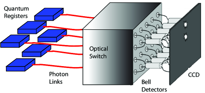
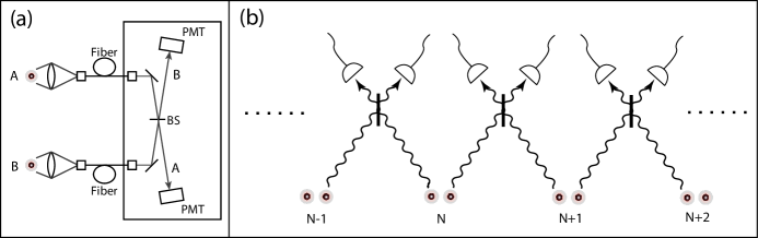
A higher level architecture for entangling an arbitrary number of atomic qubits is an atom–photon network [10, 11, 12, 13, 14], in which singular or locally interacting material qubits form the quantum registers of a distributed quantum network as depicted in Fig. 1. The modular structure of this network relies on entangling atomic qubits with photonic qubits in order to establish entanglement between the quantum registers. Here, we concentrate on probabilistic links where the atom–photon entanglement process succeeds with a low probability, yet this probabilistic process still can be used to to generate arbitrary-size quantum networks [15].
Central to the idea of a probabilistic atom–photon network is the heralded entanglement process between remote nodes, which includes the following two steps. First, the scattering of photons establishes entanglement between atomic and photonic qubits. Second, the interference and detection of the scattered photons from multiple atomic qubits project the remote atomic qubits into an entangled state. The success probability for the first step is
| (1) |
where is the probability of generating the desired entangled atom–photon pair, is the efficiency of collecting the emitted photon by the optical system, and is the transmission efficiency of the entire optical system, including fiber coupling. The second step of the heralded entanglement adds other factors to the success probability, including the loss of certain photonic states at the Bell state detector [16] and the quantum efficiency of the photon detectors. Experiments demonstrating entanglement between two remote ions [17, 18, 19, 20] have clearly shown that the light collection efficiency is the leading limiting factor for the overall success probability. Improvements to the light collection efficiency from trapped ions therefore play a crucial role for creating a scalable and efficient atom–photon quantum network.
In this paper, we review protocols and techniques suitable for constructing a scalable atom–photon quantum network. We first provide a detailed description of methods to create entangled atom–photon pairs with different types of photonic qubits (Sec. 2), as well as protocols for generating heralded entanglement and operating quantum gates between two remote atomic qubits (Sec. 3). Where applicable, we will provide examples with ions as quantum memories. To apply these schemes for building large–scale atom–photon networks, we discuss specific protocols and techniques relevant to trapped ions, including using photon emission from multiple ions to entangle a linear crystal of ions (Sec. 4) and improving light collection from trapped ions by reflective optics or an optical cavity (Sec. 5). We also present a brief outlook of a scalable atom–photon network for quantum information processing (Sec. 6).
2. Protocols for Generating Atom–Photon Entanglement
Entangled atom–photon pairs can be generated from a wide range of systems, including trapped ions, neutral atoms, and atomic ensembles [12]. The quantum protocols used to produce these entangled pairs are general and not limited to the specific systems. In this section, we first review these general protocols, and then use trapped ions as an example to show detailed schemes of generating both ultraviolet and infrared photonic qubits.
2.1. Types of Photonic Qubits
When a laser pulse hits an atom, photons can be scattered through either a resonant or off-resonant process. In both processes the atom can be transferred from the initial state to the multiple final states through different scattering channels. If an atom has two distinct scattering channels correlated with two orthogonal states of the scattered photon, an entangled atom–photon pair is produced as described by
| (2) |
where and represent the atomic qubit state, and and are the orthogonal states of the photonic qubit. The values of the probability amplitudes, and , depend on the specific scheme used to generate the entangled pairs.
The physical properties of photons that are most often used to encode the photonic qubits are (i) existence of the photon(s) (number qubits), (ii) polarization, (iii) frequency, and (iv) the emission time (time-bin qubits).
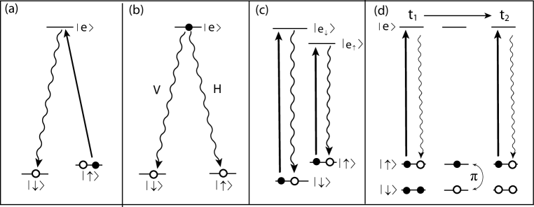
Number Qubits. Suppose a three-level atom with a ‘ configuration’ is initially prepared in one of its ground states, , as shown in Fig. 2(a). Photons in a laser pulse are scattered by the atom, transferring the atom from to with certain probability . After the scattering, the final atom–photon state is described by
| (3) |
conforming to Eq. 2. Here and denote the vacuum state and the one photon state generated by the scattering process.
Polarization Qubits. Polarization qubits can be realized by the scheme shown in Fig. 2(b). An atom, initially prepared in the excited state , spontaneously decays to the ground states and with probability and , respectively. Each decay channel is associated with a polarization component of the emitted photon. If these two polarization components, denoted by and , are orthogonal, the atomic qubit stored in the and states is entangled with the polarization of the emitted photon. The overall atom-photon state is described by
| (4) |
conforming to Eq. 2. Here and denote the and polarization states for a single photon.
Frequency Qubits. One example of generating frequency qubits is shown in Fig. 2(c), where both the ground state and the excited state have two non-degenerate energy levels. Frequency qubits can also be generated by addressing only one energy level in the excited state, but this configuration does not support a quantum gate operation [17]. In the case shown in Fig. 2(c), the four energy levels are chosen so that selection rules only permit transitions from and . The atom is initially prepared in an arbitrary superposition state, . A laser pulse, whose bandwidth covers both the transitions, coherently excites the atom to the state. The population in each excited state then decays back to its initial ground state. Because the frequency of the spontaneously emitted photon is uniquely correlated with the originally prepared quantum state, this process results an entangled atom–photon pair given by
| (5) |
conforming to Eq. 2. Here and denote the one-photon states for two different frequency components, where is the red, or low frequency photon, and is the blue, or high frequency photon. These frequency qubit states are resolved when , where and are the two photon frequencies and is the linewidth of the transitions. We note that the final entangled state preserves the quantum information in the initial qubit state, thus admitting quantum gate operations.
Time-bin Qubits. The time at which a photon is emitted can also be used to encode photonic qubits [21, 22]. This type of photonic qubit is defined by a superposition of states in which a photon exists within a ‘time bin’ centered either at time or . The time-bin states are resolved when . As shown in Fig. 2(d), an atom is initially prepared in a superposition state of . The excited energy level is chosen so that the selection rules only permit the transition from . At time , a single frequency laser pulse resonant with the transition excites the population to the state. After the population in the excited state decays, the atom–photon state is , where and represent the one-photon state and the vacuum state at time . A pulse is then applied to rotate the atomic qubit, changing the atom–photon state to . At time , a second resonant laser pulse is applied to again excite the population in the state. Following the spontaneous decay, the final entangled atom–photon state is given by
| (6) |
conforming to Eq. 2. Here and represent the states of a single photon at time and .
2.2. Photonic Qubits for Ions
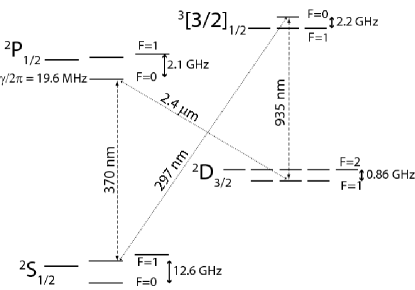
All the atom–photon entanglement schemes discussed above can be realized through resonant scattering processes with laser-cooled, trapped ions [23]. Table 1 details how the four types of photonic qubits illustrated in Fig. 2 can be created using the transition of ions in the ultraviolet (UV) at nm. Polarization and frequency photonic qubits have been realized experimentally in Ref. [17, 18, 19, 20].
| Photonic Qubit Type | Ground State | Excited State |
|---|---|---|
| Number Qubit | ||
| Polarization Qubits | ||
| Frequency Qubits | ||
| Time-bin Qubits | ||
We note that the system also supports infrared (IR) photonic qubits, which may be useful for long-distance quantum communication. Moreover, access to additional optical frequencies may facilitate entanglement between disparate optically active systems (e.g. between trapped ions and quantum dots). IR photonic qubits can be generated by either the transition (935 nm) or the transition (1.3 µm), as shown in Fig. 4 for polarization and frequency photonic qubits.
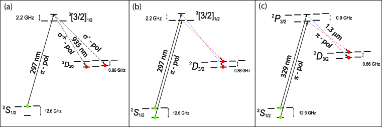
The branching ratio of the level between and has been calculated to be about 55:1 [24], which decreases the probability of generating a 935 nm photon and thereby reduces the overall success probability of the entanglement protocols discussed below. Two potential experimental problems arise from the small branching ratio. First, a higher fraction of the detection events will be dark counts due to the additional detector integration time. However, there is a way to “veto” these extra dark counts. After a 935 nm photon detection event, a pulse at the hyperfine splitting can be used to coherently shelve the qubit state populations to the manifold. If the fluorescence detection procedure detailed in [23] is now performed, in which population of is undisturbed, no 370 nm photons should be detected. The detection of 370 nm photons during this interval would indicate that the 935 nm photon “detection” was in fact a dark count and should be discarded. The atomic population transferred from to can then be returned by a second microwave pulse. The second problem posed by the small branching ratio is that it is difficult to implement state detection for atomic qubits by using the 935 nm infrared transition directly. Instead, the states can be mapped to the states so that the aforementioned UV photon fluorescence detection can be used to measure the atomic qubits. For example, to detect the atomic states described in Fig. 4(a), the population in the state could be transferred to the manifold by a resonant microwave pulse at the hyperfine splitting of 0.86 GHz. Light from a 935 nm laser could transfer the population from the manifold to (Fig. 3). The state of the atom is then determined by resonantly driving the transition and detecting the fluorescence, indicating the atom was originally in the state.
Finally, we consider the 1.3 µm photons generated from the to transition. The branching ratio from to versus is about 475:1 [24]. While the 1.3 µm wavelength is more amenable to long distance transmission, the decrease in the protocol success probability is even more drastic. In addition, can also decay to , which can subsequently decay to the long-lived state. Depopulating these additional metastable states could limit the repetition rate of the experiment.
3. Protocols for Generating Remote Atom–Atom Entanglement
The entangled atom–photon pairs described in the last section can be used to entangle two remote non-interacting atomic qubits. The key component of entangling these atomic qubits is the interference of the photons on a 50:50 beamsplitter as shown in Fig. 5(a). In contrast to post-selected entanglement schemes, in which measurement of the entangled qubits destroys the entanglement, the detection of photons after the beamsplitter destroys only the photonic system, which can herald the projection of the atomic states into an entangled state. This heralded entanglement technique generates useful entangled atomic pairs that serve as the chief resource for constructing a photon-mediated quantum network.
There are two types of heralded entanglement, distinguished by whether only one photon is emitted by the two atoms (type I) or one photon is emitted by each of the two atoms (type II) [10]. For a single photon input state [25, 11], the output of a 50:50 beamsplitter is given by
| (7) |
As shown in Fig. 5(a), denotes the number of photons and in the two spatial modes and entering or emerging from the beamsplitter, having the same frequency and polarization. For a two-photon input state [25, 11], the interference generates the output states
| (8) |
3.1. Type I Heralded Entanglement
To implement the type I heralded entanglement protocol, laser pulses are applied to two atoms and so that , as shown in Fig. 2(a). The scattering process yields two entangled atom–photon pairs with states . The state of the two atom–photon pairs and is then
| (9) | |||||
where terms of order and higher are ignored. The relative phase , where is the wavevector difference between the excitation laser and the collected photons, and is the optical path lengths difference from the atoms to the beamsplitter. After the beamsplitter, the output state containing one photon is
| (10) |
This result indicates that once the two PMTs detect one photon, the atom–atom state is projected into one of the following states
| (11) |
where the sign is determined by which PMT detects the photon.
The success probability of type I entanglement is , where is the success probability of obtaining a useful atom–photon entangled pair (Eq. 1) and is the photon detection efficiency. According to the above analysis, there is a small probability of order that both atoms scatter photons. If only one photon is detected, there is still a probability that another photon was emitted but not detected, representing a limit on the fidelity of this entanglement procedure.
Type I entanglement relies on interferometric stability of the optical paths, so fluctuations in the phase must be kept small. An important source of decoherence is the atomic recoil from the absorption and emission of a photon, indicating which atom scatterers the photon [26, 27]. The resulting entanglement fidelity is found to be in the Lamb-Dicke limit where [28]. Here, is the Lamb-Dicke parameter of each ion of mass , and is the average number of thermal quanta of motion in a trap of frequency . This problem can be overcome by collecting photons in the forward scattering direction (), or by confining the ions deeply within the Lamb-Dicke limit where the recoil probability is small.
3.2. Type II Heralded Entanglement and Gate Operation
The interferometric stability requirement for type I entanglement is a serious challenge for experimental implementation. Type II entanglement bypasses this issue through interference of two photons, one from each atom, where the interferometric phase becomes common mode. This makes type II entanglement more robust to noise, and it has been successfully demonstrated in experiments [17, 18, 19, 20].
Polarization, frequency, and time–bin qubits can all be used for type II entanglement generation. Frequency and time–bin qubits can also be used to implement a heralded quantum gate, where the output state depends on the input state of the atomic qubits. We discuss this gate operation, and show how it can be used for entanglement generation.
Initially atoms and are independently prepared in arbitrary quantum states. The total atom–atom state is described by
| (12) |
Suppose the entangled atom–photon pairs are generated, preserving the initial quantum information by using appropriate photonic qubits. If we assume equal optical path lengths from each atom to the beamsplitter for simplicity, the overall input state of the atom–photon pairs to the beamsplitter is
| (13) | |||||
| (14) |
where and are the maximally entangled Bell states for photonic qubits and and are the associated atomic states given by
| (15) | |||||
| (16) | |||||
| (17) | |||||
| (18) |
As a consequence of the quantum interference at the beamsplitter, the photons will emerge from different exit ports only if they are in the antisymmetric state [29, 30, 16, 25]. Using frequency qubits as an example, where and , according to Eq. 7, the beamsplitter produces the output state
| (19) |
Consequently, when the two PMTs detect a coincident event, the final atom–atom state is projected into
| (20) |
The above protocol generates the final state from the initial state by a gate operation given by
| (21) |
where is the single qubit Pauli-z gate for atom (). Notice that this gate is not a unitary operator since the input states and do not output any heralded events, yielding a null result. This quantum gate operation can be used to entangle two atomic qubits: for example, if the initial state is set to in Eq. 12, the gate operation generates a maximally entangled Bell state.
There are some advantages to performing type II entanglement with time–bin qubits. First, in contrast to frequency and polarization qubits, photons in time–bin qubits have only one component mode of polarization and frequency and are less sensitive to birefringence and dispersion in the photonic channel. This feature also makes time–bin qubits a good candidate for generating entangled atom–photon pairs using a cavity setup as discussed in Sec. 5.2. Second, the system can be projected into either the or the state by using time–bin qubits, where and . Note that this is a consequence of PMTs being able to resolve the arrival time of photons but not the frequency. From Eq. 7, the output states from the beamsplitter for are given by
| (22) | |||||
| (23) |
This explicitly shows that if only one scattered photon is detected at each time and by different PMTs, the photon state is projected into the state, which projects the atom–atom state into the entangled state . Instead, if the events are detected by the same PMT, the photon state is projected into the state, yielding the atom–atom state .
Since type II entanglement schemes require the presence of two photons, the success probability is , where is the probability of detecting a Bell state of the two photons (in the examples above, for the frequency qubit and for the time-bin qubit). The success probability for type II entanglement is quadratic in and is thus typically much smaller than that of type I for . However, type II entanglement has the advantages of no fundamental fidelity limit and far less sensitivity to experimental noise and interferometric instability.
If the path length difference between the two photonic channels is offset by an amount , a phase factor emerges between the two components of Eq. 20. For frequency photonic qubits, is the difference frequency between the two photon frequencies, and for time-bin qubits this is given by the frequency difference between the atomic qubit levels. Since , type II entanglement and gate operation are typically much more robust than type I schemes.
4. Quantum Information Protocols Based on Multi-ion Emission
Photon emission from multiple ions can be a useful technique to scale up the type I entanglement protocol to create large multi-partite entangled states. In this section we focus on the type I scheme to entangle many atoms through the collective emission of one photon. This entanglement protocol can be used to generate multi-partite entangled W-states [28, 31]. W-states have been shown to provide a means to secure quantum communication [32], and have also been proven to be the only state capable of solving certain problems on quantum networks [33]. Besides these specific applications, the W-state may be of interest for investigating emergent phenomena in large multi-partite entangled states[34].
-particle W-states of the form can be created by weakly exciting atoms such that the probability to scatter more than one photon is vanishingly small [28]. The notation refers to generalized W-states, in which the phase factors present in the quantum state are arbitrary but fixed. The specific state where all the phase factors are equal is simply referred to as the W-state . Implementing such a type I process with remotely-located ions will come at the cost of maintaining optical interferometric stability, so we consider the heralding of W-states by using atoms confined in a single trap. The generation of a N-atom W-state can be verified by measuring the entanglement witness given by , the negative expectation value of which signals multi-partite entanglement [35]. By exploiting the symmetry of the W-state with respect to an exchange of any two qubits, it was shown that this witness operator can be measured by measurements without individual addressing [36]. Because the phase factors of the W state are determined by the relative optical path lengths from each ion to the detector, the angular distribution of the scattered photon forms interference fringes. In order to use this witness to characterize the entanglement, the photon detector must be able to resolve these fringes.
We develop a method of calculating the fidelity of the W-state by drawing a parallel between the storage of coherence in the atoms through an inelastic scattering event and the coherence in the light field through an elastic scattering event. In the experiment of Ref. [26], where two ions in a single trap were weakly excited, the position of scattered photons was shown to exhibit interference in elastic scattering events but no interference in inelastic scattering events. In the case of elastic scattering, no information about which ion scattered the photon will exist, allowing the different optical paths to interfere [26, 37]. This process yields an interference pattern with regions of high intensity, where the photon phases add constructively. In the case of inelastic scattering, the photon phase gets imprinted on the ions upon detection of a photon. The ions will also pick up a dynamical phase , where is the time it takes for the photon to reach the detector, and is the frequency difference between and . If the time that photons take to traverse the full length of the ion crystal is short compared to , this dynamical factor can be ignored. For the Zeeman splitting with a magnetic field on the order of a few Gauss, this approximation is valid for ion crystals much smaller than one meter. When this approximation is valid, the regions of high intensity in the elastic case are the same points at which the detection of a photon in the inelastic case signals the creation of a W-state with all the phases being equal. Therefore, in order to identify scattering regions that herald a high fidelity W-state, it should suffice to calculate the elastic scattering cross-section for ions in a trap and identify the high intensity region.
In order to find the points of high intensity in the radiation pattern, we generalize the derivation of the scattering cross-section for two ions in a single trap [27] to ions. Starting with the differential scattering cross-section as given by the electric dipole Hamiltonian in second-order perturbation theory
| (24) |
where and are the dipole and position operators for the ion, is a polarization vector, and are incoming and outgoing wavevectors and the indices and represent the initial and final state of the ions. It is important to note that this expression only applies to elastic scattering events, since in this case the probability amplitudes for the photon scattering off different ions are added together because these processes are indistinguishable. The quantum states in the perturbation expansion are taken to be eigenvectors of the unperturbed Hamiltonian of ions in a harmonic trapping potential and are therefore product states of the ions’ internal degrees of freedom and the motional state of the system.
We now examine the special case of the ion crystal axis lying in the plane defined by the incoming and outgoing wavevectors and the quantization axis being perpendicular to that plane. In this case, the dipole operator only contributes an overall scaling factor to the scattering cross-section and is therefore ignored in this calculation. As explained in [27], the denominators in Eq. 24 are nearly constant for the ion cooled near the Doppler limit on the nm line as a consequence of the recoil frequency, kHz, being small compared to the linewidth. By considering the denominators to be nearly constant, they can be factored out of the sum allowing us to do the sums over the and indices via resolutions of the identity operator, giving
| (25) |
where denotes the initial harmonic oscillator quantum numbers of the ions. Eq. 25 might be seen as a classical interference pattern from a diffraction grating comprised of slits that oscillate around fixed points and recoil upon deflection of light quanta. After taking the expectation value, the final scattering cross-section is given by
| (26) |
In the above equation, are the average number of axial (transverse) thermal quanta in mode and . is a vector containing the equilibrium positions of the ions in units of length . The Lamb-Dicke parameter for the mode in the axial (transverse) direction is denoted . The difference between incoming and outgoing wavevectors is , and are elements of transformation matrices from position coordinates to axial and transverse normal coordinates, respectively.
The fidelity of the entangled state with arbitrary phase of two ions in separate isotropic harmonic traps (frequency and average thermal index ) as derived in Ref. [28] is given by
| (27) |
with and being the angle between the excitation beam and the emission direction. In the limit of weak confinement, , and because the integrand decays exponentially in , we can approximate , allowing us to carry out the integration and arrive at
| (28) |
This shows the relationship between Eq. 27 and the contrast of the fringes in Eq. 26. This suggests that the fringe contrast of Eq. 26 for might be interpreted as the fidelity of the entangled state with arbitrary phase when two ions are in the same trap. Moreover, because the fringe peaks correspond to points of common phase, the full expression (Eq. 26) for might be interpreted as the fidelity of the state where the relative phase is equal to zero. We contend that Eq. 26 should be a valid prediction of the fidelity of an qubit W-state in the weak confinement regime, with ensuring no ion–ion photon exchange.
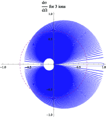
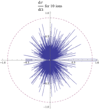
In Fig. 6(a) the emission pattern for three ions is plotted, clearly showing the degrading effect of recoil due to a large scattering angle. As a consequence of the ions not being evenly spaced, the scattering profile from ten ions in Fig. 6(b) shows that the only points where radiation adds up in phase is in the forward scattering direction. This implies that in an inelastic scattering event, the only points where light detection will yield a W-state with all the terms having the same phase is in the forward scattering direction. The angular size of this spot, , in the case where the excitation pulse is along the crystal axis can be estimated by first normalizing Eq. 26 by dividing by , ignoring the Debye-Waller factors and making the small scattering angle approximation, giving
| (29) |
The sum in Eq. 29 can be approximated by numerically solving for the equilibrium positions for different numbers of ions in a harmonic trap, which yields . We define the spot size to be the region where the intensity is at least times the maximum and find the angular size of the spot to be approximately given by
| (30) |
Remembering that the entanglement witness demands that the fidelity of the W-state be bounded by , we set . With the interpretation that the elastic scattering cross-section represents the fidelity of the W-state for an inelastic scattering event, the fraction of photons scattered into the plane of interest that will yield an particle W-state is solved
| (31) |
Eq. 31 allows the estimation of an upper bound on the angle subtended by the detector being used to signal the creation of a multi-partite entangled state. This scaling law shows that the efficiency with which one can create multi-partite entanglement decreases rather slowly with the number of entangled ions.
5. Techniques for Enhancing Light Collection
Collecting spontaneously emitted photons from trapped atomic ions traditionally involves the use of refractive optics in free space. A common setup uses a high numerical aperture objective to collect light for entanglement protocols as well as state detection. For the entanglement protocols discussed in Sec. 2, mode matching of the photons is critical, so light is typically coupled into single-mode optical fibers. For this type of free-space light collection, there are two critical difficulties that limit the collection efficiency. First, the solid angle subtended by the collecting lens, , is usually on the order of [19]. This small collection angle contributes a factor of order to the total success probability for type II heralded entanglement schemes. Second, the mode overlap of the optical dipole mode to the fiber mode substantially decreases the amount of light transmitted by the optical system.
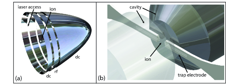
In recent years many proposals for enhancing atom–photon coupling have emerged [38, 39, 40, 41, 42, 43]. In Fig. 7 we show two possibilities of employing either reflective optics or an optical cavity to increase light collection efficiency. One option is to use a single parabolic mirror to collect a large fraction of the scattered light from the atom [39]. Another method is to place the atom inside a high finesse optical cavity and utilize the Purcell effect to extract photons. For this application, the strong coupling regime is not necessary. Instead, the perturbative regime, or “bad cavity” limit (Sec. 5.2), will suffice, as long as the coherent coupling rate is larger than the dipole decay rate.
Ion traps suitable for such experiments would necessarily need to have an optically open geometry, such as a surface trap [44, 45] or a needle trap [46, 47], to minimize the occlusion of light reflected from a mirror or the optical mode of the cavity. The radio frequency (RF) node of the ion trap must be precisely placed at the focus of the reflective mirror or along the cavity axis. The ion trap could be monolithically created, ensuring precise alignment of the RF node with the optical field, or it could be aligned in situ. For dielectric optics, the characteristic ion–electrode distance must be much smaller than the ion–optic spacing in order to provide adequate shielding of the ion from potential charge accumulation on the optic. Fig. 7 is a conceptual view of an ion confined at the the focus of a parabolic reflector trap (Fig. 7a) or in an optical cavity (Fig. 7b).
5.1. Reflective Optics
One way of collecting more light emitted by a single trapped ion is to place the minimum of the trapping potential at the focus of a parabolic mirror. In this section we analyze the fiber-coupling efficiency of the dipole radiation from an ion at the focus of such a trap, with its quantization axis along the line of symmetry.
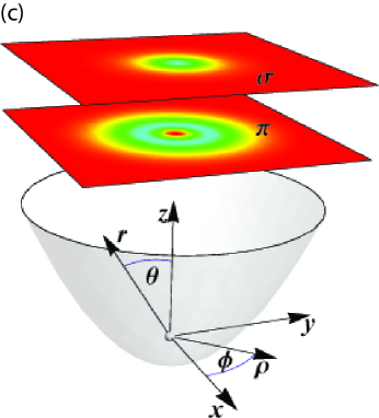
Prior to reflection, the optical fields of emitted photons associated with the three possible transitions are given by
| (32) |
Once the light has reflected and formed a collimated beam, the wavefronts are flat, meaning the exponential factor will be a constant and can be ignored.
Using polar coordinates shown in Fig. 8, the paraboloid is defined by , and the distance from the ion to the reflecting surface is then given by . After reflection, light that was polarized in the direction will have polarization in the direction, while the polarization is unchanged. The intensity profile that was only a function of will be mapped to an intensity profile that only depends on . The mapping can be found by solving for the distance from the symmetry axis after reflection as a function of the angle of emission, giving .
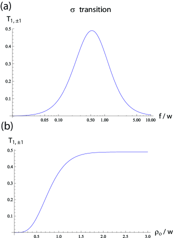
As shown in Eq. 33, the transition will produce a donut mode with radial polarization given by
| (33) |
which is consistent with the optimal intensity profile for driving a transition derived in [39]. The amount of light from this mode that will couple into a single mode fiber is given by the mode overlap
| (34) |
where the quantity is the maximum radius of the mirror being used and is the Gaussian mode of the fiber where . Assuming the intensity and polarization of the Gaussian mode only depend on , the only dependence of the integrand in the numerator on the angle is in the unit vector , causing the integral to vanish. Therefore, without additional optics, there will be no transmission of transition light into a fiber aligned with the axis of symmetry.
After reflection, the field for a transition is given by
| (35) |
The collimated beam has circular polarization in the center, becomes increasingly elliptical going away from the center until it is azimuthally polarized at a distance of , then becomes elliptical again approaching a polarization orthogonal to the center of the beam. The overlap integral is calculated using Eq. 35 to give the following coupling efficiency
| (36) |
where is the incomplete Gamma function. This expression shows that the light from the transition coupling to the fiber has left-handed polarization, and the light generated from the transition coupling to the fiber has right-handed polarization. If we take the limit where the paraboloid has infinite extent, we can numerically solve for the focus that gives maximum coupling efficiency. Fig. 8 shows the results of this calculation, which predicts a maximum coupling efficiency near .
This setup may also be used for the logic gate described earlier using frequency qubits. Because the transition light does not couple into the fiber without additional optics, we consider transitions. In order to preserve any initial coherence set up in the ion after excitation and emission, we can use the transitions in the ion. The fields resulting from these transitions are superpositions of Eq. 35. Because the fiber maps the transition photons to circularly polarized photons while preserving orthogonality, a photon captured by the fiber will have a linear polarization orthogonal to a photon captured by the fiber. With this setup, we can still use the clock states in the ground state manifold to hold quantum information, but now we use light to couple to the Zeeman states in the manifold. Here, the two states are coupled to the excited state with polarization, respectively. This implies that after excitation and decay the internal state of the ion will be correlated with both the frequency and polarization of the emitted photon. In order to use the parabolic mirror for the gate, the polarization information should be erased to allow for the interference on the beam splitter to occur. The distinguishability between the and transitions can be erased with a linear polarizer oriented to block . Assuming perfect coupling into the fiber, the probability to see a coincidence is now given by , where the three factors of come from maximum coupling efficiency, Clebsch-Gordan coefficients, and the polarization erasure.
5.2. Optical Cavity
Another method to increase light collection is to surround the ion with an optical cavity [48, 49, 50]. The field mode modifications imposed by the mirrors change the spontaneous emission of the ion such that it preferentially emits into the cavity mode, depending on the coupling parameters. This phenomenon is the well-known Purcell effect [51].
The dominant ion–cavity coupling parameters are the coherent atom–field coupling, , the free space ion spontaneous emission rate, , and the cavity decay rate, . These parameters define the cooperativity, , which is a measure of the atom-cavity coupling with respect to the dissipative processes. The atomic spontaneous emission rate is enhanced by a factor proportional to . If we assume that the photon collection efficiency equals the probability of a spontaneously emitted photon emerging from the outcoupling mirror of the cavity, over experimental time scales, the collection efficiency is given by
| (37) |
The first factor, is the fraction of light that is transmitted by the outcoupling mirror, , to the total losses of the cavity . The second factor relates the rate photons leave the cavity to the rate they leave the ion–cavity system. The third factor is the fraction of light scattered into the cavity mode. The “bad cavity” regime can be intuitively envisioned as providing enough atom–cavity coupling to transfer the excitation from the atom into an entangled atom–photon pair. This photon then leaves the cavity faster than the time it takes to be reabsorbed by the atom and emitted into unwanted side modes.
An optical cavity can be used for all the protocols discussed in Sec. 2. Number qubits can be realized with the coherent transfer of an excitation from the atom to a single mode of the cavity [52, 38, 50]. Polarization qubits can be realized with a cavity coupling to Zeeman levels of atoms lying inside the linewidth of the cavity [53]. Frequency qubits would need both frequency modes resonant with the cavity. A difficulty with realizing frequency qubits is the dependence of the coherent coupling strength, on the mode volume. In order to ensure that is an integral multiple of the free spectral range it may be necessary that the cavity length be large. However, a longer cavity tends to have a larger mode volume, leading to a smaller coupling strength . A method to combat this is a near-concentric geometry. In this case, the centers of curvature of the two mirrors nearly coincide. This leads to an optical mode with an extremely tight focus, allowing a relatively strong coupling strength . Time-bin qubits can use the frequency selectivity of the cavity to ensure that one of the transitions is off-resonant [22]. However, to preserve the coherence, one must be careful not to excite both levels. That is, the excitation pulse must have a bandwidth much smaller than the qubit spacing, yet the bandwidth must be greater than the excited state linewidth.
6. Outlook and Conclusions
The quantum network generated by photon-mediated entanglement can be used for quantum communication and distributed quantum computation. We list some possible applications for such an atom–photon network.
Loophole-free Bell Inequality Test. Loophole-free Bell inequality tests are of continuing interest for testing fundamental aspects of quantum mechanics[54]. Bell inequality violation experiments are subject to two primary loopholes: the detection loophole, and the locality loophole [55, 56]. While trapped ions typically close the detection loophole due to nearly perfect state detection, they have yet to close the locality loophole. On the other hand, photonic qubits enable the separation required to close the locality loophole, yet cannot be detected efficiently enough to close the detection loophole. Combining the advantages of both trapped ion and photons, the photon-mediated entanglement schemes discussed above can generate an entangled ion pair that could close both loopholes [57]. To close the locality loophole, the remote ions must to be space-like separated; that is, the ions must be separated greater than the distance light travels in the time it takes to perform state detection. For example, if the state detection time were s, then the ions would need to be separated by . Since the starting point for a Bell inequality measurement is the heralding of the remote entanglement, the success probability does not play a role in determining the separation of the two ions. However, the improvements to the photon collection efficiency, , can shorten the state detection time, thus reducing the space separation between two ions.
Remote Deterministic Quantum Gates and Quantum Repeaters. The photon-mediated entanglement schemes can also be used to build a quantum repeater to transmit quantum information across long distances [58, 59], as well as to create a deterministic controlled-not gate between two non-interacting ions [10]. An array of ion traps each containing a logic ion and an ancilla ion, as illustrated in Fig. 5(b), can be used to perform a remote deterministic gate. Here, the logic ions contain quantum information, while the ancilla ions are used to create a photon-mediated channel whereby a gate can be performed. These remote deterministic gates are created by four consecutive steps: (1) a probabilistic scheme is applied to two ancilla ions until their entanglement is heralded; (2) local deterministic controlled-not gates are performed on each logic and ancilla qubit pairs; (3) the ancilla qubits are measured in an appropriate basis; (4) single qubit rotations on the logic qubits are applied based on the results from the measurements of ancilla ions. The expected number of attempts for a successful entanglement of the ancilla ions is , depending on the success probability of the two-qubit entanglement scheme. Hence, the average time required to perform a deterministic remote gate is .
This scheme can be extended to create a quantum repeater. Again, we consider a chain of ion traps spanning the distance, , over which the information needs to be sent. In each trap there are two ions, one to generate a link between each of the adjacent nodes. For example, in the node, photon-mediated entanglement links one ion to the node, and the other ion links the node. A joint Bell state measurement on the node leaves the node entangled with the node, thereby increasing the distance between entangled nodes. The time required to generate entanglement over a distance with nodes is thus .
Generation of Cluster States. These photon-meditated quantum networks provide a compelling possibility for operating a large–scale quantum computer. One universal quantum computation model is the measurement based cluster state model, which uses a highly entangled state as an input resource [60, 61]. This model requires an initial generation of a large–scale two-dimensional cluster state and individual single qubit rotations and measurements.
The heralded gate operation discussed earlier (Eq. 21) is not unitary gate, which prevents its application to the quantum circuit model. However, this gate can be used to generate cluster states because the input qubits for constructing the cluster state are required to be a superposition state, and the gate will never give a null result in this case [62].
A 2D square lattice cluster state can be prepared with probabilistic gates that succeed with probability [15]. Considering a (small) overall failure probability for an -qubit square lattice cluster state, the required time to generate the state is
| (38) |
where is the operation time for a single attempted gate operation. From the above equation, the time required to generate a cluster state is almost independent on the number of cluster nodes . For example, with and a two-qubit gate success probability and s for the heralded gate discussed above, we find that the time required for generating the cluster stare with and only differs by . However, the temporal resource strongly depends on the success probability . With , this protocols needs about 5900 years to generate a 2D square lattice cluster state with nodes, compared with a time of 0.16 second with . This shows how critical the improvement of the heralded gate success probability is for constructing a large scale quantum network.
In this paper, we have described various protocols that rely on spontaneous emission processes and single photon interference effects to generate atom–photon and atom–atom entanglement. Variant schemes, such as generating infrared photonic qubits and collecting multi-ion emission, have also been studied. We emphasize that currently the primary issue for realizing a scalable atom–photon quantum network is the improvement of the probability of collecting spontaneous emitted photons from trapped ions. To realize this goal, reflective optics and optical cavities are suggested for integration into trapped ion systems to enhance the light collection efficiency. We expect that even a modest improvement to this efficiency can lead to a large improvement in the success probability of entangling two distant atomic qubits. Such improvements also increase the feasibility of deterministic quantum gate operations between remote atomic qubits, quantum repeater networks, and cluster state generation.
This work is supported by IARPA under ARO contract, the NSF Physics at the Information Frontier Program, and the NSF Physics Frontier Center at JQI. L.L. is supported by JQI postdoctoral fellowship.
References
- [1] D. P. DiVincenzo, Fortschritte der Physik 48, 771 (2000).
- [2] C. Monroe and M. Lukin, Physics World August, 32 (2008).
- [3] R. Blatt and D. Wineland, Nature 453, 1008 (2008).
- [4] H. Häffner, C. Roosa, and R. Blatt, Physics Report 469, 155 (2008).
- [5] D. Leibfried, B. DeMarco, V. Meyer, D. Lucas, M. Barrett, J. Britton, W. M. Itano, B. Jelenkovi, C. Langer, T. Rosenband, and D. J. Wineland, Nature 422, 412 (2003).
- [6] F. Schmidt-Kaler, H. Häffner, M. Riebe, S. Gulde, G. P. T. Lancaster, T. Deuschle, C. Becher, C. F. Roos, J. Eschner, and R. Blatt, Nature 422, 408 (2003).
- [7] P. C. Haljan, P. J. Lee, K. A. Brickman, M. Acton, L. Deslauriers, and C. Monroe, Phys. Rev. A 72, 062316 (2005).
- [8] J. P. Home, M. J. McDonnell, D. M. Lucas, G. Imreh, B. C. Keitch, D. J. Szwer, N. R. Thomas, S. C. Webster, D. N. Stacey, and A. M. Steane, New J. Phys. 8, 188 (2006).
- [9] D. Kielpinski, C. Monroe, and D. Wineland, Nature 417, 709 (2002).
- [10] L. M. Duan, B. B. Blinov, D. L. Moehring, and C. Monroe, Quant. Inf. Comp. 4, 165 (2004).
- [11] D. L. Moehring, M. J. Madsen, K. C. Younge, R. N. Kohn, P. Maunz, L. M. Duan, C. Monroe, and B. Blinov, J. Opt. Soc. Am. B 24, 300 (2007).
- [12] L. M. Duan and C. Monroe, Advances in Atomic, Molecular, and Optical Physics 55, 419 (2008).
- [13] H. J. Kimble, Nature 453, 1023 (2008).
- [14] J. Kim and C. Kim, Quant. Inf. Comp. 9, 181 (2009).
- [15] L. M. Duan and R. Raussendorf, Phys. Rev. Lett. 95, 080503 (2005).
- [16] S. L. Braunstein and A. Mann, Phys. Rev. A 51, R1727 (1995).
- [17] D. L. Moehring, P. Maunz, S. Olmschenk, K. C. Younge, D. N. Matsukevich, L. M. Duan, and C. Monroe, Nature 449, 68 (2007).
- [18] D. N. Matsukevich, P. Maunz, D. L. Moehring, S. Olmschenk, and C. Monroe, Phys. Rev. Lett. 100, 150404 (2008).
- [19] S. Olmschenk, D. N. Matsukevich, P. Maunz, D. Hayes, L. M. Duan, and C. Monroe, Science 323, 486 (2009).
- [20] P. Maunz, S. Olmschenk, D. Hayes, D. N. Matsukevich, L. M. Duan, and C. Monroe, arXiv:0902.2136 (2009).
- [21] J. Brendel, N. Gisin, W. Tittel, and H. Zbinden, Phys. Rev. Lett. 82, 2594 (1999).
- [22] S. D. Barrett and P. Kok, Phys. Rev. A 71, 060310(R) (2005).
- [23] S. Olmschenk, K. C. Younge, D. L. Moehring, D. N. Matsukevich, P. Maunz, and C. Monroe, Phys. Rev. A 76, 052314 (2007).
- [24] E. Biémont, J. F. Dutrieu, I. Martin, and P. Quinet, J. Phys. B: At. Mol. Opt. Phys. 31, 3321 (1998).
- [25] L. Mandel, Rev. Mod. Phys. 71, S274 (1999).
- [26] U. Eichmann, J. C. Berquist, J. J. Bollinger, J. M. Gillingan, W. M. Itano, D. J. Wineland, and M. G. Raizen, Phys. Rev. Lett. 70, 2359–2362 (1993).
- [27] W. M. Itano, J. C. Berquist, J. J. Bollinger, and D. J. Wineland, Phys. Rev. A 57, 4176 (1998).
- [28] C. Cabrillo, J. I. Cirac, P. Garcia-Fernandez, and P. Zoller, Phys. Rev. A 59, 1025 (1999).
- [29] C. K. Hong, Z. Y. Ou, and L. Mandel, Phys. Rev. Lett. 59, 2044 (1987).
- [30] Y.H.Shih and C.O.Alley, Phys. Rev. Lett. 61, 2921 (1988).
- [31] D. Kielpinski, New J. Phys. 9, 408 (2007).
- [32] J. Jaewoo, J. Lee, J. Jang, and Y. Park, arXiv:quant-ph/0204003.
- [33] E. D’Hondt and P. Panangaden, Journal of Quantum Information and Computation 6(2), 173 (2005).
- [34] P. C. W. Davies, Fluctuation and Noise Letters 7(4), C37 (2007).
- [35] M. Bourennaneand, M. Eibl, C. Kurtsiefer, S. Gaertner, H. Weinfurter, O. Gühne, P. Hyllus, D. Bruß, M. Lewenstein, and A. Sanpera, Phys. Rev. Lett. 92, 087902 (2004).
- [36] O. Gühne, C. Lu, W. Gao, and J. Pan, Phys. Rev. A 76, 030305 (2007).
- [37] M. O. Scully and K. Druhl, Phys. Rev. A 25, 2208 (1981).
- [38] J. McKeever, A. Boca, A. D. Boozer, R. Miller, J. R. Buck, A. Kuzmich, and H. J. Kimble, Science 303, 1992 (2004).
- [39] N. Lindlein, R. Maiwald, H. Konermann, M. Sondermann, U. Peschel, and G. Leuchs, Laser Physics 17, 927 (2007).
- [40] M. Hijlkema, B. Weber, H. Specht, S. C. Webster, A. Kuhn, and G. Rempe, Nature Physics 3, 253 (2007).
- [41] M. Tey, Z. Shen, S. Aljunid, B. Chng, F. Huber, G. Maslennikov, and C. Kurtsiefer, Nature Physics 4, 924 (2008).
- [42] S. Gerber, D. Rotter, M. Hennrich, R. Blatt, F. Rohde, C. Schuck, M. Almendros, R. Gehr, F. Dubin, and J. Eschner, New. J. Phys. 11, 013032 (2009).
- [43] G. Shu, M. R. Dietrich, N. Kurz, and B. B. Blinov, arXiv:0901.4742 (2009).
- [44] J. Chiaverini, R. B. Blakestad, J. Britton, J. D. Jost, C. Langer, D. Leibfried, R. Ozeri, and D. J. Wineland, Quant. Inf. Comp. 5, 419 (2005).
- [45] S. Seidelin, J. Chiaverini, R. Reichle, J. J. Bollinger, D. Leibfried, J. Britton, J. H. Wesenberg, R. B. Blakestad, R. J. Epstein, D. B. Hume, W. M. Itano, J. D. Jost, C. Langer, R. Ozeri, N. Shiga, and D. J. Wineland, Phys. Rev. Lett. 96, 253003 (2006).
- [46] L. Deslauriers, S. Olmschenk, D. Stick, W. K. Hensinger, J. Sterk, and C. Monroe, Phys. Rev. Lett. 97, 103007 (2006).
- [47] R. Maiwald, D. Leibfried, J. Britton, J. C. Bergquist, G. Leuchs, and D. J. Wineland, arXiv:0810.2647 (2008).
- [48] A. Mundt, A. Kreuter, C. Becher, D. Leibfried, J. Eschner, F. Schmidt-Kaler, and R. Blatt, Phys. Rev. Lett. 89, 103001 (2002).
- [49] M.Keller, B.Lange, K.Hayasaka, W.Lange, and H.Walther, Nature 431, 1075 (2004).
- [50] C. Russo, H. Barros, A. Stute, F. Dubin, E. Phillips, T. Monz, T. Northup, C. Becher, T. Salzburger, H. Ritsch, P. Schmidt, and R. Blatt, Appl. Phys. B 95, 205 (2009).
- [51] P. Berman (ed.), Cavity QED, Adv. At. Molec. Opt. Phys. Supplement 2 (Academic Press, 1994).
- [52] A. Kuhn, M. Hennrich, and G. Rempe, Phys. Rev. Lett. 89, 067901 (2002).
- [53] T. Wilk, S. Webster, A.Kuhn, and G.Rempe, Science 317, 488 (2007).
- [54] J. F. Clauser, M. A. Horne, A. Shimony, and R. A.Holt, Phys. Rev. Lett. 23, 880 (1969).
- [55] A. Aspect, J. Dalibard, and G. Roger, Phys. Rev. Lett. 49, 1804 (1982).
- [56] M. A. Rowe, D. Kielpinski, V. Meyer, C. A. Sackett, W. M. Itano, C. Monroe, and D. J. Wineland, Nature 409, 791 (2001).
- [57] C. Simon and W. T. M. Irvine, Phys. Rev. Lett. 91, 110405 (2003).
- [58] H. J. Briegel, W. Dür, J. I. Cirac, and P. Zoller, Phys. Rev. Lett. 81, 5932 (1998).
- [59] L. M. Duan, M. D. Lukin, J. I. Cirac, and P. Zoller, Nature 414, 413 (2001).
- [60] R. Raussendorf and H. J. Briegel, Phys. Rev. Lett. 86, 5188 (2001).
- [61] H. J. Briegel and R. Raussendorf, Phys. Rev. Lett. 86, 910 (2001).
- [62] L. M. Duan, M. J. Madsen, D. L. Moehring, P. Maunz, J. R. N. Kohn, and C. Monroe, Phys. Rev. A 73, 062324 (2006).