Desargues maps and the Hirota–Miwa equation

Abstract.

We study the Desargues maps $\phi:{\mathbb{Z}}^{N}\to{\mathbb{P}}^{M}$, which generate lattices whose points are collinear with all their nearest (in positive directions) neighbours. The multidimensional compatibility of the map is equivalent to the Desargues theorem and its higher-dimensional generalizations. The nonlinear counterpart of the map is the non-commutative (in general) Hirota–Miwa system. In the commutative case of the complex field we apply the nonlocal $\bar{\partial}$-dressing method to construct Desargues maps and the corresponding solutions of the system. In particular, we identify the Fredholm determinant of the integral equation inverting the nonlocal $\bar{\partial}$-dressing problem with the $\tau$-function. Finally, we establish equivalence between the Desargues maps and quadrilateral lattices provided we take into consideration also their Laplace transforms.

1. Introduction

Perhaps the most widely studied integrable discrete system of equations is the Hirota–Miwa system

(1.1) $$\tau_{(i)}\tau_{(jk)}-\tau_{(j)}\tau_{(ik)}+\tau_{(k)}\tau_{(ij)}=0,\qquad 1\leq i<j<k\leq N,$$

which is the compatibility condition of the linear equations (the adjoint of the introduced in [25])

(1.2) $$\boldsymbol{\phi}_{(i)}-\boldsymbol{\phi}_{(j)}=\frac{\tau\tau_{(ij)}}{\tau_{(i)}\tau_{(j)}}\boldsymbol{\phi},\qquad 1\leq i<j\leq N.$$

Here and in all the paper we use the convention that for any function $f$ defined on multidimensional integer lattice ${\mathbb{Z}}^{N}$ by $f_{(\pm i)}$ we denote its shift in the $i$ (positive or negative) direction of the lattice, i.e., $f_{(\pm i)}(n_{1},\dots,n_{i},\dots,n_{N})=f(n_{1},\dots,n_{i}\pm 1,\dots,n_{N})$. Whenever it does not lead to misunderstanding, when speaking on the image $f(n)$ of a point $n\in{\mathbb{Z}}^{N}$, we skip the argument.

In the basic case $N=3$, when the system (1.1) reduces to a single equation, it was discovered, up to a change of independent variables, by Hirota [47], who called it the discrete analogue of the two dimensional Toda lattice, as a culmination of his studies on the bilinear form of nonlinear integrable equations; see [88] for a review of various forms of the equation and of its reductions. General feature of Hirota’s equation was uncovered by Miwa [64] who found a remarkable transformation which connects the equation to the Kadomtsev–Petviashvili (KP) hierarchy [24]. The Hirota–Miwa equation/system can be encountered in various branches of theoretical physics [75, 61] and mathematics [82, 60, 52]. In the literature there are known also non-commutative versions [65, 67, 68] of the Hirota–Miwa system.

During last years there was some activity in providing geometrical interpretation for integrable discrete systems. The idea was to transfer to a discrete level the well known connection between geometry and integrable differential equations, see classical monographs [23, 22, 7, 43, 86, 44] written in the pre-solitonic period, and more recent works [85, 74, 46]. Almost after the first works in this direction, which included the discrete pseudospherical surfaces [12], evolutions of discrete curves [34], and discrete isothermic surfaces [13], in [26] there was given a geometric interpretation of the $N=3$ dimensional Hirota–Miwa equation in its two dimensional Toda lattice form. The basic geometric object in [26] was the Laplace sequence of two dimensional lattices made of planar quadrilaterals; see also Section 5 for more details. Such lattices were introduced much earlier [76, 77] as discrete analogs of conjugate nets on a surface.

Soon after [26] the multidimensional lattices of planar quadrilaterals, called also quadrilateral lattices for short, were considered in [35]. In particular, it was shown there that such lattices are described by solutions of the discrete Darboux system [16]. The initial boundary value problem for multidimensional quadrilateral lattice is based on the following simple geometric statement (see Figure 1).

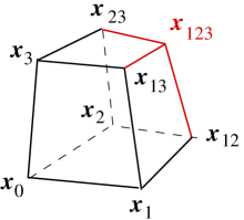
Figure 1. The geometric integrability scheme

Consider points $x_{0}$, $x_{1}$, $x_{2}$ and $x_{3}$ in general position in ${\mathbb{P}}^{M}$, $M\geq 3$. On the plane $\langle x_{0},x_{i},x_{j}\rangle$, $1\leq i<j\leq 3$ choose a point $x_{ij}$ not on the lines $\langle x_{0},x_{i}\rangle$, $\langle x_{0},x_{j}\rangle$ and $\langle x_{i},x_{j}\rangle$. Then there exists the unique point $x_{123}$ which belongs simultaneously to the three planes $\langle x_{3},x_{13},x_{23}\rangle$, $\langle x_{2},x_{12},x_{23}\rangle$ and $\langle x_{1},x_{12},x_{13}\rangle$.

This construction scheme is multidimensionally compatible [35] and provides initial boundary value problem for the corresponding discrete Darboux equations in terms of $K(K-1)$ functions of two discrete variables (implying also multidimensional compatibility of the system). As it was shown in [40], the Darboux transformations of the quadrilateral lattice (thus also the corresponding Bäcklund transformations of the discrete Darboux equations), being discrete symmetries of the quadrilateral lattice Darboux system, can be considered as recursive augmentation of the number of independent variables. Moreover the Bianchi permutability principle of superposition of the transformations, which is often considered as synonymous to integrability, is a consequence of that simple geometric scheme. Therefore the ”compatibility of the construction for arbitrary dimension of the lattice” [35] provides its own commuting symmetries.

We remark that the discrete Darboux equations have been constructed in [16] as the most general discrete system integrable by the nonlocal $\bar{\partial}$–dressing method. Moreover the differential Darboux equations [22] give in a special limit [18] the KP hierarchy of equations (in this context the possibility of considering arbitrary number of independent variables is crucial). This places the quadrilateral lattice (Darboux) equations in a distinguished position among all integrable discrete systems; see also works [17, 41, 39] on the relation of Darboux equations, conjugate nets and quadrilateral lattices, and the multicomponent KP hierarchy [24], which is often considered as the master integrable system.

Having recognized the role of the quadrilateral lattice as the master geometric object of the integrability theory the remaining task is to study integrable reductions of the lattice. If a geometric constraint, imposed on the initial points, propagates during the construction, the corresponding reduction of the discrete Darboux equations is called geometrically integrable. Notice that such consistency of the geometric integrability scheme with the reduction in conjunction with the multidimensional compatibility of the quadrilateral lattice implies the multidimensional compatibility of the reduction. This point of view was used in [19, 28, 36, 32, 33], see also recent review [37], to select integrable reductions of the quadrilateral lattice and to find the corresponding reductions of the discrete Darboux equations.

For example, the integrability of quadrilateral lattices with elementary quadrilaterals inscribed in circles, introduced in [11] as discrete analog of orthogonal coordinate systems, was first proved in this way in [19]. The integrability of the circular lattice was then confirmed by the nonlocal $\bar{\partial}$-dressing method [38], by construction of the corresponding Darboux-type transformation [55] which satisfies [62, 28] the permutability property, by construction of such lattices using the Miwa transformation from the multicomponent BKP hierarchy [39], and by application of the algebro-geometric techniques [4]. Remarkably, as described in [6], there exists a quantization procedure for circular lattices, which leads to solutions of the tetrahedron equation (the three dimensional analog of the Yang–Baxter equation).

In [3] (see also [66]), the notion of multidimensional consistency as a tool to detect integrable equations has been given in the following form: a $d$–dimensional discrete equation possesses the consistency property, if it may be imposed in a consistent way on all $d$–dimensional sublattices of a $(d+1)$–dimensional lattice. In the terminology of [3] the linear problem of the quadrilateral lattice is three–dimensionally consistent, while the discrete Darboux system is four–dimensionally consistent.

It turns out that the geometric notion of integrability of reductions of the quadrilateral lattice very often associates them with classical theorems [21] of incidence geometry. For example, integrability of the circular lattice is a consequence of the Miquel theorem [63]. This observation makes the relation between integrability of the discrete systems and geometry even more profound then the corresponding relation on the level of differential equations. Integrable reductions of the quadrilateral lattice come from two sources. The first are inner (i.e. invariant with respect to the full group of projective transformations of the ambient space) symmetries of the lattice. The second type of reductions arises from the postulated existence of additional structures (e.g., distinguished quadrics, hyperplanes) in the ambient space and mimics the Cayley–Klein approach to subgeometries of the projective geometry, which was the starting point of the famous Erlangen program. Such approach to possible classification of integrable discrete systems was formulated in [28, 29], see also [14, 15].

Apart from the geometric interpretation of the three dimensional Hirota–Miwa equation in its two dimensional Toda lattice form, there is known in the literature [56] an interpretation of its Schwarzian form, the so called Menelaus lattice. It is related to the adjoint linear problem of (1.2) for a map $\boldsymbol{\phi}^{*}:{\mathbb{Z}}^{3}\to{\mathbb{R}}^{M}$ in the affine gauge, and gives the so called discrete Schwarzian KP equation, which is related to the Hirota–Miwa equation by a nonlocal transformation [56, 78, 51]; see also Section 3.

Figure 2. Geometric equivalence of the Laplace sequence $\psi^{\ell}$ of two dimensional quadrilateral lattices, the Menelaus lattice $\phi^{*}$, and three dimensional Desargues lattice $\phi$.

An important observation [10], which was one of motivations of the present research, associates the four dimensional consistency of the discrete Schwarzian KP equation with the Desargues configuration; see Section 2. Another fact, which was the starting point of the paper, is that there is no essential difference between the space of the algebro-geometric solutions of the Hirota–Miwa equations [59, 60] and the quadrilateral lattice Darboux system [4], provided one takes their Laplace transforms [40] into consideration [30].

In the paper we study the maps $\phi:{\mathbb{Z}}^{N}\to{\mathbb{P}}^{M}$ defined by the most simple nontrivial linear condition stating that for any pair of indices $i\neq j$ the points $\phi$, $\phi_{(i)}$ and $\phi_{(j)}$ are collinear. This is a natural geometric counterpart of the linear problem (1.2). We show in a synthetic geometry way that the multidimensional compatibility of the map follows from the Desargues theorem and its higher-dimensional analogs.

Then, in Section 3 we draw algebraic consequences of the geometric definition of the Desargues maps. As the algebraic significance of the Desargues theorem suggest [9], we consider projective spaces over division rings, what leads to the non-Abelian Hirota–Miwa system [68]. We discuss also various gauge-equivalent forms of the equation in the non-commutative setting.

It can be seen both from simple geometric and algebraic considerations that the Desargues maps can be called also multidimensional adjoint Menelaus maps; see Figure 2. We prefer however to call it in a way which reflects the projective geometric character of the lattice and captures simultaneously its integrability properties.

In Section 4 we apply the nonlocal $\bar{\partial}$-dressing method [1, 89, 53] to find large classes of solutions to the Hirota–Miwa system over the field ${\mathbb{C}}$ of complex numbers. In particular we show, as one may expect from works [70, 72, 81, 31], that the $\tau$-function of the Hirota–Miwa system can be identified with the Fredholm determinant of the integral equation inverting the nonlocal $\bar{\partial}$-dressing problem. We find that also on the level of the nonlocal $\bar{\partial}$-dressing method the solution space of the Hirota–Miwa system is the same like in the case of quadrilateral lattice Darboux system [16] provided one takes [40] also the Laplace transformations of the lattice into consideration.

The three point condition in definition of the Desargues map can be considered as a serious degeneration of the quadrilateral lattice map four point condition. Such approach was presented for the three point linear problem of the Menelaus lattice for example in [56]. In Section 5 we show however that the quadrilateral lattice theory and the Desargues lattice theory are equivalent.

After submitting the first version of the manuscript I have learnt on related recent works of W. K. Schief [79] and V. E. Adler [2].

2. Geometry of the Desargues maps

In this Section we study in detail geometric properties of the Desargues maps. After collecting basic facts on the Desargues configuration we state some genericity assumptions concerning the maps. Then we study multidimensional compatibility of the Desargues maps. Here we understand this notion as a possibility of recursive augmentation of the number of independent variables preserving the geometric condition that characterizes the maps. This point of view mimics successive application of the Darboux transformations or the recursion operator [69]. We postpone discussion of the initial boundary value problem for the Desargues maps to Section 5 after we show their relation to the quadrilateral lattices.

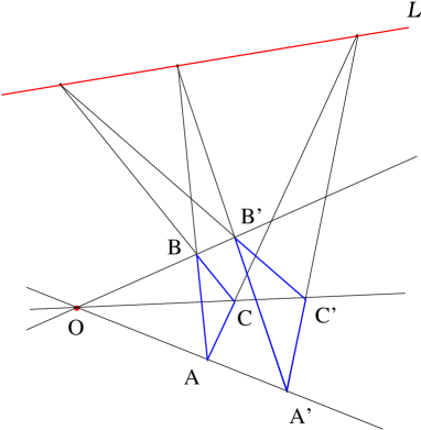
Figure 3. The triangles $\triangle ABC$ and $\triangle A^{\prime}B^{\prime}C^{\prime}$ are perspective from the point $O$ if and only if they are perspective from the line $L$.

2.1. The Desargues configuration

Among all incidence theorems in projective geometry the Desargues theorem (see Figure 3) plays a very distinguished role [21, 9]. It holds in projective spaces of dimension more then two, and is an important element in proving the possibility of introduction of homogeneous coordinates taking values in a division ring; in order to introduce such coordinates on projective planes one should add it as an axiom.

The ten lines involved and the ten points involved are so arranged that each of the ten lines passes through three of the ten points, and each of the ten points lies on three of the ten lines. Under the standard duality of plane projective geometry (where points correspond to lines and collinearity of points corresponds to concurrency of lines), the Desargues configuration is self-dual: axial perspectivity is translated into central perspectivity and vice versa.

At first sight it seems that the Desargues configuration has less symmetry than it really has. However, any of the ten points may be chosen to be the center of perspectivity, and that choice determines which six points will be vertices of triangles and which line will be the axis of perspectivity. The Desargues configuration has symmetry group $S_{5}$ of order $120$. It can be constructed from a $5$ point set, preserving the action of the symmetric group, by letting the points and lines of the Desargues configuration correspond to $2$ and $3$ element subsets of the $5$ points, with incidence corresponding to containment.

Remark.

In the above interpretation of the symmetry group of the Desargues configuration, the $4$ element subsets give rise to $5$ complete quadrilaterals described by the Menelaus theorem, as used in [10] in connection with the four dimensional consistency of the discrete Schwarzian KP equation.

2.2. The Desargues maps

In the paper we study the following maps, the connection of which with the Desargues theorem is essential in showing their multidimensional compatibility.

Definition 2.1.

By Desargues map we mean a map $\phi:{\mathbb{Z}}^{N}\to{\mathbb{P}}^{M}$ of multidimensional integer lattice in Desarguesian projective space of dimension $M\geq 2$, such that for any pair of indices $i\neq j$ the points $\phi$, $\phi_{(i)}$ and $\phi_{(j)}$ are collinear.

Remark.

Notice that we consider ${\mathbb{Z}}^{N}$ as a directed graph.

Remark.

The image of a Desargues map can be called a Desargues lattice. However we would like to stress that we do not use this notion in the sense of the lattice theory as described in [8, 49].

Let us discuss various genericity assumptions of the map. Consider an $N$-dimensional, $N>0$, hypercube graph with a distinguished vertex labeled by ${\emptyset}$, its first order neighbours labeled by ${\{i\}}$, $i=1,\dots,N$, and other vertices labeled as follows: the fourth vertex of a quadrilateral with three other vertices ${I}$, ${I\cup\{i\}}$, ${I\cup\{j\}}$, $i,j\not\in I$, $i\not=j$ is ${I\cup\{i,j\}}$.

Definition 2.2.

A Desargues $N$-hypercube consists of labelled vertices $\phi_{I}$ of an $N$ dimensional hypercube in projective space ${\mathbb{P}}^{M}$, $M\geq 2$, such that for arbitrary multiindex $I\varsubsetneq\{1,2,\dots,N\}$ there exists a line $L_{I}$ incident with $\phi_{I}$ and with all the points $\phi_{I\cup\{i\}}$, $i\notin I$. A Desargues $N$-hypercube is called non-degenerate if all its vertices are distinct. A non-degenerate Desargues $N$-hypercube is called weakly generic if all the lines $L_{I}$ are distinct.

Given two multiindices $I_{1},I_{2}$, with $I_{1}\subset I_{2}$, the points $\phi_{J}$, $I_{1}\subset J\subset I_{2}$, of a weakly generic Desargues $N$-hypercube form weakly generic Desargues $(|I_{2}|-|I_{1}|)$-hypercube. The space $\pi_{I_{1},I_{2}}$ spanned by the points $\phi_{J}$, $I_{1}\subset J\subset I_{2}$, has dimension $(|I_{2}|-|I_{1}|)$ at most. For example, $L_{I}=\pi_{I,I\cup\{i\}}$ for all $i\notin I$. We write also $\pi_{I}=\pi_{\emptyset,I}$.

Definition 2.3.

A Desargues $N$-hypercube is called generic if $\dim\pi_{I_{1},I_{2}}=|I_{2}|-|I_{1}|$ for all $I_{1}\subset I_{2}$.

Remark.

Notice that suitable projections of a generic Desargues hypercubes can produce weakly generic Desargues hypercubes.

Definition 2.4.

A Desargues map $\phi:{\mathbb{Z}}^{N}\to{\mathbb{P}}^{M}$ is called (weakly) generic if the corresponding Desargues lattice consists of (weakly) generic Desargues $N$-hypercubes under identification $\phi_{I}$ with $\phi_{(I)}$ for a fixed point $\phi$ of the lattice.

Notice that any weakly generic Desargues map $\phi:{\mathbb{Z}}^{N}\to{\mathbb{P}}^{M}$ induces a map $L:{\mathbb{Z}}^{N}\to{\mathbb{G}}^{M}_{1}$ into the Grassmann space of lines in ${\mathbb{P}}^{M}$, where $L$ is the line coincident with the point $\phi$ and all the neighbouring $\phi_{(i)}$, $i=1,\dots,N$. Such maps are characterized by the following two properties.
(i) Any two neighbouring lines $L$ and $L_{(i)}$ intersect.
(ii) The intersection points $L\cap L_{(-i)}$ coincide for all $1\leq i\leq N$.

The maps $L:{\mathbb{Z}}^{N}\to{\mathbb{G}}^{M}_{1}$ satisfying the first condition only, play an important role in the theory of Darboux transformations of the quadrilateral lattice [40] and are called line congruences. It is natural to call the line congruences satisfying also the second condition the Desargues congruences. Then the points of the Desargues lattice can be recovered by $\phi=L\cap L_{(-i)}$, $i=1,\dots,N$.

2.3. Multidimensional compatibility of Desargues maps

Given point $\phi$ and its two nearest (in positive directions) neighbours $\phi_{(i)}$ and $\phi_{(j)}$. By definition there exists a line $L$ incident with the three points. Assuming the Desargues map is weakly generic, the point $\phi_{(ij)}$ can be an arbitrary point not on the line $L$. Such a choice determines the lines $L_{(i)}$ and $L_{(j)}$.

2.3.1. Three dimensional compatibility and the Veblen–Young axiom

Consider a point $\phi_{(k)}\in L$, $k\neq i,j$. On the line $L_{(i)}$ choose a point $\phi_{(ik)}$ distinct from $\phi_{(i)}$ and $\phi_{(ij)}$, thus determining the line $L_{(k)}$. Then three dimensional compatibility of the Desargues map, i.e. the existence of the intersection point $\phi_{(jk)}$ of lines $L_{(j)}$ and $L_{(k)}$, is equivalent to the Veblen-Young axiom of the synthetic projective geometry, which in the current notation states (compare Figure 2).

Given four distinct points $\phi_{(j)}$, $\phi_{(k)}$, $\phi_{(ij)}$, $\phi_{(ik)}$; if the lines $L_{\phi_{(j)}\phi_{(k)}}=L$ and $L_{\phi_{(ij)}\phi_{(ik)}}=L_{(i)}$ intersect, then the lines $L_{\phi_{(j)}\phi_{(ij)}}=L_{(j)}$ and $L_{\phi_{(k)}\phi_{(ik)}}=L_{(k)}$ intersect as well.

There is no condition for the point $\phi_{(ijk)}$, apart from weak genericity assumption, which means that it should not be placed on the lines $L$, $L_{(i)}$, $L_{(j)}$, $L_{(k)}$.

2.3.2. Four dimensional compatibility and the Desargues theorem

Add the next point $\phi_{(\ell)}$ on the line $L$, $\ell\neq i,j,k$, and the point $\phi_{(i\ell)}\in L_{(i)}$. The corresponding line $L_{(\ell)}$, incident with $\phi_{(\ell)}$ and $\phi_{(i\ell)}$, intersects (by Veblen–Young) the lines $L_{(j)}$, $L_{(k)}$ in the points $\phi_{(j\ell)}$ and $\phi_{(k\ell)}$, correspondingly. The problem is to find the four points $\phi_{(ijk)}$, $\phi_{(ij\ell)}$, $\phi_{(ik\ell)}$ and $\phi_{(jk\ell)}$ which satisfy the Desargues map condition.

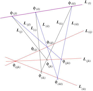
Figure 4. The four dimensional compatibility of the Desargues map

Choose a point $\phi_{(ij\ell)}$, not on the lines $L$, $L_{(i)}$, $L_{(j)}$, $L_{(k)}$, and define therefore the lines $L_{(ij)}$, $L_{(i\ell)}$ and $L_{(j\ell)}$. On the line $L_{(i\ell)}$ mark a point $\phi_{(ik\ell)}$, thus defining the lines $L_{(ik)}$ and $L_{(k\ell)}$. The lines $L_{(j\ell)}$ and $L_{(k\ell)}$ intersect (by Veblen–Young) in the point $\phi_{(jk\ell)}$, which gives the line $L_{(jk)}$. We have constructed two triangles in perspective from the line $L_{(\ell)}$: the first with vertices $\phi_{(ij)}$, $\phi_{(ik)}$, $\phi_{(jk)}$, and the second with vertices $\phi_{(ij\ell)}$, $\phi_{(ik\ell)}$, $\phi_{(jk\ell)}$. By the Desargues theorem the three lines $L_{(ij)}$, $L_{(ik)}$ and $L_{(jk)}$ intersect in one point, which is by construction $\phi_{(ijk)}$.

Remark.

Notice that in the generic case when the points $\phi$, $\phi_{(i)}$, $\phi_{(ij)}$ and $\phi_{(ijk)}$ generate the space $\pi_{(ijk)}$ of dimension three, then all the points whose shifts contain the index $\ell$ are obtained as intersections of the lines of the ”$ijk$ configuration” with the plane generated by the points $\phi_{(\ell)}$, $\phi_{(i\ell)}$ and $\phi_{(ij\ell)}$. Moreover, to keep the configuration generic we add the point $\phi_{(ijk\ell)}$ (which is not specified by the previous construction) outside the space $\pi_{(ijk)}$ thus generating the four dimensional space $\pi_{(ijk\ell)}$.

2.3.3. The multidimensional compatibility for arbitrary $N$

The multidimensional compatibility of the Desargues map is equivalent to existence of a Desargues $N$-hypercube for arbitrary $N$, provided appropriate initial data have been prescribed. The following proposition allows to construct generic Desargues $(N+1)$-hypercubes from generic Desargues $N$-hypercubes in spaces of the dimension large enough. It is an analogue of the well known, mentioned in the Remark above, three dimensional proof of the Desargues theorem. By suitable projections one can produce therefore weakly generic Desargues hypercubes.

Proposition 2.1.

Given generic Desargues $N$-hypercube in ${\mathbb{P}}^{M}$, where $N<M$. On the $N$ lines $L_{\emptyset}$, $L_{\{1\}}$, $L_{\{1,2\}}$, $L_{\{1,2,\dots,N-1\}}$, chose $N$ points $\phi_{\{N+1\}}$, $\phi_{\{1,N+1\}}$, $\phi_{\{1,2,N+1\}}$, …$\phi_{\{1,2,\dots,N-1,N+1\}}$ in generic position, correspondingly, in such a way that the $N-1$ dimensional subspace $U$ of $\pi_{\{1,2,\dots,N\}}$

$$U=\langle\phi_{\{N+1\}},\phi_{\{1,N+1\}},\phi_{\{1,2,N+1\}},\dots\phi_{\{1,2,\dots,N-1,N+1\}}\rangle$$

is not incident with any vertex of the hypercube. Then the unique intersection points $\phi_{\{I,N+1\}}=U\cap L_{I}$ of the hyperplane with the lines of the $N$-hypercube, and the points of the initial hypercube supplemented by a point $\phi_{\{1,2,\dots,N,N+1\}}\notin\pi_{\{1,2,\dots,N\}}$ give a generic Desargues $(N+1)$-hypercube.

Proof.

By the assumption of the Proposition the lines $L_{I}$, $I\varsubsetneq\{1,2,\dots,N\}$, are not contained in the hyperplane $U$, thus all the points $\phi_{I\cup\{N+1\}}$ are well defined. Having then all the vertices of the $(N+1)$-hypercube we will check that it satisfies the desired properties.

Given multiindex $I\varsubsetneq\{1,2,\dots,N,N+1\}$ there are two possibilities.
(i) $N+1\notin I$. When $|I|=N$ then $I=\{1,2,\dots,N\}$ and define $L_{I}$ as the unique line incident with $\phi_{\{1,2,\dots,N\}}$ and $\phi_{\{1,2,\dots,N,N+1\}}$. If $|I|<N$ then take as the line $L_{I}$ the line of the $N$-hypercube, and $\phi_{I\cup\{N+1\}}\in L_{I}$ by construction.
(ii) $N+1\in I$. There exists $i\in\{1,2,\dots,N\}$, $i\notin I$. Set $L_{I}$ as the unique line incident with $\phi_{I}$ and $\phi_{I\cup\{i\}}$. To conclude the proof of the Desargues property we will show that $L_{I}$ is independent of a particular choice of such an index $i$. When $|I|=N$ then there is nothing to prove because there is only one index $i\notin I$. If $1\leq|I|<N$ set $J=I\setminus\{N+1\}$, there exists $j\in\{1,2,\dots,N\}$, $i\not=j$, and $j\notin J$. Consider the plane $\pi_{J,J\cup\{i,j\}}$ which contains the three lines $L_{J}$, $L_{J\cup\{i\}}$ and $L_{J\cup\{j\}}$, and is not contained in $U$. Then $L_{I}=\pi_{J,J\cup\{i,j\}}\cap U$ which shows that also $\phi_{J\cup\{j,N+1\}}=\phi_{I\cup\{j\}}\in L_{I}$, thus also the index $j$ can be used to define $L_{I}$.

Finally, to prove genericity of the Desargues $(N+1)$-hypercube notice that for all $I_{1}\subset I_{2}\subset\{1,2,\dots,N\}$ the intersection $\pi_{I_{1},I_{2}}\cap L_{I_{2}}$ is the point $\phi_{I_{2}}$ only. This implies that $\dim\pi_{I_{1}\cup\{N+1\},I_{2}\cup\{N+1\}}=|I_{2}|-|I_{1}|$, and $\dim\pi_{I_{1},I_{2}\cup\{N+1\}}=|I_{2}|-|I_{1}|+1$. ∎

2.4. The adjoint Desargues maps

To obtain the analogous geometric meaning of the adjoint of the linear problem of the Hirota–Miwa system, define the adjoint Desargues maps (or multidimensional Menelaus maps, if one restricts to affine part of ${\mathbb{P}}^{M}$) as maps $\phi^{*}:{\mathbb{Z}}^{N}\to{\mathbb{P}}^{M}$ such that for any pair of indices $i\neq j$ the points $\phi^{*}_{(i)}$, $\phi^{*}_{(j)}$ and $\phi^{*}_{(ij)}$ are collinear. This leads to the following definition of an adjoint Desargues $N$-hypercube.

Definition 2.5.

An adjoint Desargues $N$-hypercube consists of labelled vertices of an $N$ dimensional hypercube in projective space ${\mathbb{P}}^{M}$, $M\geq 2$, such that for arbitrary multiindex $I\subset\{1,2,\dots,N\}$, $|I|>1$, and for any pair of distinct indices $i,j\in I$ the vertex $\phi^{*}_{I}$ is incident with a line passing through $\phi^{*}_{I\setminus\{i\}}$ and $\phi^{*}_{I\setminus\{j\}}$.

One can notice that given Desargues map $\phi:{\mathbb{Z}}^{N}\to{\mathbb{P}}^{M}$, its superposition $\phi\circ\imath$ with the arrows inversion map $\imath:{\mathbb{Z}}^{N}\to{\mathbb{Z}}^{N}$, $\imath(n)=-n$, is an adjoint Desargues map (and vice versa). Similarly, any Desargues $N$-hypercube gives rise to the adjoint Desargues $N$-hypercube under identification $\phi^{*}_{I}=\phi_{\{1,2,\dots,N\}\setminus I}$. The geometric theory of the adjoint Desargues map follows from that identification.

3. Desargues maps and various non-commutative discrete KP equations

In this Section we study algebraic consequences of the geometric definition of the Desargues map $\phi:{\mathbb{Z}}^{N}\to{\mathbb{P}}^{M}$. Because to prove its multidimensional compatibility we use only the Desargues theorem then the natural coordinates of the projective space are elements of a division ring ${\mathbb{D}}$. This leads to the corresponding non-commutative nonlinear equations which we formulate first in arbitrary gauge, i.e., keeping the freedom in rescaling the homogeneous coordinates by a nonzero factor. Two basic specifications of the gauge are discussed in the second part of this Section.

3.1. The linear problem for the Desargues maps and its compatibility conditions

In the homogeneous coordinates $\boldsymbol{\phi}:{\mathbb{Z}}^{N}\to{\mathbb{D}}^{M+1}_{*}$ (we consider right vector spaces) the map can be described in terms of the linear system

(3.1) $$\boldsymbol{\phi}+\boldsymbol{\phi}_{(i)}A_{ij}+\boldsymbol{\phi}_{(j)}A_{ji}=0,\qquad i\neq j,$$

where $A_{ij}:{\mathbb{Z}}^{N}\to{\mathbb{D}}_{*}$ are certain non-vanishing functions.

Proposition 3.1.

The compatibility of the linear system (3.1) is equivalent to equations

(3.2) $$A_{ij}^{-1}A_{ik}+A_{kj}^{-1}A_{ki}=1,$$

(3.3) $$A_{ik(j)}A_{jk}=A_{jk(i)}A_{ik},$$

where the indices $i,j,k$ are distinct.

Proof.

From the linear problem (3.1) for the pair $(i,k)$ find $\boldsymbol{\phi}_{(k)}$ in terms of $\boldsymbol{\phi}$ and $\boldsymbol{\phi}_{(i)}$. Similarly, find $\boldsymbol{\phi}_{(k)}$ from the equation for the pair $(j,k)$. Comparing the resulting relation between $\boldsymbol{\phi}$ and $\boldsymbol{\phi}_{(i)}$ and $\boldsymbol{\phi}_{(j)}$ with the linear problem (3.1) for the pair $(i,j)$ gives, after some elementary algebra, the first equation.

The compatibility of the linear problem (3.1) shifted in $k$ direction with two other similar equations involving three distinct indices $i,j,k$ gives rise to a linear relation between $\boldsymbol{\phi}$, $\boldsymbol{\phi}_{(k)}$ and $\boldsymbol{\phi}_{(ij)}$. Their linear independence implies the vanishing of the corresponding coefficients

(3.4) $$A_{ik}^{-1}A_{kj(i)}^{-1}A_{ij(k)}+A_{jk}^{-1}A_{ki(j)}^{-1}A_{ji(k)} =0,$$

(3.5) $$1+A_{ki}A_{ik}^{-1}A_{kj(i)}^{-1}A_{ij(k)}+A_{kj}A_{jk}^{-1}A_{ki(j)}^{-1}A_{ji(k)} =0,$$

(3.6) $$A_{jk(i)}A_{kj(i)}^{-1}A_{ij(k)}+A_{ik(j)}A_{ki(j)}^{-1}A_{ji(k)} =0.$$

Equations (3.4) and (3.6) directly lead (3.3).

Using (3.3) we can replace equations (3.4) and (3.5) by

(3.7) $$A_{ik}^{-1}A_{ij}A_{kj}^{-1}+A_{jk}^{-1}A_{ji}A_{ki}^{-1} =0,$$

(3.8) $$1+(A_{ki}-A_{kj})A_{ik}^{-1}A_{ij}A_{kj}^{-1} =0.$$

We will show that equation (3.7) follows from the condition (3.2). Indeed, starting from the identity

$$A_{kj}(1-A_{kj}^{-1}A_{ki})+A_{ki}(1-A_{ki}^{-1}A_{kj})=0,$$

and using (3.2) we get

$$A_{kj}A_{ij}^{-1}A_{ik}+A_{ki}A_{ji}^{-1}A_{jk}=0,$$

equivalent to (3.7). Also equation (3.8) is a direct consequence of the condition (3.2). ∎

Corollary 3.2.

For any three distinct indices $i,j,k$ we can write down three distinct equations of the form (3.2). However any two of them imply the third one.

Proof.

Equation (3.2), where the indices $i$ and $k$ enter symmetrically is equivalent to

(3.9) $$A_{ki}^{-1}A_{kj}=\left(1-A_{ij}^{-1}A_{ik}\right)^{-1}.$$

Adding equation (3.9) to the similar one with the indices $k$ and $j$ exchanged one obtains equation (3.2) with the indices $i$ and $j$ exchanged

$$A_{ji}^{-1}A_{jk}+A_{ki}^{-1}A_{kj}=\left[A_{ik}^{-1}\left(A_{ik}-A_{ij}\right)\right]^{-1}+\left[A_{ij}^{-1}\left(A_{ij}-A_{ik}\right)\right]^{-1}=\left(A_{ij}-A_{ik}\right)^{-1}\left(A_{ij}-A_{ik}\right)=1.$$

∎

Corollary 3.3.

Equations (3.3) imply existence of the potentials $\rho_{i}:{\mathbb{Z}}^{N}\to{\mathbb{D}}_{*}$, unique up to functions of single variables $n_{i}$, such that

(3.10) $$\rho_{i(j)}=A_{ji}\rho_{i},\qquad i\neq j.$$

3.2. Gauges

We are still left with the possibility to apply the gauge transformation

(3.11) $$\boldsymbol{\phi}=\tilde{\boldsymbol{\phi}}G,$$

where $G:{\mathbb{Z}}^{N}\to{\mathbb{D}}_{*}$ is an arbitrary non-vanishing function. Then $\tilde{\boldsymbol{\phi}}$ satisfies the linear problem (3.1) with the coefficients

(3.12) $$\tilde{A}_{ij}=G_{(i)}A_{ij}G^{-1}.$$

By fixing properties of $G$ one can arrive to relation between the coefficients of the linear problem. We will discuss two gauges. First gauge, which because of the geometric interpretation can be called the affine gauge, gives in the commutative case the discrete modified KP system. The second gauge in the commutative case leads to the Hirota–Miwa system.

3.2.1. The modified discrete KP gauge

Proposition 3.4.

When the gauge function is a non-vanishing solution of the linear problem (3.1) then the coefficients $\tilde{A}_{ij}$ are constrained by the relation

(3.13) $$\tilde{A}_{ij}+\tilde{A}_{ji}=-1,\qquad i\neq j.$$

Remark.

When as the solution of the linear problem is taken the last coordinate $\phi^{M+1}$ of the homogeneous representation of the map then we obtain the standard transition to the non-homogeneous coordinates.

Remark.

In the affine gauge the algebraic compatibility system (3.2) consists, for any triple of distinct indices $i,j,k$, of one independent equation.

It is convenient (we follow the reasoning presented in [78] in the commutative case) to rewrite the linear problem (3.1) subject to condition (3.13) as

(3.14) $$(\boldsymbol{\phi}_{(j)}-\boldsymbol{\phi})=(\boldsymbol{\phi}_{(i)}-\boldsymbol{\phi})B_{ij},$$

where

(3.15) $$B_{ij}=B_{ji}^{-1}=A_{ij}(1+A_{ij})^{-1}.$$

Then the algebraic compatibility takes the form

(3.16) $$B_{ij}B_{jk}=B_{ik},$$

which allows for introduction of a potential $\sigma:{\mathbb{Z}}^{N}\to{\mathbb{D}}_{*}$ such that

(3.17) $$B_{ij}=\sigma_{(i)}\sigma_{(j)}^{-1}.$$

The second part of the compatibility condition takes then the form of the non-commutative discrete mKP system [67]

(3.18) $$(\sigma_{(i)}^{-1}-\sigma_{(j)}^{-1})\sigma_{(ij)}+(\sigma_{(j)}^{-1}-\sigma_{(k)}^{-1})\sigma_{(jk)}+(\sigma_{(k)}^{-1}-\sigma_{(i)}^{-1})\sigma_{(ki)}=0.$$

Finally, notice that due to the compatibility of the system

(3.19) $$(\boldsymbol{\phi}_{(j)}-\boldsymbol{\phi})\sigma_{(j)}=(\boldsymbol{\phi}_{(i)}-\boldsymbol{\phi})\sigma_{(i)},$$

each coordinate $\phi^{k}:{\mathbb{Z}}^{N}\to{\mathbb{D}}$ of $\boldsymbol{\phi}$ satisfies the generalized lattice spin system [67]

(3.20) $$(\phi_{(jk)}-\phi_{(k)})(\phi_{(jk)}-\phi_{(j)})^{-1}(\phi_{(ij)}-\phi_{(j)})(\phi_{(ij)}-\phi_{(i)})^{-1}(\phi_{(ik)}-\phi_{(i)})(\phi_{(ik)}-\phi_{(k)})^{-1}=1,$$

called also the non-commutative Schwarzian discrete KP system [17, 57].

3.2.2. The Hirota–Miwa system gauge

In order to introduce the second gauge we need the following result.

Lemma 3.5.

There exists non-vanishing function $G$ defined as a solution of the system

(3.21) $$G_{(i)}A_{ij}=-G_{(j)}A_{ji},\qquad i\neq j.$$

Proof.

The algebraic compatibility of equations (3.21) for three pairs of indices $i,j,k$, has the form

(3.22) $$A_{jk}^{-1}A_{ji}A_{ij}^{-1}+A_{kj}^{-1}A_{ki}A_{ik}^{-1}=0,\qquad i,j,k\quad\text{distinct}.$$

It can be proved by application of the algebraic compatibility condition (3.2) starting from the identity

$$(1-A_{ik}^{-1}A_{ij})A_{ij}^{-1}+(1-A_{ij}^{-1}A_{ik})A_{ik}^{-1}=0.$$

∎

Proposition 3.6.

The linear system (3.1) is gauge equivalent to the discrete linear problem of the non-Abelian Hirota–Miwa system [25, 68]

(3.23) $$\boldsymbol{\phi}_{(i)}-\boldsymbol{\phi}_{(j)}=\boldsymbol{\phi}U_{ij},\qquad i\neq j\leq N.$$

Proof.

Take the gauge function $G$ as in Lemma above, which gives (we skip tildes)

(3.24) $$A_{ij}=-A_{ji},$$

and set $U_{ij}=A_{ji}^{-1}$. ∎

In this gauge the compatibility conditions (3.2)-(3.3) reduce to the following systems for distinct triples $i,j,k$

(3.25) $$U_{ij}+U_{jk}+U_{ki}=0,$$

(3.26) $$U_{kj}U_{ki(j)}=U_{ki}U_{kj(i)}.$$

This allows to introduce potentials $r_{i}:{\mathbb{Z}}^{N}\to{\mathbb{D}}_{*}$ such that

(3.27) $$r_{i(j)}=r_{i}U_{ij},\qquad i\neq j;$$

see [68] for further properties of the system.

Remark.

In the commutative case the functions $r_{i}$ can be parametrized in terms of a single potential $\tau$

(3.28) $$r_{i}=(-1)^{\sum_{k<i}n_{k}}\frac{\tau_{(i)}}{\tau},$$

which leads to the linear problem (1.2), while and the algebraic compatibility (3.25) gives the Hirota–Miwa system (1.1).

4. Application of the nonlocal $\bar{\partial}$-dressing method

In this Section the division ring ${\mathbb{D}}$ is replaced by the field ${\mathbb{C}}$ of complex numbers. By application of the nonlocal $\bar{\partial}$-dressing method [1, 89, 53] we construct solutions of the Hirota–Miwa system and the corresponding solutions of the linear problem.

Consider the following integro-differential equation in the complex plane ${\mathbb{C}}$

(4.1) $$\bar{\partial}\chi(\lambda)=\bar{\partial}\eta(\lambda)+\int_{\mathbb{C}}R(\lambda,\lambda^{\prime})\chi(\lambda^{\prime})\>d\lambda^{\prime}\wedge d\bar{\lambda}^{\prime},$$

where $R(\lambda,\lambda^{\prime})$ is a given $\bar{\partial}$ datum, which decreases quickly enough at $\infty$ in $\lambda$ and $\lambda^{\prime}$, and the function $\eta(\lambda)$, the normalization of the unknown $\chi(\lambda)$, is a given rational function, which describes the polar behavior of $\chi(\lambda)$ in ${\mathbb{C}}$ and its behavior at $\infty$:

$$\chi(\lambda)-\eta(\lambda)\to 0,\qquad\text{for}\quad|\lambda|\to\infty.$$

We remark that the dependence of $\chi(\lambda)$ and $R(\lambda,\lambda^{\prime})$ on $\bar{\lambda}$ and $\bar{\lambda}^{\prime}$ will be systematically omitted, for notational convenience.

Due to the generalized Cauchy formula the nonlocal $\bar{\partial}$ problem (4.1) is equivalent to the following Fredholm integral equation of the second kind

(4.2) $$\chi(\lambda)=\eta(\lambda)-\int_{\mathbb{C}}K(\lambda,\lambda^{\prime})\chi(\lambda^{\prime})d\lambda^{\prime}\wedge d\bar{\lambda}^{\prime},$$

with the kernel

(4.3) $$K(\lambda,\lambda^{\prime})=\frac{1}{2\pi i}\int_{\mathbb{C}}\frac{R(\lambda^{\prime\prime},\lambda^{\prime})}{\lambda^{\prime\prime}-\lambda}d\lambda^{\prime\prime}\wedge d\bar{\lambda}^{\prime\prime}.$$

Recall (see, for example [83]) that the Fredholm determinant $D$ is defined by the series

(4.4) $$D=1+\sum_{m=1}^{\infty}\frac{1}{m!}\int_{{\mathbb{C}}^{m}}K\begin{pmatrix}\zeta_{1}&\zeta_{2}&\dots&\zeta_{m}\\ \zeta_{1}&\zeta_{2}&\dots&\zeta_{m}\end{pmatrix}d\zeta_{1}\wedge d\bar{\zeta}_{1}\dots d\zeta_{m}\wedge d\bar{\zeta}_{m}\;,$$

where

$$K\begin{pmatrix}\zeta_{1}&\zeta_{2}&\dots&\zeta_{m}\\ \mu_{1}&\mu_{2}&\dots&\mu_{m}\end{pmatrix}=\det\begin{pmatrix}K(\zeta_{i},\mu_{j})\end{pmatrix}_{1\leq i,j\leq m}.$$

For a non-vanishing Fredholm determinant the solution of (4.2) can be written in the form

(4.5) $$\chi(\lambda)=\eta(\lambda)-\int_{\mathbb{C}}\frac{D(\lambda,\lambda^{\prime})}{D}\eta(\lambda^{\prime})d\lambda^{\prime}\wedge d\bar{\lambda}^{\prime},$$

where the Fredholm minor is defined by the series

(4.6) $$D(\lambda,\lambda^{\prime})=\sum_{m=0}^{\infty}\frac{1}{m!}\int_{{\mathbb{C}}^{m}}K\begin{pmatrix}\lambda&\zeta_{1}&\dots&\zeta_{m}\\ \lambda^{\prime}&\zeta_{1}&\dots&\zeta_{m}\end{pmatrix}d\zeta_{1}\wedge d\bar{\zeta}_{1}\dots d\zeta_{m}\wedge d\bar{\zeta}_{m}\;.$$

Let $\lambda_{i}\in{\mathbb{C}}$, $i=1,\dots,N$ be distinct points of the complex plane. Consider the following dependence of the kernel $R$ on the variables $n=(n_{1},\dots,n_{N})\in{\mathbb{Z}}^{N}$

(4.7) $$R_{(i)}(\lambda,\lambda^{\prime};n)=(\lambda-\lambda_{i})^{-1}R(\lambda,\lambda^{\prime})(\lambda^{\prime}-\lambda_{i}),$$

or equivalently

(4.8) $$R(\lambda,\lambda^{\prime};n)=E(\lambda;n)^{-1}R_{0}(\lambda,\lambda^{\prime})E(\lambda^{\prime};n),\qquad E(\lambda;n)=\prod_{i=1}^{N}(\lambda-\lambda_{i})^{n_{i}},$$

where $R_{0}(\lambda,\lambda^{\prime})$ is independent of $n$. We assume that $R_{0}$ decreases at $\lambda_{i}$ and in poles of the normalization function $\eta$ fast enough such that $\chi-\eta$ is regular in these points [18, 16].

Remark.

In the paper we always assume that the kernel $R$ in the nonlocal $\bar{\partial}$ problem is such that the Fredholm equation (4.2) is uniquely solvable. Then, by the Fredholm alternative, the homogeneous equation with $\eta=0$ has only the trivial solution.

Remark.

The structure of the function $E(\lambda;n)$ mimics the analytic structure of the Baker–Akhezer wave function used in [60] to solve the Hirota–Miwa system by the algebro-geometric techniques, where the role of the Fredholm alternative is played by the Riemann–Roch theorem.

Lemma 4.1.

The evolution (4.9) of the kernel of the Fredholm equation implies the following evolution of the determinants in the series defining the Fredholm determinant $D$

$$K_{(i)}\left(\begin{matrix}\zeta_{1}&\dots&\zeta_{m}\\ \zeta_{1}&\dots&\zeta_{m}\end{matrix}\biggr{\rvert}\;n\right)=K\left(\begin{matrix}\zeta_{1}&\dots&\zeta_{m}\\ \zeta_{1}&\dots&\zeta_{m}\end{matrix}\biggr{\rvert}\;n\right)-\sum_{j=1}^{m}K\left(\begin{matrix}\zeta_{1}&\dots&\lambda_{i}&\dots&\zeta_{m}\\ \zeta_{1}&\dots&\zeta_{j}&\dots&\zeta_{m}\end{matrix}\biggr{\rvert}\;n\right).$$

Proof.

The evolution (4.7) of the kernel $R$ implies that the kernel $K$ of the integral equation (4.2) is subject to the equation

(4.9) $$K_{(i)}(\lambda,\lambda^{\prime};n)=(\lambda-\lambda_{i})^{-1}\left[K(\lambda,\lambda^{\prime};n)-K(\lambda_{i},\lambda^{\prime};n)\right](\lambda^{\prime}-\lambda_{i}),$$

the conclusion is reached by basic linear algebra. ∎

Proposition 4.2.

Let $\chi(\lambda;n)$ be a solution of the $\bar{\partial}$ problem (4.1) with the canonical normalization $\eta=1$ then the function $\psi(\lambda;n)=\chi(\lambda;n)E(\lambda;n)$ satisfies the linear system (3.23) with the potentials

(4.10) $$U_{ij}(n)=(\lambda_{j}-\lambda_{i})\frac{\chi_{(j)}(\lambda_{i};n)}{\chi(\lambda_{i};n)}.$$

Proof.

The combination $(\lambda-\lambda_{i})\chi_{(i)}(\lambda;n)-(\lambda-\lambda_{j})\chi_{(j)}(\lambda;n)$ satisfies the Fredholm equation with constant (in $\lambda$) normalization thus must be proportional to $\chi(\lambda;n)$. By evaluating of both sides in $\lambda_{i}$ we find the coefficient of proportionality. Multiplication of both sides by $E(\lambda;n)$ gives the statement. ∎

Corollary 4.3.

The form of $U_{ij}$ given above implies that the potentials $r_{i}$, defined by equation (3.27), read

(4.11) $$r_{i}(n)=\prod_{k\neq i}(\lambda_{k}-\lambda_{i})^{n_{k}}\chi(\lambda_{i};n).$$

Theorem 4.4.

Within the considered class of solutions of the Hirota–Miwa system the $\tau$-function is given by

(4.12) $$\tau(n)=(-1)^{\sum_{i<j}n_{i}n_{j}/2}\prod_{i\neq j}(\lambda_{i}-\lambda_{j})^{n_{i}n_{j}/2}D(n).$$

Proof.

Evaluation of equation (4.5) at $\lambda_{i}$ for $\chi(\lambda;n)$ like in Proposition 4.2 gives

(4.13) $$\chi(\lambda_{i};n)=1-\int_{\mathbb{C}}\frac{D(\lambda_{i},\lambda^{\prime};n)}{D(n)}d\lambda^{\prime}\wedge d\bar{\lambda}^{\prime}.$$

From Lemma 4.1 we obtain that

(4.14) $$D_{(i)}(n)=D(n)-\int_{\mathbb{C}}D(\lambda_{i},\lambda^{\prime};n)d\lambda^{\prime}\wedge d\bar{\lambda}^{\prime}.$$

Comparison of both equations shows that

(4.15) $$D_{(i)}(n)=\chi(\lambda_{i};n)D(n),$$

which due to equations (3.28) and (4.11) gives the statement. ∎

The above result, provides the ”determinant interpretation” of the $\tau$-function within the class of solutions which can be obtained by application of the nonlocal $\bar{\partial}$-dressing method.

Recently, within the same approach the $\tau$-function of the quadrilateral lattices has been studied [31]. As it can be deduced from [16, 40], the structure of the $\bar{\partial}$ datum in the nonlocal $\bar{\partial}$-dressing method which leads to the quadrilateral lattices and all the lattices generated by their Laplace transforms is as follows. Let $\lambda_{i}^{\pm}\in{\mathbb{C}}$, $i=1,\dots,K$ be pairs of distinct points of the complex plane, let $m=(m_{1},\dots,m_{K})\in{\mathbb{Z}}^{K}$ be points of the ${\mathbb{Z}}^{K}$ integer lattice and let $\ell=(\ell_{1},\dots,\ell_{K})$, $\ell_{1}+\ell_{2}+\dots+\ell_{K}=0$, be a point of the $A_{K-1}$ root lattice. The function $E(\lambda;(m,\ell))$ which should replace the function $E(\lambda;n)$ in equation (4.8) reads

(4.16) $$E(\lambda;(m,\ell))=\prod_{i=1}^{K}\frac{(\lambda-\lambda^{-}_{i})^{m_{i}}}{(\lambda-\lambda^{+}_{i})^{m_{i}+\ell_{i}}}.$$

The variable $m$ is the quadrilateral lattice discrete parameter, while the Laplace transformation ${\mathcal{L}}_{ij}$ is given by $\ell_{i}\mapsto\ell_{i}+1$, $\ell_{j}\mapsto\ell_{j}-1$. After the proper identification of $2K$ points $\lambda_{i}^{\pm}$, $i=1,\dots,K$, with the points $\lambda_{1},\dots,\lambda_{2K-1},\lambda_{2K}=\infty$, we obtain the change of variables discussed in Section 5.

5. Desargues maps and quadrilateral lattices

This Section is devoted to the study of the relation between Desargues maps and quadrilateral lattices. We will show that the theory of quadrilateral lattices can be embedded in the theory the Desargues maps, and for odd $N=2K-1$ this embedding is one-to-one (the case of even $N=2K$ can be treated as dimensional reduction of $2K+1$). The relation described below generalizes the relation, known on the $\tau$-function level, between the Hirota–Miwa equation and its version in the discrete two dimensional Toda lattice form [88]. The relation between discrete two dimensional Toda lattice and two dimensional quadrilateral lattice was the subject of [26, 27].

Recall that the condition of planarity of elementary quadrilaterals of $\psi:{\mathbb{Z}}^{K}\to{\mathbb{P}}^{M}$ written in the non-homogeneous coordinates $\boldsymbol{\psi}:{\mathbb{Z}}^{K}\to{\mathbb{D}}^{M}$ gives the following linear problem

(5.1) $$\boldsymbol{\psi}_{(ij)}-\boldsymbol{\psi}=(\boldsymbol{\psi}_{(i)}-\boldsymbol{\psi})a_{ij}+(\boldsymbol{\psi}_{(j)}-\boldsymbol{\psi})a_{ji},\qquad i\neq j,$$

where $a_{ij}:{\mathbb{Z}}^{K}\to{\mathbb{D}}$ are certain functions which should satisfy the corresponding compatibility condition (a version of the discrete Darboux system).

The Laplace transformation $\mathcal{L}_{ij}$ of $\psi$ is constructed [26, 40] via intersection of the tangent lines $\langle\psi,\psi_{(i)}\rangle$ with their $j$-th negative neighbours $\langle\psi_{(-j)},\psi_{(i,-j)}\rangle$, see Figure 5.

Figure 5. The Laplace transform of the quadrilateral lattice

In the non-homogeneous coordinates we have

(5.2) $$\mathcal{L}_{ij}(\boldsymbol{\psi})=\boldsymbol{\psi}+(\boldsymbol{\psi}_{(i)}-\boldsymbol{\psi})(1-a_{ji(-j)})^{-1}.$$

The Laplace transforms of quadrilateral lattices are quadrilateral lattices again, and the following relations hold [40]

$${\mathcal{L}}_{ij}\circ{\mathcal{L}}_{ji}=\text{id}\;,\qquad{\mathcal{L}}_{jk}\circ{\mathcal{L}}_{ij}={\mathcal{L}}_{ik},\qquad{\mathcal{L}}_{ki}\circ{\mathcal{L}}_{ij}={\mathcal{L}}_{kj}.$$

They allow to parametrize the quadrilateral lattices generated from one quadrilateral lattice via the Laplace transformations by points of the root lattice of the type $A_{K-1}$ (see also discussion in [41]). This suggests to consider the Laplace transformation directions as new variables. In order to place all variables on equal footing we change the variables as suggested in Section 4.

Consider, as the following change of variables between $n\in{\mathbb{Z}}^{2K-1}$ integer lattice and $(m,\ell)\in{\mathbb{Z}}^{K}\times Q(A_{K-1})$, where $Q(A_{K-1})=\{\ell\in{\mathbb{Z}}^{K}\,|\,\ell_{1}+\ell_{2}+\dots+\ell_{K}=0\}$ is the $A_{K-1}$ root lattice

$$n_{2i-1}=m_{i},\qquad n_{2i}=-m_{i}-\ell_{i},\qquad i=1,\dots,K,$$

here, for convenience, we have defined also $n_{2K}=-n_{1}-n_{2}-\dots-n_{2K-1}$.

For fixed $\ell\in Q(A_{K-1})$ define the map $\psi^{\ell}:{\mathbb{Z}}^{K}\to{\mathbb{P}}^{M}$ given by $\psi^{\ell}(m)=\phi(n)$, where the relation between $n$ and $m$ and $\ell$ is given above. Then we have

(5.3) $$\phi_{(\pm(2K-1))}=\psi^{\ell}_{(\pm K)},$$

and for $i\neq K$

(5.4) $$\phi_{(\pm(2i-1))}=\psi^{\ell\mp e_{i}\pm e_{K}}_{(\pm i)},\qquad\phi_{(\pm 2i)}=\psi^{\ell\mp e_{i}\pm e_{K}},$$

where $e_{i}$ is the element of the canonical basis of ${\mathbb{R}}^{K}$ having $1$ as $i$-th component and $0$’s elsewhere.

Proposition 5.1.

The maps $\psi^{\ell}:{\mathbb{Z}}^{K}\to{\mathbb{P}}^{M}$ are quadrilateral lattice maps. Moreover $\psi^{\ell+e_{i}-e_{j}}$ is the Laplace transform $\mathcal{L}_{ij}(\psi^{\ell})$ of $\psi^{\ell}$.

Proof.

Assume that $i<j<K$. The point $\phi_{(-2i,2j-1)}=\psi^{\ell+e_{i}-e_{j}}_{(j)}$ and the points $\phi=\psi^{\ell}$, $\phi_{(2i-1,-2i)}=\psi^{\ell}_{(i)}$ belong to the line containing (positive) neighbours of $\phi_{(-2i)}$. Similarly, the same point $\phi_{(-2i,2j-1)}=\psi^{\ell+e_{i}-e_{j}}_{(j)}$ and the points $\phi_{(2j-1,-2j)}=\psi^{\ell}_{(j)}$, $\phi_{(2i-1,-2i,2j-1,-2j)}=\psi^{\ell}_{(ij)}$ belong to the line containing (positive) neighbours of $\phi_{(-2i,2j-1,-2j)}$. This shows that the lines $\langle\psi^{\ell},\psi^{\ell}_{(i)}\rangle$ and $\langle\psi^{\ell}_{(j)},\psi^{\ell}_{(ij)}\rangle$ intersect in $\psi^{\ell+e_{i}-e_{j}}_{(j)}$. Therefore the four points $\psi^{\ell}$, $\psi^{\ell}_{(i)}$, $\psi^{\ell}_{(j)}$ and $\psi^{\ell}_{(ij)}$ are coplanar, and $\psi^{\ell+e_{i}-e_{j}}=\mathcal{L}_{ij}(\psi^{\ell})$.

For $j<i<K$ the reasoning is similar. The details of the case when one of the indices $i$ or $j$ is equal to $K$ is left for the reader. ∎

Let us illustrate the above reasoning (still $i<j<K$) in making simple calculation in the affine gauge (3.13). Collinearity of $\psi^{\ell}$, $\psi^{\ell}_{(i)}$ and $\psi^{\ell+e_{i}-e_{j}}_{(j)}$ gives

(5.5) $$(\boldsymbol{\psi}^{\ell}_{(i)}-\boldsymbol{\psi}^{\ell})A_{2i-1,2i(-2i)}=(\boldsymbol{\psi}^{\ell+e_{i}-e_{j}}_{(j)}-\boldsymbol{\psi}^{\ell})A_{2j-1,2i(-2i)}.$$

Similarly, collinearity of $\psi^{\ell}_{(j)}$, $\psi^{\ell}_{(ij)}$ and $\psi^{\ell+e_{i}-e_{j}}_{(j)}$ gives in the affine gauge

(5.6) $$(\boldsymbol{\psi}^{\ell}_{(ij)}-\boldsymbol{\psi}^{\ell}_{(j)})A_{2i-1,2i(-2i,2j-1,-2j)}=(\boldsymbol{\psi}^{\ell+e_{i}-e_{j}}_{(j)}-\boldsymbol{\psi}^{\ell}_{(j)})A_{2j-1,2i(-2i,2j-1,-2j)}.$$

Elimination of $\boldsymbol{\psi}^{\ell+e_{i}-e_{j}}_{(j)}$ from the above equations implies that $\boldsymbol{\psi}^{\ell}$ satisfies equation (5.1) with the coefficients

(5.7) $$a_{ij}^{\ell} =A_{2i-1,2i(-2i)}A_{2j-1,2i(-2i)}^{-1}A_{2j-1,2i(-2i,2j-1,-2j)}A_{2i-1,2i(-2i,2j-1,-2j)}^{-1},$$

(5.8) $$a_{ji}^{\ell} =1-A_{2j-1,2i(-2i,2j-1,-2j)}A_{2i-1,2i(-2i,2j-1,-2j)}^{-1}.$$

Equation (5.5) gives

(5.9) $$\boldsymbol{\psi}^{\ell+e_{i}-e_{j}}_{(j)}=\boldsymbol{\psi}^{\ell}+(\boldsymbol{\psi}^{\ell}_{(i)}-\boldsymbol{\psi}^{\ell})A_{2i-1,2i(-2i)}A_{2j-1,2i(-2i)}^{-1},$$

which because of the identification (5.8) agrees with equation (5.2).

Remark.

The reverse identification from $K$ dimensional quadrilateral lattice $\psi$ and all quadrilateral lattices generated via the Laplace transformations to the corresponding $2K-1$ Desargues lattice is based on the observation [40], that for the fixed direction $i$ of the quadrilateral lattice the $2K$ points $\psi^{\ell}$, $\psi_{(i)}^{\ell}$, $\mathcal{L}_{ij}(\psi)^{\ell}$, $\mathcal{L}_{ij}(\psi_{(j)}^{\ell})$ are collinear. The corresponding lines (in the present notation they are denoted $L_{(-2i)}$) form $i$-th tangent congruence of the lattice $\psi^{\ell}$.

Remark.

It is known [35] that $K$ dimensional quadrilateral lattice is uniquely determined from a system of $K(K-1)/2$ quadrilateral surfaces intersecting along $K$ initial discrete curves which have one point in common. The successive application of the Laplace transformations generates then $2K-1$ dimensional Desargues lattice. Because a quadrilateral surface is uniquely determined from two initial curves by two functions of two discrete variables, therefore a solution of $2K-1$ dimensional Hirota–Miwa equation is determined given $K(K-1)$ functions of two (appropriate) variables.

Remark.

The Desargues lattices of even $N=2K$ dimension can be obtained as dimensional reduction of $2K+1$ Desargues lattices (set $n_{2K+1}=0$). Equivalently, it is generated by the Laplace transformations from a $K$ dimensional quadrilateral lattice and focal lattices of a congruence conjugate to the lattice (see [40] for explanation of the terms used).

6. Conclusion and final remarks

In the paper we studied an elementary geometric meaning of the celebrated Hirota–Miwa system. The multidimensional compatibility of the corresponding map relies on the Desargues theorem and its higher-dimensional generalizations. Since the Desargues theorem is valid in projective spaces over division rings, we are automatically led to the non-commutative Hirota-Miwa system of equations. Notice, that the division ring context of the Hirota–Miwa equation shouldn’t be considered just as a curiosity. It is known [20, 71, 50] that the standard quantum algebras [48, 42, 87, 73] admit division rings of quotients. In view of recent developments on quantization of the discrete Darboux equations [5, 6] this aspect of integrable discrete geometry deserves deeper studies.

Although the linear problem for the Desargues maps seems to be strong degeneration of the linear problem for the quadrilateral lattice map, surprisingly both theories are equivalent, as suggested by their equivalence on the level of the algebro-geometric solutions, and those obtained by the non-local $\bar{\partial}$-dressing method. We found also the meaning of the $\tau$-function of the Hirota–Miwa equation for that class of solution as a Fredholm determinant.

We would like to stress that the above-mentioned equivalence becomes elementary and visible on the level of discrete systems. On the level of differential equations the situation is much more subtle. It is however known [54] that one component KP hierarchy can been reformulated, after the transition to the so called Miwa coordinates, as a system of infinite number of (partial differential) Darboux equations.

The theory of discrete integrable systems is richer (see for example [84, 45]) but also, in a sense, simpler then the corresponding theory of integrable partial differential equations. In the course of a limiting procedure, which gives differential systems from the discrete ones, various symmetries and relations between different discrete systems are lost or hidden. The present paper gives new example supporting this claim, and shows once again the superior role of the (non-Abelian) Hirota–Miwa equation in the integrable systems theory.

References

- [1] M. J. Ablowitz, D. Bar Yaacov, and A. S. and Fokas, On the inverse scattering problem for the Kadomtsev–Petviashvili equation, Stud. Appl. Math. 69 (1983), 135–143.
- [2] V. E. Adler, The tangential map and associated integrable equations, arXiv:0906.1425 [nlin.SI].
- [3] V. E. Adler, A. I. Bobenko, and Yu. B. Suris, Classification of integrable equations on quadgraphs. The consistency approach, Commun. Math. Phys. 233 (2003) 513–543.
- [4] A. A. Akhmetshin, I. M. Krichever, and Y. S. Volvovski, Discrete analogues of the Darboux–Egoroff metrics, Proc. Steklov Inst. Math. 225 (1999) 16–39.
- [5] V. V. Bazhanov, and S. M. Sergeev, Zamolodchikov’s tetrahedron equation and hidden structure of quantum groups, J. Phys. A: Math. Gen. 39 (2006) 3295–3310.
- [6] V. V. Bazhanov, V. V. Mangazeev, and S. M. Sergeev, Quantum geometry of three-dimensional lattices, J. Stat. Mech.: Th. Exp. (2008) P07004.
- [7] L. Bianchi, Lezioni di geometria differenziale, Zanichelli, Bologna, 1924.
- [8] G. Birkhoff, Lattice theory, Revised edition, AMS, New York, 1948.
- [9] F. Beukenhout, and P. Cameron, Projective and affine geometry over division rings, [in:] Handbook of incidence geometry, F. Beukenhout (ed.), pp. 27–62, Elsevier, Amsterdam, 1995.
- [10] A. I. Bobenko, From discrete differential geometry to classification of discrete integrable systems, talk given at the Workshop Quantum Integrable Discrete Systems, 23–27 March 2009, Isaak Newton Institute for Mathematical Sciences, Cambridge UK, http://www.newton.ac.uk/programmes/DIS/seminars/032610006.html.
- [11] A. I. Bobenko, Discrete conformal maps and surfaces, [in:] Symmetries and Integrability of Difference Equations (P. Clarkson and F. Nijhoff, eds.), Cambridge University Press, 1999, pp. 97–108.
- [12] A. I. Bobenko, and U. Pinkall, Discrete surfaces with constant negative Gaussian curvature and the Hirota equation, J. Diff. Geom. 43 (1996), 527–611.
- [13] A. I. Bobenko, and U. Pinkall, Discrete isothermic surfaces, J. Reine Angew. Math. 475 (1996) 187–208.
- [14] A. I. Bobenko, and Yu. B. Suris, Isothermic surfaces in sphere geometries as Moutard nets, Proc. R. Soc. A 463 (2007) 3171–3193.
- [15] A. I. Bobenko, and Yu. B. Suris, Discrete differential geometry: integrable structure, AMS, Providence, 2009.
- [16] L. V. Bogdanov, and B. G. Konopelchenko, Lattice and -difference Darboux–Zakharov–Manakov systems via method, J. Phys. A: Math. Gen. 28 (1995) L173–L178.
- [17] L. V. Bogdanov, and B. G. Konopelchenko, Analytic-bilinear approach to integrable hierarchies II. Multicomponent KP and 2D Toda hierarchies, J. Math. Phys. 39 (1998) 4701–4728.
- [18] L. V. Bogdanov, and S. V. Manakov, The nonlocal -problem and (2+1)-dimensional soliton equations, J. Phys. A: Math. Gen. 21 (1988) L537–L544.
- [19] J. Cieśliński, A. Doliwa, and P. M. Santini, The integrable discrete analogues of orthogonal coordinate systems are multidimensional circular lattices, Phys. Lett. A 235 (1997) 480–488.
- [20] G. Cliff, The division ring of quotients of the coordinate ring of the quantum general linear group, J. London Math. Soc. 51 (1995) 503–513.
- [21] H. S. M. Coxeter, Introduction to geometry, Wiley and Sons, New York, 1961.
- [22] G. Darboux, Leçons sur les systémes orthogonaux et les coordonnées curvilignes, Gauthier-Villars, Paris, 1910.
- [23] G. Darboux, Leçons sur la théorie générale des surfaces. I–IV, Gauthier – Villars, Paris, 1887–1896.
- [24] E. Date, M. Kashiwara, M. Jimbo, and T. Miwa, Transformation groups for soliton equations, [in:] Nonlinear integrable systems — classical theory and quantum theory, Proc. of RIMS Symposium, M. Jimbo and T. Miwa (eds.), World Scientific, Singapore, 1983, 39–119.
- [25] E. Date, M. Jimbo, and T. Miwa, Method for generating discrete soliton equations. II, J. Phys. Soc. Japan 51 (1982) 4125–31.
- [26] A. Doliwa, Geometric discretisation of the Toda system, Phys. Lett. A 234 (1997) 187–192.
- [27] A. Doliwa, Lattice geometry of the Hirota equation, [in:] SIDE III – Symmetries and Integrability of Difference Equations, D. Levi and O. Ragnisco (eds.), pp. 93–100, CMR Proceedings and Lecture Notes, vol. 25, AMS, Providence, 2000.
- [28] A. Doliwa, Quadratic reductions of quadrilateral lattices, J. Geom. Phys. 30 (1999) 169–186.
- [29] A. Doliwa, Discrete asymptotic nets and W-congruences in Plücker line geometry, J. Geom. Phys. 39 (2001), 9–29.
- [30] A. Doliwa, Integrable multidimensional discrete geometry: quadrilateral lattices, their transformations and reductions, [in:] Integrable Hierarchies and Modern Physical Theories, (H. Aratyn and A. S. Sorin, eds.) Kluwer, Dordrecht, 2001 pp. 355–389.
- [31] A. Doliwa, On -function of the quadrilateral lattice, J. Phys. A: Math. Gen. 42 (2009) 404008.
- [32] A. Doliwa, The B-quadrilateral lattice, its transformations and the algebro-geometric construction, J. Geom. Phys. 57 (2007) 1171–1192.
- [33] A. Doliwa, The C-(symmetric) quadrilateral lattice, its transformations and the algebro-geometric construction, arXiv:0710.5820 [nlin.SI].
- [34] A. Doliwa and P. M. Santini, Integrable dynamics of a discrete curve and the Ablowitz-Ladik hierarchy, J. Math. Phys. 36 (1995), 1259–1273.
- [35] A. Doliwa and P. M. Santini, Multidimensional quadrilateral lattices are integrable, Phys. Lett. A 233 (1997), 365–372.
- [36] A. Doliwa and P. M. Santini, The symmetric, D-invariant and Egorov reductions of the quadrilateral lattice, J. Geom. Phys. 36 (2000), 60–102.
- [37] A. Doliwa and P. M. Santini, Integrable systems and discrete geometry, [in:] Encyclopedia of Mathematical Physics, J. P. François, G. Naber and T. S. Tsun (eds.), Elsevier, 2006, Vol. III, pp. 78-87.
- [38] A. Doliwa, S. V. Manakov and P. M. Santini, -reductions of the multidimensional quadrilateral lattice: the multidimensional circular lattice, Commun. Math. Phys. 196 (1998) 1–18.
- [39] A. Doliwa, M. Mañas, L. Martínez Alonso, Generating quadrilateral and circular lattices in KP theory, Phys. Lett. A 262 (1999) 330–343.
- [40] A. Doliwa, P. M. Santini and M. Mañas, Transformations of quadrilateral lattices, J. Math. Phys. 41 (2000) 944–990.
- [41] A. Doliwa, M. Mañas, L. Martínez Alonso, E. Medina, and P. M. Santini, Charged free fermions, vertex operators and transformation theory of conjugate nets, J. Phys. A 32 (1999) 1197–1216.
- [42] V. G. Drinfeld, Quantum groups, Proc. ICM-1986, Berkeley, AMS, 1987, pp. 798–820.
- [43] L. P. Eisenhart, Transformations of surfaces, Princeton University Press, Princeton, 1923.
- [44] S. P. Finikov, Theorie der Kongruenzen, Akademie-Verlag, Berlin, 1959.
- [45] B. Grammaticos, Y. Kosmann-Schwarzbach, T. Tamizhmani (Eds.), Discrete integrable systems, Lect. Notes Phys. 644, Springer, Berlin, 2004.
- [46] C. H. Gu, H. S. Hu, and Z. X. Zhou, Darboux transformations in integrable systems. Theory and their applications to geometry, Springer, Dordrecht, 2005
- [47] R. Hirota, Discrete analogue of a generalized Toda equation, J. Phys. Soc. Jpn. 50 (1981) 3785-3791.
- [48] M. Jimbo, A q-difference analogue of and the Yang–Baxter equation, Lett. Math. Phys. 10 (1985) 63–69.
- [49] B. Jonsson, Modular lattices and Desargues’ theorem, Math. Scand. 2 (1954) 295–314.
- [50] D. A. Jordan, A simple localization of the quantized Weyl algebra, J. Algebra 174 (1995) 267–281.
- [51] A. D. King, and W. K. Schief, Tetrahedra, octahedra and cubo-octahedra: integrable geometry of multi-ratios, J. Phys. A 36 (2003) 785–802.
- [52] A. Knutson, T. Tao,and C. Woodward, A positive proof of the Littewood–Richardson rule using the octahedron recurrence, Electron. J. Combin. 11 (2004) Research Paper 61.
- [53] B. G. Konopelchenko, Solitons in multidimensions. Inverse spectral transform method, World Scientific, Singapore, 1993.
- [54] B. G. Konopelchenko, and L. Martínez Alonso, The KP hierarchy in Miwa coordinates, Phys. Lett. A 258 (1999) 272–278.
- [55] B. G. Konopelchenko, and W. K. Schief, Three-dimensional integrable lattices in Euclidean spaces: Conjugacy and orthogonality, Proc. Roy. Soc. London A 454 (1998), 3075–3104.
- [56] B. G. Konopelchenko, and W. K. Schief, Menelaus’ theorem, Clifford configuration and inversive geometry of the Schwarzian KP hierarchy, J. Phys. A: Math. Gen. 35 (2002) 6125–6144.
- [57] B. G. Konopelchenko, and W. K. Schief, Conformal geometry of the (discrete) Schwarzian Davey–Stewartson II hierarchy, Glasgow Math. J 47A (2005) 121–131.
- [58] I. M. Krichever, Algebraic curves and non-linear difference equation, Uspekhi Math. Nauk 33 (1978) 215–216.
- [59] I. M. Krichever, Two-dimensional periodic difference operators and algebraic geometry, Dokl. Akad. Nauk SSSR 285 (1985) 31–36.
- [60] I. M. Krichever, P. Wiegmann, and A. Zabrodin, Elliptic solutions to difference non-linear equations and related many body problems, Commun. Math. Phys. 193 (1998) 373–396.
- [61] A. Kuniba, T. Nakanishi, and J. Suzuki, Functional relations in solvable lattice models, I: Functional relations and representation theory, II: Applications, Int. Journ. Mod. Phys. A 9 (1994) 5215–5312.
- [62] Q. P. Liu, and M. Mañas, Superposition formulae for the discrete Ribaucour transformations of circular lattices, Phys. Lett. A 249 (1998) 424–430.
- [63] A. Miquel, Théorèmes sur les intersections des cercles et des sphères, J. Math. Pur. Appl. 3 (1838), 517-522.
- [64] T. Miwa, On Hirota’s difference equations, Proc. Japan Acad. 58 (1982) 9–12.
- [65] F. W. Nijhoff, Theory of integrable three-dimension nonlinear lattice equations, Lett. Math. Phys. 9 (1985) 235–241.
- [66] F. W. Nijhoff, Lax pair for the Adler (lattice Krichever–Novikov) system, Phys. Lett. A 297 (2002) 49–58.
- [67] F. W. Nijhoff, and H. W. Capel, The direct linearization approach to hierarchies of integrable PDEs in dimensions: I. Lattice equations and the differential-difference hierarchies, Inverse Problems 6 (1990) 567–590.
- [68] J. J. C. Nimmo, On a non-Abelian Hirota-Miwa equation, J. Phys. A: Math. Gen. 39 (2006) 5053–5065.
- [69] P. J. Olver, Evolution equation possessing infinitely many symmetries, J. Math. Phys. 18 (1977) 1212–1215.
- [70] J. Palmer, Determinants of Cauchy–Riemann operators as -functions, Acta Appl. Math. 18 (1990), 199-223.
- [71] A. N. Panov, Division rings of twisted rational functions on , Funct. Anal. Appl. 28 (1994) 75–77.
- [72] Ch. Pöppe, and D. H. Sattinger, Fredholm determinants and the function for the Kadomtsev–Petviashvili hierarchy, Publ. RIMS, Kyoto Univ. 24 (1988) 505–538.
- [73] Yu. N. Reshetikin, L. A. Takhtadzyan, and L. D. Faddeev, Quantization of Lie groups and Lie algebras, Leningrad Math. J. 1 (1990) 193–225.
- [74] C. Rogers, and W. K. Schief, Bäcklund and Darboux transformations. Geometry and modern applications in soliton theory, Cambridge University Press, Cambridge, 2002.
- [75] S. Saito, String theories and Hirota’s bilinear difference equation, Phys. Rev. Lett. 59 (1987) 1798–1801.
- [76] R. Sauer, Projective Liniengeometrie, de Gruyter, Berlin–Leipzig, 1937.
- [77] R. Sauer, Differenzengeometrie, Springer, Berlin, 1970.
- [78] W. K. Schief, Lattice geometry of the discrete Darboux, KP, BKP and CKP equations. Menelaus’ and Carnot’s theorems, J. Nonl. Math. Phys. 10 Supplement 2 (2003) 194–208.
- [79] W. K. Schief, Discrete Laplace–Darboux sequences, Menelaus’ theorem and the pentagram map, talk given at the Workshop Algebraic Aspects of Discrete and Ultra-discrete Integrable Systems, 30 March – 3 April 2009, Glasgow UK, http://www.newton.ac.uk/programmes/DIS/seminars/040309309.html.
- [80] W. K. Schief, private communication, 3.07.2009.
- [81] G. Segal, and G. Wilson, Loop groups and equations of KdV type, Inst. Hautes Études Sci. Publ. Math. 61 (1985) 5–65.
- [82] T. Shiota, Characterization of Jacobian varieties in terms of soliton equations, Invent. Math. 83 (1986) 333–382.
- [83] F. Smithies, Integral equations, Cambridge Univ. Press, Cambridge, 1965.
- [84] Yu. B. Suris, The problem of integrable discretization: Hamiltonian approach, Birkhäuser, Basel, 2003.
- [85] A. Sym, Soliton surfaces and their application (soliton geometry from spectral problems), [in:] Geometric aspects of the Einstein equations and integrable systems, Lecture Notes in Physics 239, (R. Martini, ed.), Springer, 1985, pp. 154–231.
- [86] G. Tzitzéica, Géométrie différentielle projective des réseaux, Cultura Naţionala, Bucarest, 1923.
- [87] S. L. Woronowicz, Compact matrix pseudogroups, Commun. Math. Phys. 111 (1987) 613–665.
- [88] A. Zabrodin, A survey of Hirota’s difference equations, Theor. Math. Phys. 113 (1997) 1347–1392.
- [89] V. E. Zakharov, and S. V. Manakov, Construction of multidimensional nonlinear integrable systems and their solutions, Funct. Anal. Appl. 19 (1985) 89–101.