1. INTRODUCTION

Given a single investment period and a market where there are a number of basic assets including a risk-free one, Markowitz’s classical mean–variance theory [Markowitz (1952, 1987), Merton (1972)] stipulates that, when the risk-free asset is available, the efficient frontier is a straight line tangent to the risky hyperbola; see Figure 1. Several fundamentally important conclusions have been drawn from this fact: 1) There is at least one portfolio (called a tangent portfolio or tangent fund), composed of the basic risky assets only, that is efficient; 2) If one uses Sharpe ratio to measure the reward-to-risk, then the inclusion of a risk-free asset does not increase the highest Sharpe ratio s/he could possibly achieve with the basic risky assets; 3) Any efficiency-seeker needs only to invest on the risk-free asset and the tangent fund with a suitable proportion in accordance with her/his risk taste; this observation is called the mutual fund theorem [Tobin (1958)]; and 4) At demand–supply equilibrium the market portfolio is nothing else than the tangent portfolio, and the expected excess rate of return of any individual asset is linearly related to its beta – a.k.a. the Sharpe–Lintner–Mossin capital asset pricing model [abbreviated as CAPM; see Sharpe (1964), Lintner (1965), and Mossin (1966)].

Figure 1: Efficient Frontier and Risky Region: Single-Period Case

So, Figure 1 visualizes some of the most important results in modern portfolio theory and asset pricing theory. Questions we would like to answer in this paper are: what is the corresponding figure for a dynamic market which allows continuous trading? What are the implications if the figure in the continuous-time setting becomes different?

To address these questions, one needs to solve the dynamic Markowitz problem first. Happily, the dynamic extension of the Markowitz model, especially in continuous time, has been studied extensively in recent years; see, e.g., Richardson (1989), Bajeux-Besnainous and Portait (1998), Li and Ng (2000), Zhou and Li (2000), and Lim (2004).

In many of the above-cited works on dynamic Markowitz’s problems, explicit, analytic forms of efficient portfolios have been obtained. In particular, if the investment opportunity set is deterministic (though possibly time-varying) and portfolios are unconstrained, then the efficient frontier is shown by Bajeux-Besnainous and Portait (1998) and Zhou and Li (2000) to remain a straight line in a continuous-time market. Based on this result together with the explicitly derived efficient portfolios, we are going to show in this paper that the efficient frontier is, indeed, strictly above the risky region, as indicated by Figure 2.

Figure 2: Efficient Frontier and Risky Region: Continuous-Time Case

Notice that the risky region (the dark area) in Figure 2 represents all the portfolios that could continuously rebalance among basic risky assets; therefore it is a much expanded region than the one corresponding to static (buy-and-hold) portfolios involving no transactions between the initial and terminal times. In Bajeux-Besnainous and Portait (1998), p.83, a figure is depicted showing that the dynamic efficient frontier is strictly above a risky region. The figure there and Figure 2 here may appear similar at the first glance; yet a fundamental difference between the two is that the risky region in Bajeux-Besnainous and Portait (1998) is the one spanned by buy-and-hold portfolios involving basic risky assets (hereafter referred to as the buy-and-hold risky region to be distinguished from the dynamic risky region we are dealing with in this paper). For reasons explained above, our (dynamic) risky region is much larger than the buy-and-hold risky region for the same continuous-time market (the latter is irrelevant to the dynamic economy anyway); therefore our result is more powerful and more relevant to the dynamic setting. Indeed, the figure in Bajeux-Besnainous and Portait (1998) is nothing else than an (almost trivial) statement that a dynamic efficient portfolio is strictly better than any buy-and-hold portfolio, whereas our figure implies that a dynamic efficient portfolio is strictly better than any portfolio that is allowed to continuously switch among risky assets.

Figure 2 reveals a major and surprising departure of a dynamic economy from a static one. Immediate are the following consequences: 1) No portfolio consisting of only risky assets could be efficient. In other words, any efficient portfolio must invest in the risk-free asset; 2) The efficient frontier line is pushed away from the (dynamic) risky region as a result of the availability of dynamic trading. We call this enhancement on the Sharpe ratio the premium of dynamic trading; 3) The inclusion of the risk-free asset in one’s portfolio indeed strictly increases the best Sharpe ratio achievable compared with the case when s/he only has risky assets at disposal; 4) Efficient portfolios are no longer simple convex combinations of the risk-free asset and a risky fund; so the mutual fund theorem (in the conventional sense) fails; 5) The market portfolio is no longer mean–variance efficient even under the supply-demand equilibrium, if the market portfolio is defined analogous to that in the single-period setting . The CAPM in the present setting needs to be studied more carefully.

What is the cause of such a drastic change in the dynamic setting? An immediate answer might be that, there are much more portfolios to choose from because of the possibility of dynamic trading, and hence the admissible region is much expanded than its single-period counterpart. While this is indeed a good point, it has yet to explain the puzzled phenomenon wholly: Why is the efficient frontier completely pushed away from the dynamic risky region rather than, say, the whole admissible region is expanded whereas the frontier still touches the risky hyperbola? Why is there a boost of Sharpe ratio when the risk-free asset is included?

The true answer lies, very subtly, in the way when the risk-free asset and a given risky asset combines to form a portfolio. In the single-period case, portfolios using the two assets generate a straight line connecting these two assets on the diagram. In the continuous-time setting, because of the possibility of continuously adjusting the weights between the two assets, the resulting portfolios form a solid, two-dimensional region with an upward curve as its upper boundary. It is these infinitely many upward curves (one for every risky asset) that eventually push the efficient frontier away from the risky region. We defer more detailed discussions on this to Section 4.

In deriving the aforementioned separation result, some properties of a dynamic efficient policy will be revealed, which are interesting in their own rights. These properties, unique to the dynamic setting, include that any efficient wealth process is capped by a deterministic constant, any non-trivial efficient strategy must be exposed to risky assets at any time, and any efficient portfolio must invest in the risk-free asset at any time.

The remainder of the paper is organized as follows. In Section 2, the market under consideration is described and the continuous–time mean–variance formulation is presented. In Section 3, some known results on the mean–variance efficient portfolios and frontier are highlighted. Section 4 is devoted to a detailed study on the strict separation between the frontier and the dynamic risky region, introducing the term of the premium of dynamic trading. Section 5 offers economical explanations on the premium. Section 6 concludes the paper. All the proofs are deferred to an appendix.

2. A CONTINUOUS-TIME MEAN–VARIANCE MARKET

Throughout this paper $(\Omega,{\cal F},P,\{{\cal F}_{t}\}_{t\geq 0})$ is a fixed filtered complete probability space on which defined a standard ${\cal F}_{t}$-adapted $m$-dimensional Brownian motion $\{W(t),t\geq 0\}$ with $W(t)\equiv(W^{1}(t),\cdots,W^{m}(t))^{\prime}$ and $W(0)=0$. It is assumed that ${\cal F}_{t}=\sigma\{W(s):s\leq t\}$ argumented by all the $P$-null sets. For a fixed $T>0$, we denote by $L^{2}_{\cal F}(0,T;\Re^{d})$ the set of all $\Re^{d}$-valued, ${\cal F}_{t}$-progressively measurable stochastic processes $f(\cdot)$ with $E\int_{0}^{T}|f(t)|^{2}dt<+\infty$. Also, we use $M^{\prime}$ to denote the transpose of any vector or matrix $M$, and $\sigma_{\xi}$ to denote the standard deviation of a random variable $\xi$.

Suppose there is a capital market in which $m+1$ basic assets are being traded continuously. One of the assets is a risk-free bond whose value process $S_{0}(t)$ is subject to the following ordinary differential equation:

(2.1) $$\left\{\begin{array}[]{l}dS_{0}(t)=r(t)S_{0}(t)dt,\;\;t\geq 0,\\ S_{0}(0)=s_{0}>0,\end{array}\right.$$

where $r(t)>0$ is the interest rate. The other $m$ assets are risky stocks whose price processes $S_{1}(t),\cdots,S_{m}(t)$ satisfy the following stochastic differential equation (SDE):

(2.2) $$\left\{\begin{array}[]{l}dS_{i}(t)=S_{i}(t)\big{[}\mu_{i}(t)dt+\sum_{j=1}^{m}\sigma_{ij}(t)dW^{j}(t)\big{]},\;\;t\geq 0,\\ S_{i}(0)=s_{i}>0,\;\;i=1,2,\cdots,m,\end{array}\right.$$

where $\mu_{i}(t)>0$ is the appreciation rate, and $\sigma_{ij}(t)$ the volatility or dispersion rate of the stocks. Here the investment opportunity set $\{r(\cdot),\mu_{i}(\cdot),\sigma_{ij}(\cdot),\;i,j=1,2,\cdots,m\}$ is deterministic (yet time-varying).

Define the excess rate of return vector $B(t):=(\mu_{1}(t)-r(t),\ldots,\mu_{m}(t)-r(t))^{\prime}$ and the covariance matrix $\sigma(t):=(\sigma_{ij}(t))_{m\times m}$. We assume that $B(t)$ is a continuous function of $t$, and

(2.3) $$\sigma(t)\sigma(t)^{\prime}\geq\delta I,\;\;\;\forall t\geq 0,$$

for some $\delta>0$. These conditions ensure the market to be arbitrage-free and complete.

Consider an agent, with an initial endowment $x_{0}>0$ and an investment horizon $[0,T]$, whose total wealth at time $t\geq 0$ is denoted by $x(t)$. Assume that the trading of shares is self-financed and takes place continuously, and that transaction cost and consumptions are not considered. Then $x(\cdot)$ satisfies [see, e.g., Karatzas and Shreve (1999)]

(2.4) $$\left\{\begin{array}[]{l}dx(t)=[r(t)x(t)+B(t)^{\prime}\pi(t)]dt+\pi(t)^{\prime}\sigma(t)dW(t),\\ x(0)=x_{0},\end{array}\right.$$

where $\pi(t):=(\pi_{1}(t),\cdots,\pi_{m}(t))^{\prime}$, with $\pi_{i}(t),\;i=0,1,2\cdots,m,$ denoting the total market value of the agent’s wealth in the $i$-th asset (in particular, $\pi_{0}(t)$ is the wealth invested in the bond at $t$). We call $\pi(\cdot)$ a portfolio of the agent, which is a stochastic process. A portfolio $\pi(\cdot)$ is said to be admissible if $\pi(\cdot)\in{L}_{\mathcal{F}}^{2}(0,T;\Re^{m})$ and the SDE (2.4) has a unique solution $x(\cdot)$ corresponding to $\pi(\cdot)$. In this case, we refer to $(x(\cdot),\,\pi(\cdot))$ as an admissible (wealth–portfolio) pair. An admissible portfolio is also interchangeably referred to as an (admissible) asset.

With an admissible portfolio $\pi(\cdot)$ the corresponding wealth trajectory, $x(\cdot)$, is completely determined via the SDE (2.4). As a result, $\pi_{0}(\cdot)$, the allocation to the bond, is derived as $\pi_{0}(t)=x(t)-\sum_{i=1}^{m}\pi_{i}(t)$. This is the reason why we should not include $\pi_{0}(\cdot)$ in defining a portfolio $\pi(\cdot)$. An admissible portfolio with $P\{\pi_{0}(t)=0\}=1$, a.e.$t\in[0,T]$ is called a pure risky portfolio.

As with the single-period case a mean–standard deviation diagram (hereafter referred to as the diagram) is a two-dimensional diagram where the mean and standard deviation are used as vertical and horizontal axes, respectively. For any admissible wealth–portfolio pair satisfying (2.4), define ${R}(t):=(x(t)-x_{0})/x_{0}$, i.e., the corresponding return rate at $t$. The set of all points $\left(\sigma_{R(T)},E[R(T)]\right)$ on the diagram, where $R(T)$ is the return rate of an admissible portfolio at $T$, is called the admissible region. The subset of the admissible region corresponding to all the pure risky portfolios is called the (dynamic) risky region.

The agent’s objective is to find an admissible portfolio $\pi(\cdot)$, among all such admissible portfolios that their expected terminal wealth $Ex(T)=z$, where $z\in\Re$ is given a priori, so that the risk measured by the variance of the terminal wealth

(2.5) $${\rm Var}\;x(T):=E[x(T)-Ex(T)]^{2}\equiv E[x(T)-z]^{2}$$

is minimized. Geometrically, the problem is to locate the left boundary of the admissible region. Mathematically, we have the following formulation.

DEFINITION 2.1: Fix the initial wealth $x_{0}$ and the terminal time $T$. The mean–variance portfolio selection problem is formulated as a constrained stochastic optimization problem parameterized by $z\geq x_{0}e^{\int_{0}^{T}r(t)dt}$:

(2.6) $$\begin{array}[]{ll}\mbox{minimize}&J_{{\rm MV}}(\pi(\cdot)):=E[x(T)-z]^{2},\\ \mbox{subject to}&x(0)=x_{0},\;\;Ex(T)=z,\;\;(x(\cdot),\pi(\cdot))\;\mbox{ admissible.}\end{array}$$

Moreover, the problem is called feasible (with respect to $z$) if there is at least one admissible portfolio satisfying $Ex(T)=z$. An optimal portfolio to (2.6), if it ever exists, is called an efficient portfolio with respect to $z$, and the corresponding point on the diagram is called an efficient point. The set of all the efficient points (with different values of $z$) is called the efficient frontier (at $T$).

In the preceding definition, the parameter $z$ is restricted to be no less than $x_{0}e^{\int_{0}^{T}r(t)dt}$, the risk-free terminal payoff. Hence, as standard with the single-period case, we are interested only in the non-satiation portion of the minimum-variance set, or the upper portion of the left boundary of the admissible region.

3. EFFICIENT PORTFOLIOS AND FRONTIER

In this section, we highlight some existing results on the explicit solution to the mean–variance portfolio selection problem (2.6).

Denote the risk premium function

(3.1) $$\theta(t)\equiv(\theta_{1}(t),\cdots,\theta_{m}(t)):=B(t)^{\prime}(\sigma(t)^{\prime})^{-1}.$$

The following result gives a complete solution to problem (2.6).

THEOREM 3.1: If $\sum_{i=1}^{m}\int_{0}^{T}|\mu_{i}(t)-r(t)|dt\neq 0$, then problem (2.6) is feasible for every $z\geq x_{0}e^{\int_{0}^{T}r(t)dt}$. Moreover, the efficient portfolio corresponding to each given $z\geq x_{0}e^{\int_{0}^{T}r(t)dt}$ can be uniquely represented as

(3.2) $$\pi^{*}(t)\equiv(\pi^{*}_{1}(t),\cdots,\pi^{*}_{m}(t))^{\prime}=-[\sigma(t)\sigma(t)^{\prime}]^{-1}B(t)[x^{*}(t)-\gamma e^{-\int_{t}^{T}r(s)ds}],$$

where $x^{*}(\cdot)$ is the corresponding wealth process and

(3.3) $$\gamma=\frac{z-x_{0}e^{\int_{0}^{T}[r(t)-|\theta(t)|^{2}]dt}}{1-e^{-\int_{0}^{T}|\theta(t)|^{2}dt}}>0.$$

Moreover, the corresponding minimum variance can be expressed as

(3.4) $$\mbox{{\rm Var} $x^{*}(T)$}=\frac{1}{e^{\int_{0}^{T}|\theta(t)|^{2}dt}-1}\left[z-x_{0}e^{\int_{0}^{T}r(t)dt}\right]^{2},\;\;\;z\geq x_{0}e^{\int_{0}^{T}r(t)dt}.$$

Equation (3.4) gives

(3.5) $$z\equiv Ex^{*}(T)=x_{0}e^{\int_{0}^{T}r(t)dt}+\sqrt{e^{\int_{0}^{T}|\theta(t)|^{2}dt}-1}\sigma_{x^{*}(T)}.$$

Define ${R}^{*}(t):=(x^{*}(t)-x_{0})/x_{0}$, the return rate of an efficient strategy at time $t$. Then by virtue of (3.4) we immediately obtain the efficient frontier.

THEOREM 3.2: The efficient frontier is

(3.6) $$E[R^{*}(T)]=R_{f}(T)+\sqrt{e^{\int_{0}^{T}|\theta(t)|^{2}dt}-1}\sigma_{R^{*}(T)},$$

where $R_{f}(T):=e^{\int_{0}^{T}r(t)dt}-1$ is the risk-free return rate over the entire horizon $[0,T]$.

Hence, the efficient frontier is a straight line which is the continuous-time analog to the capital market line of the classical single-period model [see, e.g., Sharpe (1964)].

4. PREMIUM OF DYNAMIC TRADING

As discussed in the introduction the efficient frontier in the single-period case is tangent to the risky region; see Figure 1. Consequently, there is a portfolio consisting of only the risky assets, i.e., the tangent portfolio, whose Sharpe ratio is the same as that of any efficient portfolio. In particular, if there is only one risky asset (e.g., in a Black–Scholes market), then the Sharpe ratios of an efficient portfolio and the risky asset coincide. However, this is no longer true in the continuous-time setting, as shown in the following theorem.

THEOREM 4.1: In a Black–Scholes market where there is one risk-free asset with a short rate $r>0$ and one risky asset with an appreciation rate $\mu>r$ and a volatility rate $\sigma>0$, the Sharpe ratio of any mean–variance efficient portfolio is always strictly greater than that of the risky asset.

This result was first observed by Richardson (1989) via simulations, and proved by Bajeux-Besnainous and Portait (1998), pp. 87–88. We will supply a proof in appendix not only for the convenience of the reader, but – more importantly – for understanding why the proof falls apart when there are multiple risky assets and the risky region contains all the continuously traded (instead of buy-and-hold) portfolios.

Theorem 1 is exemplified by the following example.

EXAMPLE 4.1: Consider a Black–Scholes market where there is one risky asset (the stock) with $\mu=0.12$ and $\sigma=0.15$, and a risk-free rate (continuously compounding) $r=0.06$. Assume an investment period $T=1$ (year). Then the risk-free return rate over one year is $e^{0.06}-1=0.0618$. According to (3.6) the Sharpe ratio of the efficient frontier is

$$\sqrt{e^{\int_{0}^{T}|\theta(t)|^{2}dt}-1}=\sqrt{e^{(0.12-0.06)^{2}/0.15^{2}}-1}=0.4165.$$

On the other hand, to determine the position of the stock on the diagram we calculate the return rate of the stock

(4.1) $$E[R(1)]=e^{\mu}-1=e^{0.12}-1=0.1275,$$

and its standard deviation

(4.2) $$\sigma_{R(1)}=e^{\mu}\sqrt{e^{\sigma^{2}}-1}=e^{0.12}\sqrt{e^{0.15^{2}}-1}=0.1701.$$

Hence the Sharpe ratio of the stock is

$$(0.1275-0.0618)/0.1701=0.3862<0.4165.$$

This means that the efficient frontier lies much above the stock. More precisely, the inclusion of the risk-free security increases the Sharpe ratio by approximately 7.85%.

Theorem 1 demonstrates an intriguing difference between the single-period (static) and continuous-time (dynamic) cases, at least for the Black–Scholes market: the efficient frontier is strictly separated from the risky region in the latter case. But the result is really not that surprising if one thinks a little deeper: the phenomenon can be explained by the special structure of the Black–Scholes market, in particular the availability of only one risky asset. The portfolio consisting of the risky asset is essentially a buy-and-hold strategy owing to the lack of another risky asset, thereby it is not taking advantage of dynamic trading as enjoyed by an efficient portfolio which could continuously adjust the weight between the risk-free and risky assets. This is why the risky asset underperforms – in terms of the Sharpe ratio – the efficient portfolio.

In the case of multiple risky assets, the same argument above applies to yield that the efficient frontier is strictly separated from the buy-and-hold risky region, as portrayed by Figure 1 in Bajeux-Besnainous and Portait (1998).

So, what if now we have multiple risky assets and the risky region is generated by all the dynamically changing risky portfolios? The dynamic risky region is much larger; would there be a chance that it is large enough to touch the efficient frontier?

The answer to the last question is no: we are to establish the strict separation for a general continuous-time market involving multiple stocks and time-varying market parameters. Note that we are no longer able to prove this using the direct calculation as in the proof of Theorem 1 (see appendix), because it is not possible, at least for us, to obtain the expression for the (dynamic) risky region. Instead we will derive a property of an efficient portfolio which implies the said strict separation. In doing so we need other properties that are interesting in their own rights.

THEOREM 4.2: Let $x^{*}(\cdot)$ be the wealth process under the efficient portfolio corresponding to $z\geq x_{0}e^{\int_{0}^{T}r(t)dt}$. Then

(4.3) $$P\left\{x^{*}(t)\leq\gamma e^{-\int_{t}^{T}r(s)ds}\;\;\forall t\in[0,T]\right\}=1.$$

Moreover, the inequality above is strict if and only if $z>x_{0}e^{\int_{0}^{T}r(t)dt}$.

This theorem implies that, with probability 1 the wealth under an efficient strategy must be capped at any time by the present value of $\gamma$, which is a deterministic constant depending only on the target $z$. In particular, with probability 1 the terminal wealth will never exceed $\gamma$. Notice such a property is unavailable in the single-period case.

THEOREM 4.3: Let $\pi^{*}(\cdot)$ be an efficient portfolio corresponding to $z>x_{0}e^{\int_{0}^{T}r(t)dt}$. If at $t_{0}\in[0,T]$, $\mu_{i}(t_{0})\neq r(t_{0})$ for some $i$, then

(4.4) $$P\left\{\pi^{*}(t_{0})\neq 0\right\}=1.$$

This result suggests that any efficient strategy (other than the risk-free one) invests in at least one risky asset whenever any one of the risky appreciation rates is different from the risk-free rate.

Notwithstanding the preceding result, any efficient strategy must also invest in the risk-free asset at any time, as shown in the following theorem.

THEOREM 4.4: Let $\pi^{*}(\cdot)$ be an efficient portfolio corresponding to $z\geq x_{0}e^{\int_{0}^{T}r(t)dt}$. Then we must have

(4.5) $$P\{\pi_{0}^{*}(t)\neq 0\}>0,\;\;\forall t\in(0,T],$$

where $\pi_{0}^{*}(t)$ is the allocation to the bond at $t$.

We knew that the efficient frontier was a straight line which by definition must lie above the risky hyperbola. Now, Theorem 1 excludes the possibility that the former intersects with the latter (because any efficient portfolio must invest in the risk-free asset at any time). In other words, the efficient frontier line is strictly separated from the dynamic risky region, and hence must lie strictly above the risky hyperbola, as indicated by Figure 2.

We can now formally state the following main result of this paper.

THEOREM 4.5: The Sharpe ratio of any continuous-time mean–variance efficient portfolio is always strictly greater than that of any admissible portfolio consisting of only the basic risky assets.

One implication of Theorem 1 is that the availability of dynamic trading helps increase the Sharpe ratio of the efficient frontier compared with static trading. In the case of Example 2 (although this example is too simple to be a really good one), where all the market data are quite typical, the Sharpe ratio of an efficient frontier is 0.4165 compared to 0.3862 of the stock – an increase of nearly 8% by dynamic trading. We call this “the premium of dynamic trading”.

Another more intriguing (albeit delicate) implication of Theorem 1 is that the availability of a risk-free asset also helps increase the Sharpe ratio of one’s portfolios in the continuous-time setting. This, again, is in sharp contrast with the single-period case. To elaborate, consider first the single-period case. If there is no risk-free asset available, then the portfolio that produces the highest Sharpe ratio is the tangent portfolio. Hence, the availability of an additional risk-free asset does not yield a Sharpe ratio higher than that of the tangent one; see Figure 1. However, in the continuous-time setting, the newly discovered strict separation of the efficient frontier from the risky hyperbola suggests that a higher Shape ratio is achieved when the risk-free asset is available for trading.

Figure 3: Combination of the Risk-Free Asset and a Risky One: Single-Period Case

5. CAUSE OF THE PREMIUM

But what is the fundamental reason underlying such a great difference between the continuous-time case and the single-period one? This is best explained by first recalling the reason for the tangent line in the single-period case. Consider the risk-free asset and any risky asset, which are two points on the diagram. These two assets are combined to form a portfolio using a weight of $\alpha$ for the risk-free asset, where $\alpha\in\Re$. It is easy to show [see, e.g., Luenberger (1998), p. 165] that all such portfolios are on the straight line crossing the original two assets (see Figure 3). For each risky asset there is such a straight line; thus the admissible region (the one including both risk-free and risky assets) is a triangularly shaped region with the upper boundary being the straight line tangent to the risky hyperbola; see Figure 4.

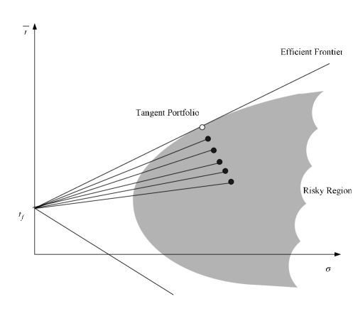
Figure 4: Admissible Region: Single-Period Case

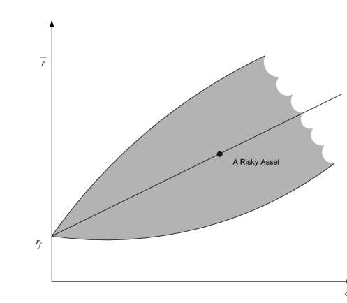
Figure 5: Combination of the Risk-Free Asset and a Risky One: Continuous-Time Case

Now, in the continuous-time case, let us also start with two assets, a risk-free asset represented by the portfolio $\pi_{f}(\cdot)\equiv 0$, and a risky asset represented by $\pi(\cdot)\neq\pi_{f}(\cdot)$. We use these two assets to form new portfolios of the form $\pi_{\alpha}(t)=[1-\alpha(t)]\pi_{f}(t)+\alpha(t)\pi(t)\equiv\alpha(t)\pi(t)$, where $\alpha(\cdot)$ is any progressively measurable process so long as $\pi_{\alpha}(\cdot)$ is admissible. Let $x(\cdot)$ be the wealth process corresponding to $\pi(\cdot)$. If $\alpha(t)\equiv\alpha\in\Re$; that is, the corresponding $\pi_{\alpha}(\cdot)$ is a buy and hold combination of the two, then it is immediate from the linearity of the wealth equation (2.4) that $\alpha x(\cdot)$ is the wealth process corresponding to $\pi_{\alpha}(t)$ whose terminal $(\sigma,\bar{r})$-value lies on the straight line connecting those of the two original assets. However, in general $\alpha(\cdot)$ can be any appropriate stochastic process (in other words, the new portfolio $\pi_{\alpha}(\cdot)$ is in general a dynamic combination of the two assets); so $\alpha(\cdot)x(\cdot)$ is no longer necessarily the wealth process under $\pi_{\alpha}(\cdot)$ or it may not lie on the straight line connecting the two original assets. As a consequence, all the new portfolios (with all the possible processes $\alpha(\cdot)$) forming from the original two assets generate a much larger region as indicated in Figure 5.

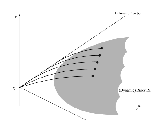
Figure 6: Admissible Region: Continuous-Time Case

To discuss on the shape of the admissible region in the continuous-time case (to be precise we are only interested in the upper left boundary of the admissible region), we first construct the dynamic risky region defined by the risky assets only, which is the shaded region in Figure 6. Next, for each portfolio in this region we make combinations with the risk-free asset. As discussed above these new portfolios form a solid two-dimensional region with its upper left boundary being a curved line in general (which could be a straightline in some special cases – such as the Black–Scholes case). There is such a curved line corresponding to every asset in the risky region. The envelope of these lines forms the upper left boundary of the entire admissible region (containing both the risk-free and risky assets), which is the efficient frontier we are seeking. It is these curved lines that push the efficient frontier away from the risky region; and hence the surprising phenomenon stipulated in Theorem 1.

Last but not least, the fact that in continuous time the mean–variance efficient frontier is still a straight line, derived in Bajeux-Besnainous and Portait (1998) and Zhou and Li (2000), is no longer a mere routine extension of its single-period counterpart, and should not be taken lightly. In fact, the efficient frontier is the envelope of infinitely many curved lines, which turns out to be a straight line. This is quite an unusual coincidence, indeed.

6. CONCLUDING REMARKS

This paper disclosed some rather unexpected phenomena associated with a continuous-time mean–variance market, suggesting that continuous-time financial models have more complex, sometimes strikingly different, structures and properties than its single-period counterpart. One should appreciate that continuous-time is probably a closer representation of the real-world investment today than its discrete-time counterpart, not to mention its analytical tractability which enables us to elicit important economic insights from results that are often explicit. On the other hand, in the realm of continuous-time asset allocation and asset pricing the literature has been dominated by the expected utility maximization (EUM) models. However, “few if any agents know their utility functions; nor do the functions which financial engineers and financial economists find analytically convenient necessarily represent a particular agent’s attitude towards risk and return” [Markowitz (2004)]. It is fair to say mean–variance (including the related Sharpe ratio) remains nowadays one of the most commonly used measures to assess the performance of fund managers. Theoretically, while mean–variance has some inherent drawbacks such as the sensitivity of the final solutions on the investment opportunity set, and the inconsistency with the dynamic programming principle in the continuous-time setting, recent studies have revealed some redeeming quality of continuous-time mean–variance efficient policies. For example, it is shown in Li and Zhou (2006) that, under the same setting as in this paper, a mean–variance efficient portfolio realizes the (discounted) targeted return on or before the terminal date with a probability greater than $0.8072$. This number is universal irrespective of the opportunity set, the targeted return, and the investment horizon. This, together with the new findings in this paper, suggests that it is necessary and important to revisit mean–variance models, in terms of both asset allocation and asset pricing, for dynamic markets.

In this paper there are several assumptions on the underlying model, such as free of transaction cost, market completeness, and deterministic investment opportunity set. Mean–variance models with proportional transaction costs have been recently studied by Dai, Xu and Zhou (2008). It would therefore be interesting to extend the results of this paper to the case with transaction costs. On the other hand, we believe our results can be extended to the incomplete market case, noting the results on mean–variance model in an incomplete market by Lim (2004). The case with stochastic investment opportunity, however, is still open, as Theorems 1 – 1 may no longer hold true.

Appendix: Proofs

Proof of Theorem 1: The assertion about the feasibility of the problem is an immediate consequence of Lim and Zhou (2002), Corollary 5.1. The efficient feedback strategies (3.2) and the expression (3.4) are derived in Zhou and Li (2000), eq. (5.12) and Thm. 6.1. Finally, that $\gamma>0$ is seen from the facts that $x_{0}>0$, $z\geq x_{0}e^{\int_{0}^{T}r(t)dt}$ and $|\theta(t)|>0$ (due to $B(t)\neq 0$) $\mbox{{\rm a.e.} }t\in[0,T]$. Q.E.D.

Proof of Theorem 1: To prove this theorem we need the following technical lemma.

LEMMA 6.1: For any $b>0$

(6.1) $$(e^{bx}-1)(e^{\frac{b}{x}}-1)\geq(e^{b}-1)^{2}\;\;\;\forall x>0.$$

Proof: The case when $x=1$ is trivial. Hence due to the symmetry we need only to show (6.1) for any $0<x<1$.

Let $f(x)=(e^{bx}-1)(e^{\frac{b}{x}}-1)$, $0<x\leq 1$. Then

$$f^{\prime}(x)=be^{\frac{b}{x}+bx}\left(1-\frac{1}{x^{2}}+\frac{1}{x^{2}}e^{-bx}-e^{{\color[rgb]{1,0,0}-}\frac{b}{x}}\right).$$

Denote $g(x)=1-\frac{1}{x^{2}}+\frac{1}{x^{2}}e^{-bx}-e^{-\frac{b}{x}}$, $0<x\leq 1$. We have

$$\begin{array}[]{llll}g^{\prime}(x)&=&\frac{1}{x^{3}}(2-2e^{-bx}-bxe^{-bx}-bxe^{-\frac{b}{x}})&\\ &>&\frac{2}{x^{3}}\left[1-(1+bx)e^{-bx}\right]&\\ &>&0,&\forall 0<x<1.\end{array}$$

So $g(x)<g(1)=0$ $\forall 0<x<1$, or $f^{\prime}(x)<0$ $\forall 0<x<1$. This leads to $f(x)\geq f(1)=(e^{b}-1)^{2}$. Q.E.D.

We now prove Theorem 1, which is to show that

(6.2) $$\frac{E[R^{*}(T)]-R_{f}(T)}{\sigma_{R^{*}(T)}}>\frac{E[R(T)]-R_{f}(T)}{\sigma_{R(T)}},$$

where $R^{*}(T)$ is the rate of return of any efficient portfolio, $R_{f}(T)$ is the risk free rate of return, and $R(T)$ is the rate of return of the risky asset, over $[0,T]$. Note $E[R(T)]=e^{\mu T}-1$, $\sigma_{R(T)}^{2}=e^{(2\mu+\sigma^{2})T}-e^{2\mu T}$, and $R_{f}(T)=e^{rT}-1$. So according to (3.6), (6.2) is equivalent to

(6.3) $$e^{(\frac{\mu-r}{\sigma})^{2}T}-1>\frac{(e^{\mu T}-e^{rT})^{2}}{e^{(2\mu+\sigma^{2})T}-e^{2\mu T}}.$$

Now,

$$e^{(\frac{\mu-r}{\sigma})^{2}T}-1-\frac{(e^{\mu T}-e^{rT})^{2}}{e^{(2\mu+\sigma^{2})T}-e^{2\mu T}}=\frac{e^{2\mu T}(e^{\sigma^{2}T}-1)\left(e^{((\mu-r)^{2}/\sigma^{2})T}-1\right)-e^{2rT}(e^{(\mu-r)T}-1)^{2}}{e^{(2\mu+\sigma^{2})T}-e^{2\mu T}}.$$

Considering the numerator of the above and noting $\mu>r$, we have

$$\begin{array}[]{lll}&e^{2\mu T}(e^{\sigma^{2}T}-1)(e^{((\mu-r)^{2}/\sigma^{2})T}-1)-e^{2rT}(e^{(\mu-r)T}-1)^{2}\\ >&e^{2\mu T}[(e^{\sigma^{2}T}-1)(e^{((\mu-r)^{2}/\sigma^{2})T}-1)-(e^{(\mu-r)T}-1)^{2}]&\\ >&(e^{\sigma^{2}T}-1)(e^{((\mu-r)^{2}/\sigma^{2})T}-1)-(e^{(\mu-r)T}-1)^{2}.&\end{array}$$

Letting $(\mu-r)T=b$ and $\sigma^{2}=(\mu-r)x$ where $x>0$, we have

$$\begin{array}[]{lll}&(e^{\sigma^{2}T}-1)(e^{((\mu-r)^{2}/\sigma^{2})T}-1)-(e^{(\mu-r)T}-1)^{2}&\\ =&(e^{bx}-1)(e^{b/x}-1)-(e^{b}-1)^{2}\\ \geq&0&\end{array}$$

by virtue of Lemma 1. The proof is complete. Q.E.D.

Proof of Theorem 1: Set $y(t):=x^{*}(t)-\gamma e^{-\int_{t}^{T}r(s)ds}$. Using the wealth equation (2.4) that $x^{*}(\cdot)$ satisfies and applying (3.2), we deduce

$$\left\{\begin{array}[]{l}dy(t)=[r(t)-|\theta(t)|^{2}]y(t)dt-\theta(t)y(t)dW(t),\\ y(0)=\frac{x_{0}-ze^{-\int_{0}^{T}r(t)dt}}{1-e^{-\int_{0}^{T}|\theta(t)|^{2}dt}}\leq 0.\end{array}\right.$$

The above equation has a unique solution

$$y(t)=y(0)\exp\left\{\int_{0}^{t}[r(s)-\frac{3}{2}|\theta(s)|^{2}]ds-\int_{0}^{t}\theta(s)dW(s)\right\}\leq 0,$$

and the inequality is strict if and only if $y(0)<0$, or $z>x_{0}e^{\int_{0}^{T}r(t)dt}$. Q.E.D.

Proof of Theorem 1: Since $x^{*}(t)\neq\gamma e^{-\int_{t}^{T}r(s)ds}$, the result follows directly from Theorem 1 and (3.2). Q.E.D.

Proof of Theorem 1: If $z=x_{0}e^{\int_{0}^{T}r(t)dt}$, then the theorem holds trivially. So we assume that $z>x_{0}e^{\int_{0}^{T}r(t)dt}$. According to Theorem 1, $\pi^{*}(\cdot)$ can be written as

(6.4) $$\pi^{*}(t)\equiv(\pi_{1}^{*}(t),\cdots,\pi_{m}^{*}(t))^{\prime}=-[\sigma(t)\sigma(t)^{\prime}]^{-1}B(t)[x^{*}(t)-\gamma e^{-\int_{t}^{T}r(s)ds}],$$

for some $\gamma>0$. If (4.5) is not true, then there is $\bar{t}\in(0,T]$ such that $P\{\pi_{0}^{*}(\bar{t})=0\}=1$, or

(6.5) $$P\{x^{*}(\bar{t})=\sum_{i=1}^{m}\pi_{i}^{*}(\bar{t})\}=1.$$

Summing all the components of $\pi^{*}(t)$ in (6.4) at $t=\bar{t}$, we have

(6.6) $$x^{*}(\bar{t})=\sum_{i=1}^{m}\pi_{i}^{*}(\bar{t})=-\eta(\bar{t})[x^{*}(\bar{t})-\gamma e^{-\int_{\bar{t}}^{T}r(s)ds}],$$

where $\eta(t):={\bf e}^{\prime}[\sigma(t)\sigma(t)^{\prime}]^{-1}B(t)$ with ${\bf e}=(1,1,\cdots,1)^{\prime}$. Note that $\eta(t)\neq-1\;\forall t\in[0,T)$, for otherwise (6.6) would yield $\gamma=0$, contradicting (3.3). Hence, it follows from (6.6) that

(6.7) $$x^{*}(\bar{t})=\frac{\gamma\eta(\bar{t})e^{-\int_{\bar{t}}^{T}r(s)ds}}{1+\eta(\bar{t})}.$$

In other words, the wealth at time $\bar{t}$ is a deterministic quantity.

However, the wealth equation (2.4) that $x^{*}(\cdot)$ satisfies up to the time $\bar{t}$ can be rewritten as

(6.8) $$\left\{\begin{array}[]{l}dx^{*}(t)=[r(t)x^{*}(t)+\theta(t)(\sigma(t)^{\prime}\pi^{*}(t))]dt+(\sigma(t)^{\prime}\pi^{*}(t))^{\prime}dW(t),\;\;t\in[0,\bar{t}),\\ x^{*}(\bar{t})=\frac{\gamma\eta(\bar{t})e^{-\int_{\bar{t}}^{T}r(s)ds}}{1+\eta(\bar{t})}.\end{array}\right.$$

The above is a linear backward stochastic differential equation (BSDE) with deterministic linear coefficients as well as a deterministic terminal condition. Hence by the uniqueness of its solution we must have $\sigma(t)^{\prime}\pi^{*}(t)=0\;\;\mbox{{\rm a.s.}},\;\mbox{{\rm a.e.}}\;t\in[0,\bar{t}]$. Appealing to (2.3), we conclude that $\pi^{*}(t)={0}$, a.s., $\mbox{{\rm a.e.}}\;t\in[0,\bar{t}].$ This in turn implies $B(t)=0$ $\forall t\in[0,\bar{t}]$, in view of (6.4), Theorem 1, and the fact that $B(t)$ is continuous in $t$. So $\eta(t)=0$, $\forall t\in[0,\bar{t}]$, and hence $x^{*}(\bar{t})=0$. Again by the uniqueness of solution to BSDE (6.8), $x_{0}=0$, which is a contradiction. Q.E.D.

REFERENCES

Bajeux-Besnainous, L., and R. Portait (1998): “Dynamic Asset Allocation in a Mean—Variance Framework,” Management Sciences, 44, 79–95.

Dai, M., Z. Xu, and X.Y. Zhou (2008): “Continuous-Time Mean–Variance Portfolio Selection with Proportional Transaction Costs,” Working paper, University of Oxford.

KARATZAS, I., AND S.E. SHREVE (1999): Methods of Mathematical Finance. New York: Springer-Verlag.

Li, D., and W.L. Ng (2000): “Optimal Dynamic Portfolio Selection: Multi-period Mean-Variance Formulation,” Mathematical Finance, 10, 387–406.

Lim, A.E.B. (2004): “Quadratic Hedging and Mean–Variance Portfolio Selection with Random Parameters in an Incomplete Market,” Mathematics of Operations Research, 29, 132–161.

LIM, A.E.B., AND X.Y. ZHOU (2002): “Mean-Variance Portfolio Selection with Random Parameters in a Complete Market,” Mathematics of Operations Research, 27, 101–120.

Li, X. and X.Y. Zhou (2006): “Continuous-Time Mean–Variance Efficiency: The 80% Rule,” Annals of Applied Probability, 16, 1751–1763.

LINTNER, J. (1965): “The Valuation of Risk Assets and The Selection of Risky Investments in Stock Portfolios and Capital Budgets,” Review of Economics and Statistics, 47, 13–37.

Luenberger D.G. (1998): Investment Science, Oxford University Press, New York.

MARKOWITZ, H. (1952): “Portfolio Selection,” Journal of Finance, 7, 77–91.

——– (1987): Mean–Variance Analysis in Portfolio Choice and Capital Markets. New Hope, Pennsylvania: Frank J. Fabozzi Associates.

MARKOWITZ, H., AND X.Y. ZHOU (2004): Private communication.

MERTON, R.C. (1972): “An Analytic Derivation of the Efficient frontier,” Journal of Financial and Quantitative Analysis, 7, 1851–1872.

MOSSIN, J. (1966): “Equilibrium in a Capital Asset Market,” Econometrica, 34, 768–783.

Richardson, H.R. (1989): “A Minimum Variance Result in Continuous Trading Portfolio Optimization,” Management Sciences, 25, 1045–1055.

SHARPE, W.F. (1964): “Capital Asset Prices: A Theory of Market Equilibrium under Conditions of Risk,” Journal of Finance, 19, 425–442.

TOBIN, J. (1958): “Liquidity Preference as Behavior Towards Risk,” The Review of Economic Studies, 25, 65–86.

Zhou, X.Y., and D. Li (2000): “Continuous-Time Mean-Variance Portfolio Selection: A Stochastic LQ Framework,” Applied Mathematics and Optimization, 42, 19–33.