Edge-locking and quantum control in highly polarized spin chains

Abstract

For an open-boundary spin chain with anisotropic Heisenberg (XXZ) interactions, we present states in which a connected block near the edge is polarized oppositely to the rest of the chain. We show that such blocks can be ‘locked’ to the edge of the spin chain, and that there is a hierarchy of edge-locking effects at various orders of the anisotropy. The phenomenon enables dramatic control of quantum state transmission: the locked block can be freed by flipping a single spin or a few spins.

Introduction — Quantum state transfer, and more generally the control of quantum states, has in recent years entered the realm of experimental possibilities due to rapid advances in nanostructure and cold-atom technologies, and as a result has been the focus of intense theory interest Bose_PRL03 ; Bose_ContemPhys07 ; ChristandlDattaEkertLandahl_PRL04 ; RomitoFazioBruder_PRB05 ; DeChiaraRossiniMontangeroFazio_PRA05 ; RossiniGiovannettiMontangero_NJP08 ; Romero-IsartEckertSanpera_PRA07 ; KarbachStolze_PRA05 ; LyakhovBruder_NJP05 . More generally, explicit temporal evolution of many-body quantum states far from equilibrium are no longer of academic interest only, as was the case in the traditional bulk solid-state context.

In this work, we present and analyze a phenomenon associated with the high-energy spectrum of open-boundary spin chains, namely, the locking of spin states by the edge. We also show how this ‘edge-locking’ effect can be exploited to exert control over state propagation and spin transfer processes in spin chains.

We will consider spin-$\frac{1}{2}$ chains governed by an anisotropic Heisenberg interaction, i.e., $XXZ$ chains. We consider highly polarized states, and show that a block of spins anti-aligned to this background can have stable positions if placed appropriately at or near the edge. We reveal the sense in which these configurations are close to being stationary states of the Hamiltonian. The presence of such stable arrangements, and the possibility to convert to non-stable formations via operations on a few spins, open up simple but powerful possibilities for controlling spin state propagation.

The $XXZ$ chain is a basic model of condensed matter physics, and has long been the subject of sustained theoretical activity. The open chain has received far less detailed attention than the periodic case, and even less material is available for physics far from the ground state. A new localization phenomenon associated with the $XXZ$ chain is thus obviously of fundamental interest. In addition, the $XXZ$ model has recently been shown to describe Josephson junction arrays of the flux qubit type LyakhovBruder_NJP05 , and may also be realizable in optical lattices DuanDemlerLukin_PRL03 . The mechanisms for quantum control uncovered by our results should be possible to implement in one of these setups in the foreseeable future.

Hamiltonian — The open antiferromagnetic $XXZ$ chain with $L$ sites is described by the Hamiltonian

$$H_{XXZ}~{}=~{}J_{x}\sum_{j=1}^{L-1}\left[S_{j}^{x}S_{j+1}^{x}+S_{j}^{y}S_{j+1}^{y}~{}+~{}{\Delta}S_{j}^{z}S_{j+1}^{z}\right]\;.$$

The $S^{z}S^{z}$ term acts as an ‘interaction’ penalizing alignment of neighboring spins. The in-plane terms $(S_{j}^{x}S_{j+1}^{x}+S_{j}^{y}S_{j+1}^{y})=\tfrac{1}{2}(S_{j}^{+}S_{j+1}^{-}+S_{j}^{-}S_{j+1}^{+})$ provide ‘hopping’ processes relevant for quantum state transfer. Since $H_{XXZ}$ preserves total $S^{z}$, the dynamics is always confined to sectors of fixed numbers $N_{\uparrow}$ of up-spins. We will mostly consider the large $\Delta$ regime, where the localization phenomena to be described are most robust. Energy and time are measured in $J_{z}=J_{x}\Delta$ and $J_{z}^{-1}=(J_{x}\Delta)^{-1}$ units unless stated otherwise.

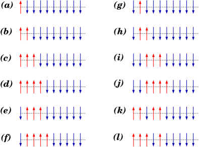
Figure 1: (Color online.) A few $\uparrow$ spins at the left edge of an almost polarized spin chain. The leftmost 10 spins are shown; the remaining spins to the right are all $\downarrow$’s. Configurations a–f are edge-locked, while g–l are not.

Edge-locked states — In Fig. 1 we show some example configurations, i.e., positions of spin-up blocks near the edge, in a background of down spins. In the configurations shown on the left, the $\uparrow$ blocks are locked by the edge at large $\Delta$, while the blocks in the right-column configurations are not edge-locked. In dynamic terms, this means that the configurations on the left column are stable, while those shown on the right decay away. Of course, ‘stability’ should be understood in terms of timescales relevant to the edge-locking physics, and are not absolute.

The simplest and most robust edge states are those in which the block starts at the very edge site, such as configurations a through d in Fig. 1. Even a single $\uparrow$ spin placed in this way is localized at the edge. For $N_{\uparrow}$ up-spins placed this way, we call these configurations $\left|{L_{N_{\uparrow},(1)}}\right.\rangle$ or $\left|{R_{N_{\uparrow},(1)}}\right.\rangle$, depending on whether the block is at the left edge or right edge of the chain. Figs. 1a through 1d are thus $\left|{L_{1,(1)}}\right.\rangle$ through $\left|{L_{4,(1)}}\right.\rangle$. The subscript ‘(1)’ indicates that the $\uparrow$-blocks start at the very edge site.

The second class of edge states are those where the block starts at the $j=2$ site (or ends at $j=L-1$). We call these $\left|{L_{N_{\uparrow},(2)}}\right.\rangle$ or $\left|{R_{N_{\uparrow},(2)}}\right.\rangle$. For such states to be edge-locked, one needs blocks of three or more $\uparrow$’s, i.e., $N_{\uparrow}\geq 3$. This is indicated in Fig. 1 by showing $\left|{L_{1,(2)}}\right.\rangle$, $\left|{L_{2,(2)}}\right.\rangle$ on the right column (not edge-locked) as g, h, and $\left|{L_{3,(2)}}\right.\rangle$, $\left|{L_{4,(2)}}\right.\rangle$ on the left column (edge-locked) as e, f. Similarly, blocks starting at $j=3$ (or ending at $j=L-2$) are stable only for $N_{\uparrow}\geq 5$. Generalizing, state $\left|{L_{N_{\uparrow},(k)}}\right.\rangle$ having a block starting at site $k$ will be stable via edge-locking only if $N_{\uparrow}{\geq}(2k-1)$.

The edge-locking effects are due to spectral separation of the stable states from other states, which prevents hybridizations that might enable propagation of the oppositely-polarized blocks. The spectral separation can be understood using perturbative arguments at small $\Delta^{-1}$. In the hierarchy described above, the first class of edge-locking (blocks starting at the edge site) is a zeroth-order effect, while edge-locking at the second level (blocks starting at next-to-edge site) is an $\mathcal{O}(\Delta^{-2})$ effect. Generally, the level-$k$ edge-locking of this hierarchy is an $\mathcal{O}(\Delta^{-2(k-1)})$ effect.

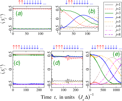
Figure 2: (Color online.) Dynamics of 18-site open $XXZ$ chain ($\Delta=4$), initiated with $N_{\uparrow}=2$ or $N_{\uparrow}=3$ oppositely-polarized spins near the left edge. Initial configurations are shown on top of each panel. In the edge-locked cases, local spin values $\langle{S_{j}^{z}}\rangle$ do not vary much from their initial values.

Temporal dynamics — Fig. 2 demonstrates the edge-locking phenomenon through explicit time evolution of several configurations. The top row shows the evolution of $N_{\uparrow}=2$ states $\left|{L_{2,(1)}}\right.\rangle$ and $\left|{L_{2,(2)}}\right.\rangle$. The first is an edge-locked state and shows very little evolution, while the second is not locked, and thus the $\uparrow\uparrow$ block propagates to the right.

The bottom row shows $N_{\uparrow}=3$ states. Now there are two states where the $\uparrow\uparrow\uparrow$ block is locked by the left edge. We have chosen a moderate value of $\Delta$ so that the $\mathcal{O}(\Delta^{-2})$ locked state $\left|{L_{3,(2)}}\right.\rangle$ can be clearly seen to have weaker locking than the $\mathcal{O}(\Delta^{0})$ locked state $\left|{L_{3,(1)}}\right.\rangle$. (Fig. 2d has more dynamics and larger oscillations than 2c.) Obviously, the higher-order locking can be made more robust by using a larger $\Delta$.

The numerical results of Fig. 2 are for 18-site open chains, but a longer chain would display identical time evolutions at the time scales shown. The size plays a role only when the propagating block meets the other edge and gets reflected. It is clear that the unlocked blocks in Fig. 2 (b,e) are still propagating to the right at the timescales shown.

Spectral explanation — We now turn to the spectral separation that causes edge-locking by suppressing hybridization with non-locked states. Fig. 3 shows the energy spectrum for $L=13$ sites, in the $N_{\uparrow}=3$ sector. At large $\Delta$, the spectrum separates into well-separated ‘bands’. In the periodic chain, the bands correspond to cases where the three $\uparrow$ spins are next to each other (top band), or two are next to each other (middle band), or no two $\uparrow$ spins neighbor each other (bottom band). In general, with $N_{\uparrow}$ ($<L/2$) up spins in a periodic large-$\Delta$ chain, the spectrum is separated into $p(N_{\uparrow})$ bands, where $p(n)$ is the number of integer partitions of $n$. The topmost band is maximally ferromagnetic, and has the minimal number (two) of favorable $\uparrow$-$\downarrow$ bonds and ($L-2$) non-favorable ($\uparrow$-$\uparrow$ or $\downarrow$-$\downarrow$) bonds.

Fig. 3b shows the effect of open boundaries. The spectrum described above for the periodic chain now acquires an explosion of additional features. The periodic-chain bands get split, because the edge allows additional possibilities for numbers of favorable and unfavorable bonds. In addition, several of these new bands have additional sub-structures, as shown in insets. While these structures are all interesting, in this work we will only be concerned with the top two bands of the open chain, which both emerge from the topmost band of the periodic chain, and hence are related to periodic-chain configurations with all $\uparrow$ spins in a connected block.

The top-most band has only two states, and these are the most obvious edge-locked states. For three up spins at $\Delta^{-1}=0$, this is a degenerate two-dimensional manifold spanned by $\left|{L_{3,(1)}}\right.\rangle=\left|{\uparrow\uparrow\uparrow\downarrow\downarrow\downarrow\downarrow\downarrow...}\right.\rangle$ and $\left|{R_{3,(1)}}\right.\rangle=\left|{...\downarrow\downarrow\downarrow\downarrow\downarrow\uparrow\uparrow\uparrow}\right.\rangle$. At finite $\Delta^{-1}$, other configurations contribute to the two states, but for small enough $\Delta^{-1}$ the eigenstates are dominated by $\left|{L_{3,(1)}}\right.\rangle\pm\left|{R_{3,(1)}}\right.\rangle$. Similarly, for other values of $N_{\uparrow}$, the topmost eigenstates are dominated by $\left|{L_{N_{\uparrow},(1)}}\right.\rangle\pm\left|{R_{N_{\uparrow},(1)}}\right.\rangle$ at large $\Delta$. These two states appear at the very top because $\left|{L_{N_{\uparrow},(1)}}\right.\rangle$ and $\left|{R_{N_{\uparrow},(1)}}\right.\rangle$ are the only configurations having a single favorable anti-aligned bond and thus a maximum number ($L-2$) of unfavorable bonds. In contrast, in the periodic case any configuration has at least two favorable bonds.

The edge block in $\left|{L_{N_{\uparrow},(1)}}\right.\rangle$ is strongly locked because this state is hybridized mainly with $\left|{R_{N_{\uparrow},(1)}}\right.\rangle$. From $\left|{L_{N_{\uparrow},(1)}}\right.\rangle$, it is energetically possible to tunnel into the $\left|{R_{N_{\uparrow},(1)}}\right.\rangle$ state, but such a process is exponentially suppressed at large chain lengths. Thus $\left|{L_{N_{\uparrow},(1)}}\right.\rangle$ can be regarded as ‘stationary’ for practical purposes, as Fig. 2(a,c) demonstrates dynamically.

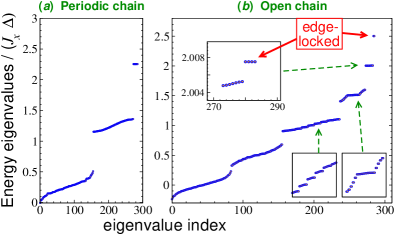
Figure 3: (Color online.) Energy spectra: $L=13$, $N_{\uparrow}=3$, $\Delta=10$. Compared to the periodic chain, the open chain spectrum has extra features, some of which are highlighted in insets. With $N_{\uparrow}=3$, there are two classes of edge-locked states, the two states of the top band (main plot) and two of the four states separating out from the next band (upper inset).

The other edge-locking effects are weaker and can be seen by zooming into the second band from the top, which consists of configurations with two favorable bonds (Fig. 3b upper inset). Four states separate out from the rest of this band, with $\mathcal{O}(\Delta^{-2})$ splitting. These four states are linear combinations of $\left|{L_{3,(2)}}\right.\rangle$, $\left|{R_{3,(2)}}\right.\rangle$, and

$$\left|{\uparrow\uparrow\downarrow\downarrow\downarrow.....\downarrow\downarrow\downarrow\uparrow}\right.\rangle\quad{\rm and}\quad\left|{\uparrow\downarrow\downarrow\downarrow.....\downarrow\downarrow\downarrow\uparrow\uparrow}\right.\rangle\;.$$

The rest of the band is dominated by linear combinations of the remaining configurations containing the $\uparrow$ spins in connected blocks farther from the edge.

Due to the spectral separation, the four states are not hybridized with the remaining block configurations. This locks the $\left|{L_{3,(2)}}\right.\rangle$ and $\left|{R_{3,(2)}}\right.\rangle$ configurations to their respective edges, because from any of these states, tunneling to the other three of the sub-manifold is a very high-order process in $J_{x}$.

Hierarchy in spectrum — For $N_{\uparrow}=3$, only the first two classes of edge-locked states are present, as indicated by the two solid arrows in Fig. 3b. An additional level of the hierarchy becomes available with each increase of $N_{\uparrow}$ by two. The associated spectral separations can be seen by successively zooming in, within the next-to-top band. Fig. 4 (left three panels) shows this for $N_{\uparrow}=5$, where three edge-locked configurations appear. Fig. 4 (right) displays the associated gaps scaling as $\delta_{k}\sim\Delta^{2k-1}$.

Physical reason for spectral separation — The spectral separations leading to edge-locking can be understood through degenerate perturbation theory. We give a brief explanation for the second level, namely the separation of states $\left|{L_{N_{\uparrow},(2)}}\right.\rangle$ and $\left|{R_{N_{\uparrow},(2)}}\right.\rangle$ from the states $\left|{L_{N_{\uparrow},(k)}}\right.\rangle$ with $2<k<(L-1)$.

At $\Delta^{-1}=0$, the configurations with two favorable bonds are all degenerate. At small finite $\Delta^{-1}$ these spread out to form the next-to-top band. The hybridization of these levels happens at order $\Delta^{-N_{\uparrow}}$, because $N_{\uparrow}$ ‘hoppings’ are required to connect configurations $\left|{L_{N_{\uparrow},(k)}}\right.\rangle$ and $\left|{L_{N_{\uparrow},(k+1)}}\right.\rangle$.

On the other hand, since each $\left|{L_{N_{\uparrow},(k)}}\right.\rangle$ is connected to itself by two hoppings, the states acquire energy shifts at order $\Delta^{-2}$. Considering the energies of the intermediate states in this process, one can see that the states $\left|{L_{N_{\uparrow},(2)}}\right.\rangle$ and $\left|{R_{N_{\uparrow},(2)}}\right.\rangle$ have a different energy shift compared to the rest, due to the edge. For $N_{\uparrow}>2$ this $\mathcal{O}(\Delta^{-2})$ effect is stronger than the $\mathcal{O}(\Delta^{-N_{\uparrow}})$ hybridization, so that these states separate out without hybridizing with the rest, and are thus edge-locked.

The argument can be extended to higher stages of the hierarchy. Blocks starting at site $k$ have a $\mathcal{O}(\Delta^{-2(k-1)})$ shift distinct from the shift of the farther blocks, and hence will be separated from the band if $2(k-1)<N_{\uparrow}$, allowing further edge-locked configurations.

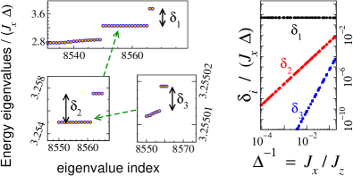
Figure 4: (Color online.) Left: hierarchy of sub-band splittings seen by zooming in successively. Here $N_{\uparrow}=5$ ($L=18$, $\Delta=10$), so the first three levels of the hierarchy are present. Right: Energy splittings scale as $\delta_{1}\sim\Delta^{0}$, $\delta_{2}\sim\Delta^{-2}$, $\delta_{3}\sim\Delta^{-4}$.

State transfer protocols — The edge-locking phenomenon provides many opportunities for controlling the evolution and transport of spin states, provided that the experimental realization of the $XXZ$ chain allows single-site (or few-site) addressing. We point out a few of the most obvious quantum control protocols.

If single-site spin flipping probes ($\pi$ pulse) can be implemented, this can be used to ‘release’ a locked block. For example, by flipping the first spin of the locked block in $\left|{L_{3,(1)}}\right.\rangle$, one gets the state $\left|{L_{2,(2)}}\right.\rangle$, in which the two-site block is not locked (Fig. 2b), and so starts propagating. Similarly, starting with a 5- or 6-site oppositely-polarized block at the edge, applying a $\pi$ pulse on the first two sites initiates the transmission of a signal consisting of a block of spins anti-aligned to the background. Once the signal reaches the other edge of the open chain, the block could also be locked to the other edge by $\pi$-pulsing one or two spins at the other edge at the appropriate moment.

More complex dynamics can be launched by applying a $\pi$ pulse to a site internal to the locked block, for example, by flipping the second site of the locked $\left|{L_{4,(1)}}\right.\rangle$ configuration. The resulting $\uparrow\downarrow\uparrow\uparrow\downarrow\downarrow\downarrow\downarrow....$ has the following dynamics: the $\uparrow$ at site 3 moves to site 2 so that a two-site $\uparrow\uparrow$ block then stays locked to the edge, while a third $\uparrow$ propagates to the right. While a complete explanation involves the lower energy bands, which are beyond the scope of this paper, the tendency to lock blocks at the edge is clearly seen here too.

The hierarchy structure can be also used to design more subtle control protocols, for example, a $\pi$ pulse can be used to go from a strongly locked state to a weakly locked state; the difference is especially acute at moderate $\Delta\gtrsim 1$. For example, starting with $\left|{L_{4,(1)}}\right.\rangle$ and flipping the first spin performs such an operation.

Spinless fermion model — The $XXZ$ chain model is generally considered to be equivalent to the spinless fermion model with nearest-neighbor couplings. However, if the interaction is of $Vn_{i}n_{i+1}$ form ($n_{i}$ are site occupancies), the spectral structure associated with open-chain edge-localization is quite different from the $XXZ$ chain, as can be seen by comparing present results with Ref. PintoHaqueFlach_PRA09 . The physics becomes identical if one uses the $V(n_{i}-\tfrac{1}{2})(n_{i+1}-\tfrac{1}{2})$ form, which involves interactions between unoccupied sites.

Experimental realizations — The most obvious realizations are bulk materials with chain structures. There are several compounds whose spin physics are reasonably well-described by $\Delta>1$ $XXZ$ Hamiltonians, such as CsCoCl₃ with $\Delta\sim 7$ YoshizawaHirakawaSatijaShirane_PRB81 ; GoffTennantNagler_PRB95 , and BaCo₂V₂O₈ with $\Delta\sim 2$ KimuraOkunishi-etal_PRL07 . Unfortunately, single-site addressing is generally not feasible, and nonequilibrium states generally relax rapidly to the ground state in bulk materials. Nevertheless, it may still be possible to probe the physics presented in this paper. With the spins polarized completely by a magnetic field above the saturation threshold, a localized excitation (through neutrons or laser pulse) could depolarize a few sites, moving the system to a sector where edge states can be relevant. Applying an excitation near one end of the material, one can watch for response at the other end, which would indicate whether the excited block is locked or propagating.

A more promising route is through Josephson junction arrays, which in some arrangements (persistent-current qubits MooijOrlandoLevitov-etal_Science99 ; LevitovOrlandoMooij_arxiv01 ) are well-described by an $XXZ$ Hamiltonian LyakhovBruder_NJP05 . Such arrays could be prepared in non-equilibrium initial states and single-qubit addressing should be straightforward, and thus might be ideal for initial exploration of the physics described here.

Finally, there is the possibility of realizing $XXZ$ lattices in cold-atom setups DuanDemlerLukin_PRL03 , although this has additional complications of realizing a well-defined edge and accounting for harmonic traps.

Open issues — This work raises several issues demanding further investigation. One expects dynamical effects and additional localization phenomena associated with the sub-structures of the lower bands (Fig. 3), which are yet to be explored. Depending on the experimental realization(s) that become available, the effects of terms beyond the $XXZ$ Hamiltonian relevant for the particular realization need to be analyzed, and new control protocols can be designed for the site addressing methods that are possible. Finally, the $XXZ$ model being Bethe-ansatz solvable even with open boundary conditions Alcaraz-et-al_JPhysA87 , it remains an open problem to find out how the sub-band and edge-locking structures in the high-energy spectrum are reflected in the Bethe ansatz root structure.

The author thanks J.-S. Caux, S. Flach, A. M. Läuchli, and T. Vojta for helpful discussions.

References

- (1) S. Bose, Phys. Rev. Lett. 91, 207901 (2003).
- (2) S. Bose, Contemp. Phys. 48, 13 (2007).
- (3) M. Christandl, N. Datta, A. Ekert, and A. J. Landahl, Phys. Rev. Lett. 92, 187902 (2004).
- (4) A. Romito, R. Fazio, and C. Bruder, Phys. Rev. B 71, 100501 (2005).
- (5) G. De Chiara, D. Rossini, S. Montangero, and R. Fazio, Phys. Rev. A 72, 012323 (2005).
- (6) D. Rossini, V. Giovannetti and S. Montangero, New J. Phys. 10, 115009 (2008).
- (7) O. Romero-Isart, K. Eckert, and A. Sanpera, Phys. Rev. A 75, 050303(R) (2007).
- (8) P. Karbach and J. Stolze, Phys. Rev. A 72, 030301 (2005).
- (9) A. Lyakhov and C. Bruder, New J. Phys. 7, 181 (2005 ).
- (10) L.-M. Duan, E. Demler, and M. D. Lukin, Phys. Rev. Lett. 91, 090402 (2003).
- (11) R. A. Pinto, M. Haque, and S. Flach, Phys. Rev. A 79, 052118 (2009).
- (12) H. Yoshizawa, K. Hirakawa, S. K. Satija and G. Shirane, Phys. Rev. B 23, 2298 (1981).
- (13) J. P. Goff, D. A. Tennant, and S. E. Nagler, Phys. Rev. B 52, 15992 (1995).
- (14) S. Kimura et. al., Phys. Rev. Lett. 99, 087602 (2007).
- (15) J. E. Mooij et. al., Science 285, 1036 (1999).
- (16) L. S. Levitov et. al., cond-mat/0108266
- (17) F. C. Alcaraz et. al., J. Phys. A 20 6397 (1987).