Photometric Redshift Estimation Using Spectral Connectivity Analysis

Abstract

The development of fast and accurate methods of photometric redshift estimation is a vital step towards being able to fully utilize the data of next-generation surveys within precision cosmology. In this paper we apply a specific approach to spectral connectivity analysis (SCA; Lee & Wasserman 2009) called diffusion map. SCA is a class of non-linear techniques for transforming observed data (e.g., photometric colours for each galaxy, where the data lie on a complex subset of $p$-dimensional space) to a simpler, more natural coordinate system wherein we apply regression to make redshift predictions. In previous applications of SCA to other astronomical problems (Richards et al. 2009a, Richards et al. 2009b), we demonstrate its superiority vis-a-vis Principal Components Analysis (PCA), a standard linear technique for transforming data. As SCA relies upon eigen-decomposition, our training set size is limited to $\la$ 10⁴ galaxies; we use the Nyström extension to quickly estimate diffusion coordinates for objects not in the training set. We apply our method to 350,738 SDSS main sample galaxies, 29,816 SDSS luminous red galaxies, and 5,223 galaxies from DEEP2 with CFHTLS $ugriz$ photometry. For all three datasets, we achieve prediction accuracies on par with previous analyses, and find that use of the Nyström extension leads to a negligible loss of prediction accuracy relative to that achieved with the training sets. As in some previous analyses (e.g., Collister & Lahav 2004, Ball et al. 2008), we observe that our predictions are generally too high (low) in the low (high) redshift regimes. We demonstrate that this is a manifestation of attenuation bias, wherein measurement error (i.e., uncertainty in diffusion coordinates due to uncertainty in the measured fluxes/magnitudes) reduces the slope of the best-fit regression line. Mitigation of this bias is necessary if we are to use photometric redshift estimates produced by computationally efficient empirical methods in precision cosmology.

1 Introduction

The accurate estimation of redshifts from photometric data is a key component to fulfilling the promise of next-generation cosmological surveys. For instance, photometry to $R\sim$ 30 is expected for billions of galaxies from the Large Synoptic Survey Telescope (LSST; Ivezić et al. 2008) alone; compare this to, e.g., the $\sim$ 10⁵ spectra collected to a depth $R\sim$ 24 by the DEEP2 Galaxy Redshift Survey (Davis et al. 2003, Davis et al. 2007). It is clear that redshift-dependent analyses of galaxies that aim to undercover signatures of, e.g., weak lensing or baryon acoustic oscillations in imaging data will require the use of photometric redshifts.

Redshifts estimated via, e.g., $ugriz$ photometry will necessarily lack the precision of those that are spectroscopically derived due to noise, outliers, weak spectral features, and incomplete spectral energy distribution (SED) templates. For this reason, one major goal of photometric redshift estimation is to generate accurate ensembles of estimates, i.e., to have the mean redshift within a photometric redshift bin be an accurate estimator of true redshift (see, e.g., Albrecht et al. 2006, Ma, Hu, & Huterer 2006). Such ensembles are typically generated via one of two methods: either template fitting, wherein redshifted SED templates are generally compared to a given vector of magnitudes with the goal of minimizing the $\chi^{2}$ statistic or maximizing the likelihood (e.g., Fernández-Soto, Lanzetta, & Yahil 1999, Benítez 2000, Feldmann et al. 2006), or empirical methods, wherein one uses photometry from a small collection of objects with spectroscopically confirmed redshifts to train a model relating photometric colours to redshifts (e.g., Connolly et al. 1995, Vanzella et al. 2004, Collister & Lahav 2004, Budavári et al. 2005, Ball et al. 2007, Ball et al. 2008, Oyaizu et al. 2008). Some combine the two approaches (e.g., Ilbert et al. 2006, Ilbert et al. 2008), while others propose folding in information beyond photometric colours (e.g., Collister & Lahav 2004, Ball et al. 2004, Wray & Gunn 2008, Newman 2008).

In this paper we propose a new empirical method for photometric redshift estimation based on the diffusion map (Coifman & Lafon 2006, Lafon & Lee 2006), which is an approach to spectral connectivity analysis (SCA). SCA is a suite of established non-linear eigen-techniques that capture the underlying geometry of data by propagating local neighborhood information through a Markov process. SCA thus allows one to find a natural coordinate system for data such as photometric colours whose original parametrization is not amenable to available statistical techniques. In Richards et al. (2009a) and Richards et al. (2009b), we apply the diffusion map to two different astronomical problems. In Richards et al. (2009a), we develop a framework combining diffusion map and adaptive linear regression and apply it to SDSS spectroscopic data, demonstrating how it may be used to reduce the dimensionality of the data space and to predict, e.g., redshifts in a computationally efficient manner. We also demonstrate the superiority of the diffusion map to principal components analysis, a related, much more commonly used linear technique. In Richards et al. (2009b), we utilize the diffusion map and the K-means clustering algorithm to determine optimal bases of simple stellar population spectra that we use to estimate the star-formation histories of galaxies.

In §2, we review the basics of our diffusion map and regression framework, and introduce a new component: the application of the Nyström extension (see, e.g., Press et al. 1992), a computationally efficient and accurate technique for estimating diffusion coordinates for new objects given those of the training set. In §3, we apply our framework to Sloan Digital Sky Survey data, specifically main sample galaxies (MSGs) and luminous red galaxies (LRGs), and demonstrate that we achieve accuracy on par with that of more computationally intensive techniques. We also apply our framework to data from the DEEP2 Galaxy Redshift Survey that is matched to $ugriz$ photometry of the Canada-France-Hawaii Telescope Legacy Survey (CFHTLS; Gwyn 2008) and demonstate that it provides accurate estimation of redshifts to $z\approx 0.75$ given four colours alone. We demonstrate that the bivariate distributions of photometric and spectroscopic redshifts for SDSS and DEEP2 are affected by attenuation bias, the tendency of measurement error in the predictor to reduce the slope of linear models. Last, in §4, we summarize our results and discuss how we can extend our framework to the high redshift regime where spectroscopic coverage will be incomplete.

2 Algorithm

2.1 Diffusion map

In this section we review the basics of diffusion map construction, an approach to SCA. For more details, we refer the reader to Coifman & Lafon (2006), Lafon & Lee (2006), and Richards et al. (2009a). In Richards et al., we compare and contrast the use of diffusion maps with a more commonly utilized linear technique, principal components analysis, and demonstrate the superiority of diffusion maps in predicting spectroscopic redshifts of SDSS data from the galaxy spectra.

Here,“spectral connectivity analysis” refers to a class of methods which utilize a local distance measure to “connect” similar observations. The eigenmodes (i.e., “spectral decomposition”) of the rescaled matrix of similarities (see below for the definition of this matrix) can reveal a natural coordinate system for data that was absent in the original representation. For instance, imagine data in two dimensions that to the eye clearly exhibit spiral structure (e.g., fig. 1 of Richards et al. 2009a). For such data, the Euclidean distance between data points $\mn@boldsymbol{x}$ and $\mn@boldsymbol{y}$ would not be an optimal description of the ‘true’ distance between them along the spiral. Diffusion map is a leading example of an approach to SCA. In the diffusion map framework, the ‘true’ distance is estimated via a fictive diffusion process over the data, with one proceeding from $\mn@boldsymbol{x}$ to $\mn@boldsymbol{y}$ via a random walk along the spiral.

We construct diffusion maps as follows.

We define a similarity measure $s(\mn@boldsymbol{x},\mn@boldsymbol{y})$ that quantitatively relates two data points $\mn@boldsymbol{x}$ and $\mn@boldsymbol{y}$. In this work, a data ‘point’ is a vector of colours {$c_{1},\dots,c_{p}$} of length $p$ for a single galaxy, and the similarity measure that we apply is the Euclidean distance

$$s(\mn@boldsymbol{x},\mn@boldsymbol{y})~{}=~{}\sqrt{\sum_{i=1}^{p}\left(c_{\mn@boldsymbol{x},i}-c_{\mn@boldsymbol{y},i}\right)^{2}}\,.$$

A key feature of SCA is that the choice of $s(\mn@boldsymbol{x},\mn@boldsymbol{y})$ is not crucial, as it is often simple to determine whether or not two data points are ‘similar.’

We remove extreme outliers from our dataset, not because of their effect on diffusion map construction (a hallmark of the diffusion map is its robustness in the presence of outliers), but rather because they can bias the coefficients of the linear regression model (see §2.2) and because we find that individual predictions made for these objects are highly inaccurate. We compute the empirical distributions of Euclidean distances in colour space from each object to its $n^{\rm th}$ nearest neighbor, where $n\in[1,10]$. These distributions are well-described as exponential, with estimated mean and standard deviation ${\hat{\mu}}_{n}={\hat{\sigma}}_{n}={\tilde{x}}_{n}/\log(2)$ for median value ${\tilde{x}}_{n}$. We exclude all data whose $n^{\rm th}$ nearest neighbor is at a distance $>{\hat{\mu}}_{n}+5{\hat{\sigma}}_{n}=6{\hat{\sigma}}_{n}$, for any value of $n\in[1,10]$. We find that $\approx$ 80% of extreme outliers are removed with the first nearest-neighbor cut alone, with the fraction of those removed falling as $n$ increases.

With outliers removed, we construct a weighted graph where the nodes are the observed data points:

$$w(\mn@boldsymbol{x},\mn@boldsymbol{y})~{}=~{}\exp\left(-\frac{s(\mn@boldsymbol{x},\mn@boldsymbol{y})^{2}}{\epsilon}\right)\,,$$ (1)

where $\epsilon$ is a tuning parameter that should be small enough that $w(\mn@boldsymbol{x},\mn@boldsymbol{y})\approx 0$ unless $\mn@boldsymbol{x}$ and $\mn@boldsymbol{y}$ are similar, but large enough such that the graph is fully connected. (We discuss how we estimate $\epsilon$ in §2.2.) The probability of stepping from $\mn@boldsymbol{x}$ to $\mn@boldsymbol{y}$ in one step is $p_{1}(\mn@boldsymbol{x},\mn@boldsymbol{y})~{}=~{}w(\mn@boldsymbol{x},\mn@boldsymbol{y})/\sum_{z}w(\mn@boldsymbol{x},\mn@boldsymbol{z})$. We store the one-step probabilities between all $n$ data points in an $n\times n$ matrix P; then, by the theory of Markov chains, the probability of stepping from $\mn@boldsymbol{x}$ to $\mn@boldsymbol{y}$ in $t$ steps is given by the element $p_{t}(\mn@boldsymbol{x},\mn@boldsymbol{y})$ of the matrix P^t. The diffusion distance between $\mn@boldsymbol{x}$ and $\mn@boldsymbol{y}$ at time $t$ is defined as

$$D_{t}^{2}(\mn@boldsymbol{x},\mn@boldsymbol{y})~{}=~{}\sum_{j=1}^{\infty}\lambda_{j}^{2t}(\mn@boldsymbol{\psi}_{j}(\mn@boldsymbol{x})-\mn@boldsymbol{\psi}_{j}(\mn@boldsymbol{y}))^{2}\,,$$

where $\mn@boldsymbol{\psi}_{j}$ and $\lambda_{j}$ represent eigenvectors and eigenvalues of P, respectively. By retaining the $m$ eigenmodes corresponding to the $m$ largest nontrivial eigenvalues and by introducing the diffusion map

$$\mathbf{\Psi}_{t}:\mn@boldsymbol{x}\mapsto[\lambda_{1}^{t}\mn@boldsymbol{\psi}_{1}(\mn@boldsymbol{x}),\lambda_{2}^{t}\mn@boldsymbol{\psi}_{2}(\mn@boldsymbol{x}),\cdots,\lambda_{m}^{t}\mn@boldsymbol{\psi}_{m}(\mn@boldsymbol{x})]$$ (2)

from $\mathbb{R}^{p}$ to $\mathbb{R}^{m}$, we have that

$$D^{2}_{t}(\mn@boldsymbol{x},\mn@boldsymbol{y})~{}\simeq~{}\sum_{j=1}^{m}\lambda_{j}^{2t}(\mn@boldsymbol{\psi}_{j}(\mn@boldsymbol{x})-\mn@boldsymbol{\psi}_{j}(\mn@boldsymbol{y}))^{2}~{}=~{}||\mathbf{\Psi}_{t}(\mn@boldsymbol{x})-\mathbf{\Psi}_{t}(\mn@boldsymbol{y})||^{2}\,,$$

i.e., the Euclidean distance in the $m$-dimensional embedding defined by equation 2 approximates diffusion distance. (We discuss how we estimate $m$ in §2.2, and show that, in this work, the choice of $t$ is unimportant.) We stress that the diffusion map reparametrizes the data into a coordinate system that reflects the connectivity of the data, and does not necessarily affect dimension reduction. If the original parametrization in $\mathbb{R}^{p}$ is sufficiently complex, then it may be the case that $m\gg p$.

2.2 Regression

As in Richards et al. (2009a), we perform linear regression to predict the function $z=r(\mathbf{\Psi}_{t})$, where $z$ is true redshift and $\mathbf{\Psi}_{t}$ is a vector of diffusion coordinates in $\mathbb{R}^{m}$, representing a vector of photometric colours $\mn@boldsymbol{x}$ in $\mathbb{R}^{p}$:

$${\widehat{r}}(\mathbf{\Psi}_{t})~{} = ~{}\mathbf{\Psi}_{t}{\widehat{\beta}}~{}=~{}\sum_{j=1}^{m}{\widehat{\beta}}_{j}\mathbf{\Psi}_{t,j}(\mn@boldsymbol{x})$$

$$= ~{}\sum_{j=1}^{m}{\widehat{\beta}}_{j}\lambda_{j}^{t}\mn@boldsymbol{\psi}_{j}(\mn@boldsymbol{x})~{}=~{}\sum_{j=1}^{m}{\widehat{\beta}}_{j}^{\prime}\mn@boldsymbol{\psi}_{j}(\mn@boldsymbol{x})$$

We see that the choice of the parameter $t$ is unimportant, as changing it simply leads to a rescaling in ${\widehat{\beta}}_{j}$, with no change in ${\widehat{\beta}}_{j}^{\prime}$. We present relevant regression formulae in Appendix A.

We determine optimal values of the tuning parameters ($\epsilon$,$m$) by minimizing estimates of the prediction risk, $R(\epsilon,m)~{}=~{}\mathbb{E}(L)$, where $\mathbb{E}(L)$ is the expected value of a loss function $L$ over all possible realizations of the data (one example of $L$ is the so-called $L_{2}$ loss function, which is simply the mean-squared error of the fit; see, e.g., Wasserman 2006 for a discussion of this and other topics introduced below). $R$ quantifies the ‘bias-variance’ tradeoff: too much smoothing ($m$ too low) yields prediction estimators with low variance and high bias, while too little smoothing ($m$ too high) yields estimators with high variance and low bias. Using the full data set to estimate $R$ underestimates the error and leads to a best-fit model with high bias, thus we apply $10$-fold cross-validation (CV). The data are partitioned into 10 blocks of (approximately) equal size. We regress upon the data in nine of the blocks and use the best-fit regression model to predict the responses ${\widehat{z}}_{i}$ for the data in the tenth block. (We note that for algorithmic consistency we use the Nyström extension to estimate the diffusion coordinates of the data in the tenth block; see §2.3.) The process is repeated 10 times, for different block combinations, so that predictions are generated for each datum. The individual predictions are combined into an overall risk estimate

$${\widehat{R}}_{CV}(\epsilon,m)~{}=~{}\sqrt{\frac{1}{n}\sum_{i}\delta_{i}^{2}}~{}=~{}\sqrt{\frac{1}{n}\sum_{i}\left(\frac{|{\widehat{z}}_{i}-Z_{i}|}{1+Z_{i}}\right)^{2}}\,.$$ (3)

where we apply the redshift-corrected rms dispersion as our loss function. $Z_{i}$ is the estimated spectroscopic redshift for object $i$. (We capitalize to underscore the fact that the spectroscopic redshift is a random variable not necessarily equal to the true redshift $z_{i}$.) To ensure robustness, for each set of tuning parameters $(\epsilon,m)$, we compute the mean $\bar{{\widehat{R}}}_{CV}(\epsilon,m)$ of 10 estimates of ${\widehat{R}}_{CV}(\epsilon,m)$, and select those values of $(\epsilon,m)$ such that $\bar{{\widehat{R}}}_{CV}(\epsilon,m)$ is minimized, i.e., $({\widehat{\epsilon}},{\widehat{m}})={\rm arg~{}min}\>\bar{{\widehat{R}}}_{CV}(\epsilon,m)$.

2.3 Diffusion coordinate estimation via the Nyström extension

The computation of diffusion coordinates (equation 2) relies upon eigen-decomposition, which is computationally intractable for datasets of $\ga$ 10⁴ galaxies. (However, see Budavári et al. 2009, who propose an incremental methodology for computing eigenvectors.) Photometric datasets can, of course, be much larger, and thus we require a computationally efficient scheme for estimating eigenvectors for new galaxies given those computed for a small set of galaxies used to train the regression model. A standard method in applied mathematics for ‘extending’ a set of eigenvectors is the Nyström extension.

The implementation is simple: determine the distance in colour space from each new galaxy to its nearest neighbors in the training set, then take a weighted average of those neighbors’ eigenvectors. Let X represent the $n\times k$ matrix containing the colour data of the training set, where $n$ and $k$ are the number of objects and colours, respectively. Let X’ represent a similar $n^{\prime}\times k$ matrix containing colour data for $n^{\prime}$ objects in the validation set. The first step of the Nyström extension is to compute the $n^{\prime}\times n$ weight matrix W, with elements equivalent to those shown in equation 1 above (except that there, $\mn@boldsymbol{x}$ and $\mn@boldsymbol{y}$ are both members of the training set, while here, $\mn@boldsymbol{x}$ is a new point while $\mn@boldsymbol{y}$ belongs to the training set). We assume the same value ${\widehat{\epsilon}}$ as was selected during diffusion map construction; since the training set is a random sample of galaxies from our original set, we expect the validation set to be sampled from the same underlying probability distribution. We row-normalize W by dividing by each element in row $i^{\prime}$ by $\rho_{i^{\prime}}=\sum_{i}W_{i^{\prime},i}$.

Let $\mathbf{\Psi}$ be the $n\times m$ matrix of eigenvectors with corresponding vector of eigenvalues $\lambda$. To estimate the eigenvectors for the new galaxies, we compute the $n^{\prime}\times m$ matrix $\mathbf{\Psi}^{\prime}$:

$$\mathbf{\Psi}^{\prime}~{}=~{}\textbf{{W}}\mathbf{\Psi}\mathbf{\Lambda}\,,$$ (4)

where $\mathbf{\Lambda}$ is a $m\times m$ diagonal matrix with entries $1/\lambda_{i}$. Then the redshift predictions for the $n^{\prime}$ objects are $\mn@boldsymbol{{\widehat{z}}}=\mathbf{\Psi}^{\prime}\mn@boldsymbol{\widehat{\beta}}$, where $\mn@boldsymbol{\widehat{\beta}}$ are the linear regression coefficients generated for the original training set.

3 Application to SDSS and DEEP2 datasets

3.1 SDSS spectroscopic data

In this work, we use the Princeton/MIT reductions of SDSS spectroscopic data. Features of these data include the so-called ‘uber-calibration’ of $ugriz$ magnitudes in six magnitude systems (Padmanabhan et al. 2008). To facilitate a direct comparison of our results with those of Ball et al. 2008, we utilize colours, i.e., differences between the magnitudes measured in different bands determined in each of four magnitude systems: psf, fiber, petrosian, and model. Thus the colour data occupy a $p$ = 16 dimensional space.

The necessary data are contained in the files spAll-$<$rel$>$.fits, where $<$rel$>$ = EDR and DR1$-$DR6. We extract data from all publicly available plates for which PROGNAME = ‘main’ and PLATEQUALITY = ‘good,’ keeping 1001 plates in all. (We keep only one instance of each plate when repeated observations are made, making the ad hoc choice to retain the most recent observation.) For each plate, we examine data for those fibers for which CLASS = ‘GALAXY,’ Z $>$ 0.01, and ZWARNING = 0. For each of these fibers, we apply extinction corrections {$A$} (from column EXTINCTION) to the set of fluxes $\{F\}$ and the set of estimated standard errors $\{s_{F}\}$ (Finkbeiner et al. 2004):

$$F^{\prime}~{} = ~{}10^{0.4A}F$$

$$s_{F^{\prime}}~{} = ~{}\frac{s_{F}}{\sqrt{10^{-0.8A}}}\,.$$

If for any object, one or more elements of the set $\{F^{\prime}\}<0$, we exclude the object from analysis. The flux units are nanomaggies; the conversion from $F^{\prime}$ to magnitude $m^{\prime}$ is $m^{\prime}=22.5-2.5\log_{10}F^{\prime}$, while the conversion to colours is $c_{i-j}^{\prime}=2.5\log_{10}(F_{j}^{\prime}/F_{i}^{\prime})$.

The final number of galaxies in our sample is 417,224.

3.1.1 Main sample galaxies

From our data sample, we extract those 360,122 galaxies with Petrosian $r$-band magnitude $<17.77$ (or $F_{\rm Petro}^{R}>$ 77.983; Strauss et al. 2002). This is our main sample galaxy or MSG sample. We randomly select 10,000 galaxies from this sample to train our regression model. Application of the outlier-removal algorithm described in §2.2 leads to the removal of 251 galaxies from this set. The application of the algorithm outlined in §§2.1-2 yields tuning parameter estimates (${\widehat{\epsilon}},{\widehat{m}}$) = (0.05,150), i.e., in order for a linear model to be appropriate, the 16-dimensional colour data is reparametrized into 150-dimensional space.

As each object’s eigenvector estimates are independent of those for other objects, we apply the Nyström extension to validation set objects one plate at a time, then concatenate the resulting predictions. We determine which members of the validation set are 5$\sigma$ outliers relative to the members of the training set, and compute the value of ${\widehat{R}}_{CV}$ with those objects excluded. (Not excluding these outliers, which lie too far from the training set in colour space for their diffusion coordinates to be estimated accurately, results in ${\widehat{R}}_{CV}$ rising from $\approx$ 0.02 to 0.56.) Out of 350,122 objects in the validation set, we exclude 9,133; the percentage of outliers is 2.61%. This is consistent with the 2.51% rate of outliers in the training set.

Table 1: Parameters of optimal regression

Dataset	$({\widehat{\epsilon}},{\widehat{m}})$	${\widehat{R}}_{CV}$	$\eta$ (%)	$n$	$n_{\rm out}$
MSG-T	(0.05,150)	0.0206	0.010	9,749	251
		(0.0231)
MSG-V		0.0211	0.018	340,989	9,384
		(0.0240)
LRG-T	(0.012,200)	0.0189	0.010	9,734	266
		(0.0258)
LRG-V		0.0195	0.034	20,082	884
		(0.0270)
DEEP2-T	(0.002,850)	0.0507	1.67	5,223	304
		(0.1063)
DEEP2-T	(0.002,1050)	0.0539	2.14	6,067	351
		(0.1123)

In the column ‘Dataset,’ T = training set and V = validation set. $\eta$ is the rate of catastrophic failures (i.e., the rate at which $\delta>0.15$), $n$ is the number of galaxies used in analysis after outlier removal, and $n_{out}$ is the number of 5$\sigma$ outliers removed from sample. The number (outside/inside) the parantheses in column ${\widehat{R}}_{CV}$ (includes/does not include) normalization by $(1+Z)$. $u$-band data are excluded from LRG analyses. For DEEP2-T, the first and second rows represent analyses of objects for which ZQUALITY = 4 and ZQUALITY $\geq$ 3, respectively.

We show our results in Table 1 and the top panel of Fig. 1, in which we display predictions for 10,000 randomly chosen objects of the validation set. The accuracy of prediction via the Nyström extension versus directly fitting a linear regression model to the diffusion map coordinates of the data is indicated in Table 1. We find that ${\widehat{R}}_{CV}$ increases by 2.4% from 0.0206 to 0.0211, with catastrophic failure rate $\eta$ increasing but still small. (Here, a catastrophic failure for object $i$ is defined as $\delta_{i}>$ 0.15; see equation 3 and, e.g., Ilbert et al. 2006.) The small degradation in accuracy is more than balanced by computational speed; our naive implementation allowed extension to 350,373 galaxies in $\sim$ 10 CPU hours on a single GHz processor, a computation time that will be markedly reduced in future implementations of the algorithm. ${\widehat{R}}_{CV}$ = 0.0211 (0.0240 without normalization by $1+Z$) compares favorably with a myriad of other analyses of MSG data (see, e.g., Ball et al., who obtain $\sigma$ = 0.0207 without $1+Z$ normalization, and references therein), and the empirical bivariate distribution of $({\widehat{z}},Z)$ is visually indistinguishable from those of, e.g., Ball et al. and Collister & Lahav (2004).

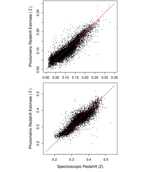
Figure 1: Top: predictions for 10,000 randomly selected objects in the MSG validation set, for $({\widehat{\epsilon}},{\widehat{m}})$ = (0.05,150). Bottom: same as top, for the LRG validation set, with $({\widehat{\epsilon}},{\widehat{m}})$ = (0.012,200). In both cases, we remove 5$\sigma$ outliers from the sample prior to plotting, thus the actual number of plotted points is 9,740 (top) and 9,579 (bottom).

Figure 2: Top Left: estimated bias ${\widehat{z}}-Z$ for MSG redshift estimates ${\widehat{z}}$, computed in bins of width $\Delta Z$ = 0.01 in the range $Z\in[0.01,0.25]$. Top Right: estimated standard deviation for MSG redshift estimates (normalized by $1+Z$). Middle Left and Right: same as top left and right, except for LRG redshift estimates in bins of width $\Delta Z$ = 0.02 in the range $Z\in[0.20,0.44]$. Bottom Left and Right: same as top left and right, except for DEEP2 redshift estimates (ZQUALITY = 4) in bins of width $\Delta Z$ = 0.05 in the range $Z\in[0.0,1.5]$.

We determine estimator bias by binning the predictions ${\widehat{z}}$ as a function of $Z$, then in each bin computing $\bar{\widehat{z}}-Z$, with $\bar{\widehat{z}}$ being a 10% trimmed mean. See the top left panel of Fig. 2. It is readily apparent that there is a downward slope in the bias (i.e., redshifts are overestimated at low $Z$, and underestimated at high $Z$). This is not caused by model bias (a bias that one would mitigate by adding complexity to the model, e.g., changing from linear to quadratic regression), but rather by attenuation bias, in which measurement error (i.e., uncertainty in the predictor, in this case the diffusion coordinates) reduces the slope of the regression line (see Fig. 3; see also, e.g., Carroll et al. 2006).

Figure 3: Simple demonstration of the effect of attenuation bias on linear regression. Left: example of linear regression fit to data with no measurement error in the predictor and with response $Y\sim N(x,0.04)$, where $x=\{1,2,3,4\}$, i.e., each value of $Y$ is sampled from a Gaussian distribution with mean $x$ and variance 0.04. The black dots indicate the observed data, while the open circles show the true $(x,y)$ values. Right: same as left, but with measurement error applied to the predictor: $X\sim N(x,1)$. The effect of this measurement error is to reduce the slope of the regression line, on average. The mean reduction in slope for this toy example is 0.25 (from 1 to 0.75), as estimated via 10,000 simulations.

To demonstrate that our data are affected by attenuation bias, we perform a simple experiment. First, we take the MSG training set fluxes and resample them according to the prescription given in Appendix B. This increases all measurement errors. (To see this intuitively, imagine sampling random variables $X\sim N(0,1)$, i.e., each value of $X$ is sampled from a Gaussian distribution with mean 0 and variance 1. Then resample from the observed values $X$: $Y\sim N(X,1)$. The standard deviation of the resulting sample is now $\sqrt{2}$, i.e., the error has been artificially increased by resampling.) Then we resample fluxes for 1,000 randomly selected validation set objects. By doing each resampling (training set and validation set) 25 times, we build up a set of 625 predictions of ${\widehat{z}}$ for each of the 1,000 selected objects. Following the same prescription as above, we estimate the bias; the top panel of Fig. 4 shows how for the MSG dataset, increasing the measurement error via resampling leads to a steepening of the bias slope, i.e., the effect of attenuation bias is magnified.

There exist methods for correcting the bias in linear regression coefficient estimation caused by additive, heteroscedastic (i.e., non-constant) measurement errors of known magnitude that are based on the SIMEX, or simulation-extrapolation, algorithm (Cook & Stefanski 1994; see, e.g., Carroll et al. 2006 and references therein). Indeed, one of the advantages to our approach is that the non-linearity is in the reparametrization, not the fitted model. Hence, available methods for correcting for measurement error could be utilized. We are currently exploring the implementation of SIMEX-based methods in a computationally efficient manner, and we will present our results in a future publication.

Figure 4: Top: change in the estimated bias ${\widehat{z}}-Z$ induced by resampling MSG training and validation set fluxes and refitting. Because resampling increases the measurement error (i.e., the error in the predictor, in this case the diffusion coordinates), the slope of the regression line is reduced, increasing overestimates of ${\widehat{z}}$ at low $Z$ and underestimates of ${\widehat{z}}$ at high $Z$. Bottom: same as top, for LRG datasets.

While attenuation bias is caused by measurement error, its magnitude is affected by the distribution of the predictors, i.e., the design. Expressions relating the design to the bias magnitude are highly problem dependent. In the simplest, one-dimensional example of attenuation bias, the predictors are assumed to be normally distributed–$X\sim N(\mu_{x},\sigma_{x}^{2})$–and the effect on the slope $\beta_{1}$ is to reduce its value: $\hat{\beta_{1}}\rightarrow\lambda\beta_{1}$, where $\lambda=\sigma_{x}^{2}/(\sigma_{x}^{2}+\sigma_{u}^{2})$ and $\sigma_{u}$ is the measurement error. The smaller the value of $\sigma_{x}^{2}$, the greater the effect upon the bias. We mention this explicitly to underscore that analyzing samples for which the predictors are, e.g., uniformly distributed may reduce the magnitude of the bias magnitude but will not eliminate it since measurement error is still present. In Fig. 5, we show the estimated sample bias as a function of $Z$ for a 10,000-galaxy sample constructed so as to be uniform in $Z$ (though the distribution of the predictors themselves–the diffusion coordinates–is not necessarily uniform). Comparing these results with the top panels of Fig. 2, we find that uniformity in $Z$ reduces the bias slightly (while also slightly increasing sample standard deviation). This indicates that measurement error is the dominant cause of the observed bias.

Figure 5: Left: estimated bias ${\widehat{z}}-Z$ for MSG redshift estimates ${\widehat{z}}$, computed in bins of width $\Delta Z$ = 0.01 in the range $Z\in[0.01,0.25]$, for a 10,000-galaxy sample constructed so as to be uniform in $Z$. Uniformity in $Z$ reduces the bias slightly (cf. the top panel of Fig. 2). This result indicates that measurement error is the dominant cause of the bias. Right: estimated standard deviation for MSG redshift estimates (normalized by $1+Z$).

Nonparametric estimators such as k-nearest neighbor (kNN) and local polynomial regression are also affected by measurement error bias (whose mitigation is dubbed the “deconvolution problem”) and design bias, and in addition by boundary bias (see, e.g., chapter 5 of Wasserman 2006 and chapter 12 of Carroll et al. 2006 and references therein). Thus the similarity of our bivariate distribution to that of, e.g., Ball et al. (See their fig. 6. In this figure, we note slightly larger deviations from the $\hat{z}=Z$ locus at the endpoints than our bivariate distribution exhibits, which may indicate boundary bias but also could be a result of the fact that Ball et al. do not minimize risk and thus could be adopting a solution with relatively higher bias and lower variance than our solution.)

In addition to estimator bias, we also examine the estimator variance, i.e., the width of the observed bivariate distribution (given as a function of $Z$ in the right column of Fig. 2). Contributing to the variance is (a) model uncertainty, i.e., the standard deviation of the estimates ${\widehat{z}}$ (given by the square root of the diagonal elements of the matrix given in equation 12); (b) uncertainty in the flux for each object; and (c) intrinsic scatter, i.e., the fact that the MSG sample does not necessarily contain a homogeneous set of objects. Model uncertainty contributes little to the observed scatter; the mean, median, and standard deviation of the model uncertainties are $\la$ 10^-5. Flux uncertainty enters via attenuation bias; as flux errors increase, the linear regression slope flattens and acts to decrease the sample variance within a redshift bin. However, in our simple attenuation-bias demonstration we observe only negligible changes in the sample variance. Thus we conclude that the observed sample variance is primarily due to intrinsic scatter, and can only be reduced by introducing more data (cf. Ilbert et al. 2008, who achieve ${\widehat{R}}_{CV}\la$ 0.01 by utilizing data from 30 bands in the UV, optical, and IR regimes).

3.1.2 Luminous red galaxies

From our data sample, we extract those 30,700 galaxies for which $Z>0.2$ and PRIMTARGET = 32 (TARGETGALAXYRED; Eisenstein et al. 2001). This is our luminous red galaxy or LRG sample. As with the MSG training set, we randomly select 10,000 galaxies and then remove outliers. Because the $u$ band data of high-redshift LRGs lacks constraining power (as LRGs are faint in $u$ and thus the magnitudes are noisy), we use only $griz$ fluxes in analyses (so that $p$ = 12). The training set contains 9,734 objects. Application of the algorithm outlined in §§2.1-2.2 yields tuning parameter estimates $({\widehat{\epsilon}},{\widehat{m}})$ = (0.012,200). The results of fitting are shown in Table 1 and the bottom panel of Fig. 1. As in the case of the MSG analysis, our value ${\widehat{R}}_{CV}$ = 0.0195 (0.0270 without $1+Z$ normalization) compares favorably with, e.g., Ball et al. 2008, who achieve $\sigma$ = 0.0242 (without $1+Z$ normalization), and references therein. We find that the outlier rate is consistent from training set to validation set (increasing from 2.7% to 3.1%), and that ${\widehat{R}}_{CV}$ increases by only 3.1% when we use the Nyström extension as opposed to directly fitting the data. (Note that if we include the $u$ band, the estimate of ${\widehat{\epsilon}}$ increases by two orders of magnitude, indicating the scatter in colour space introduced by non-constraining $u$-band data, although ${\widehat{R}}_{CV}$ itself only rises by $\approx$ 5%.) The LRG redshift predictions, like their MSG counterparts, are biased, with a similar downward trend in the bias as a function of $Z$ (left middle panel, Fig. 2). We repeat our simple resampling experiment with LRG data and find that the bias slope increases upon resampling, demonstrating that attenuation bias also affects LRG data analysis (as expected; see Fig. 4).

3.2 DEEP2/CFHTLS data

The DEEP2 Galaxy Redshift Survey (Davis et al. 2003, Davis et al. 2007) studied both galaxy properties and large-scale structure primarily at redshifts $0.7\la z\la 1.4$, in four fields of total area $\sim$ 3 square degrees. DEEP2 targets are selected to have $R_{AB}\leq$ 24.1 using CFHT BRI photometric data (Coil et al. 2004). In three of the four DEEP2 fields, colour cuts are used to select $z>$ 0.7 objects for observation; however, in this paper we utilize the DEEP2 sample in the Extended Groth Strip, for which no colour cuts have been applied. DEEP2 collected spectra typically covering the wavelength range 6,500$-$9,100 Å for $>$ 50,000 objects. From the survey we select the 6,552 galaxies for which single-system $ugriz$ photometry exists from the CFHT Legacy Survey (field D3) and for which the DEEP2 ZQUALITY flag is either 3 or 4 ($>$ 95% or 99.5% confidence that the redshift is correct, respectively). Thus the dimensionality of colour-space for these data is $p$ = 4. We further remove data for which the redshift error, or any magnitude or magnitude error, is not provided, leaving 6,418 galaxies; after outlier removal, the final sample size is 6,067. If we restrict ourselves to data for which ZQUALITY = 4, the sample size is 5,223.

Application of the algorithm outlined in §§2.1-2.2 yields tuning parameter estimates $({\widehat{\epsilon}},{\widehat{m}})$ = (0.002,850) for ZQUALITY = 4 and (0.002,1050) for ZQUALITY $\geq$ 3. We display our results in Table 1 and Fig. 6; note that because we do not apply the Nyström extension here (but rather, fit to the data directly after $({\widehat{\epsilon}},{\widehat{m}})$ are determined), the observed scatter is smaller than we would observe with a larger, Nyström-extended dataset. In both cases, we exclude 5.8% of the objects from analysis as outliers.

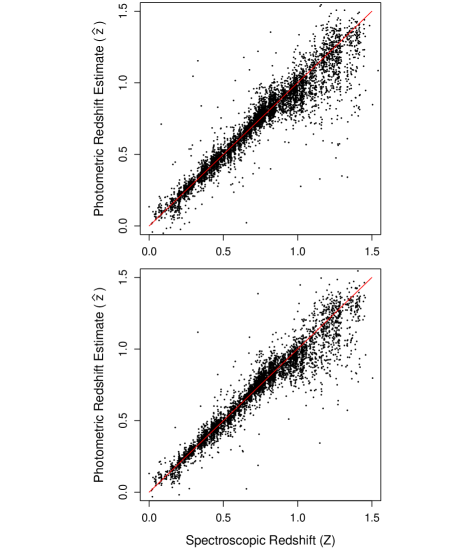
Figure 6: Top: predictions for the 6,067 objects in the DEEP2 training set for which ZQUALITY $>$ 3. For these data, $({\widehat{\epsilon}},{\widehat{m}})$ = (0.002,1050) and ${\widehat{R}}_{CV}$ = 0.0539. Bottom: same as top, for the 5,223 objects for which ZQUALITY = 4; $({\widehat{\epsilon}},{\widehat{m}})$ = (0.002,850) and ${\widehat{R}}_{CV}$ = 0.0507.

In Fig. 6, we observe that the quality of the fits below $Z\approx$ 0.75 (${\widehat{R}}_{CV}$ = 0.038 for ZQUALITY = 4) is superior to that at higher redshifts (${\widehat{R}}_{CV}$ = 0.064). To understand why this is so, we examine the DEEP2 colour data (Fig. 7).

Figure 7: Observed $ugriz$ colours for the 5,223 objects in the DEEP2 training set for which ZQUALITY = 4.

Pick an object at $Z\approx 0.75$, and compute the Euclidean distance in colour-space to a random object at any other redshift $Z\in[0,1.5]$. This distance is a nearly constant function of $\Delta Z$; thus for values of $\epsilon$ similar to those chosen in the SDSS analyses, there is only a slightly lesser probability of diffusing from $Z=$ 0.75 to, e.g., $Z=$ 0.2 as to, e.g., $Z=$ 0.74. To achieve accurate predictions at $Z\approx 0.75$, $\epsilon$ must be made smaller (lessening the probability of large $\Delta Z$ jumps); this is what our optimization yields. A consequence of a smaller ${\widehat{\epsilon}}$ is that the weighted graph of the DEEP2 objects is not fully connected (see discussion around equation 1). One can discern connectedness by examining the vector of eigenvalues; for ${\widehat{\epsilon}}$ = 0.002, the first $\approx$ 20 eigenvalues are all $>$ 0.95, implying the presence of several disconnected clumps on the graph. The most visually obvious manifestation of disconnectedness in the DEEP2 analysis is the presence of a marked knee in the predictions at $Z\approx$ 0.75 for small values of $m$ (see Fig. 8); the dominant eigenvectors describe the low redshift data well, but not the high redshift data.

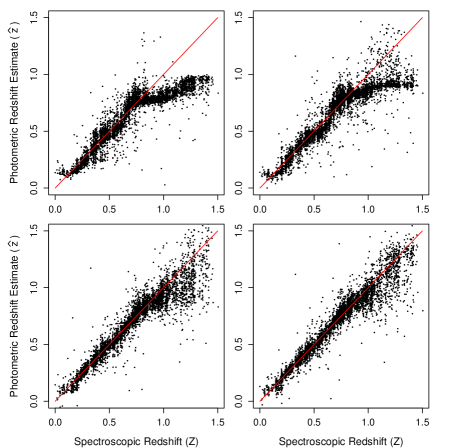
Figure 8: Predictions for the 5,223 objects in the DEEP2 training set for which ZQUALITY = 4, for ${\widehat{\epsilon}}$ = 0.002 and $m$ = 40 (top left), 100 (top right), 400 (bottom left), and 850 (${\widehat{m}}$; bottom right).

As $m$ increases, the knee straightens out; however, because of the bias-variance tradeoff, $m$ can only increase so much before ${\widehat{R}}_{CV}$ begins to increase as well, due to increasing variance. For ${\widehat{m}}$ = 850 (ZQUALITY = 4) we have not yet achieved an optimal description for the high-redshift data. To demonstrate that we can achieve a better description of these data, we split the full dataset into low- and high-redshift sets (at, e.g., $Z_{\rm cut}$ = 0.9) and compute diffusion maps for each. We find that we can achieve, e.g., ${\widehat{R}}_{CV}\approx$ 0.035 for high-redshift data with as few as 40 eigenvectors, while the predictions at low redshifts change only slightly. While splitting the data yields better results for our DEEP2 sample, we do not propose such splitting as part of our general diffusion map framework, for multiple reasons: (a) it adds a tuning parameter ($Z_{\rm cut}$), (b) it complicates the Nyström extension (to which data split do we assign a new object?), and most importantly (c) a data split can be rendered moot with the inclusion of new data in other bandpasses (e.g., the inclusion of near-IR data in the DEEP2 sample would mitigate the Euclidean-distance issue seen at $Z\approx 0.75$).

Concentrating on the regime $Z\la 0.75$, we find that our result ${\widehat{R}}_{CV}\approx 0.035$ with $\eta\approx$ 1.1% compares favorably with that of Ilbert et al. (2006), who train a template-based photometric redshift code using 2,867 spectroscopic redshifts from the VIMOS VLT Deep Survey (VVDS) in the CFHTLS D1 field and obtain $\sigma=0.032$ and $\eta=$ 4% (see their §6.3 and fig. 14). Our smaller catastrophic failure rate is presumably largely due to our removal of colour-space outliers prior to analysis. We note that Ilbert et al. perform a similar analysis with CFHTLS $z$-band data removed, with the result that a marked knee appears at $Z\approx$ 0.8 that is similar to what we observe in analyzing our intrinsically bluer DEEP2 sample. This supports the hypothesis that adding data from other bandpasses to our DEEP2 sample will lead to a marked improvement in fit at redshifts $Z\ga$ 1.

4 Summary and future directions

In this paper we apply an eigenmode-based framework utilizing the diffusion map and linear regression to the problem of estimating redshifts given SDSS and DEEP2/CFHTLS $ugriz$ photometry. Because estimating diffusion map coordinates via eigen-decomposition limits the size of training sets to $\sim$ 10⁴ objects, we implement the Nyström extension, which allows for computationally efficient estimation of diffusion coordinates with a relatively small degradation of accuracy.

For our SDSS MSG sample, we train our linear regression model on 9,749 randomly selected objects and via the Nyström extension estimate redshifts for another 340,989 galaxies. Since the Nyström extension is not robust to extreme outliers, we use a nearest-neighbor algorithm to eliminate 5$\sigma$ outliers in colour space; this eliminates $\approx$ 2.5% of the MSG sample. The loss in accuracy resulting from use of the Nyström extension is $\approx$ 2.4% (as compared with directly fitting the data of the training set). For our SDSS LRG sample, we train our regression model on 9,734 objects and via the Nyström extension estimate redshifts for another 20,082, with an outlier rate $\approx$ 3% and a degradation of accuracy $\approx$ 3%. As the DEEP2/CFHTLS sample has only $\approx$ 6,000 objects (with an outlier rate of $\approx$ 5.8%), we do not define a validation set to check the accuracy of predictions generated via the Nyström extension. However, we will apply our regression model to a test set comprised of all galaxies in CFHTLS fields D1-D4 and make that catalog publicly available.

The observed bivariate distributions $({\widehat{z}},Z)$ for our SDSS datasets are similar to those computed by, e.g., Collister & Lahav (2004) using ANNz (specifically, for the SDSS MSG dataset) and by Ball et al. (2008) using a numerically intensive nearest-neighbor algorithm (for both the SDSS MSG and LRG datasets), with dispersion on par with those techniques (${\widehat{R}}_{CV}\sim 0.02$; see Ball et al. 2008 and references therein). These distributions indicate that redshifts are generally overestimated at low $Z$ and underestimated at high $Z$. We demonstrate that this is a manifestation of attenuation bias, wherein measurement error (uncertainty in the diffusion coordinates resulting from uncertainty in the SDSS flux estimates) reduces the measured slope of the regression line. In statistical parlance, the measured slope is not a consistent estimator of the true slope. In order to use photometric redshift estimates in precision cosmology, it is vital that methods for producing consistent estimates (i.e., mitigating the bias) be developed and implemented. We are exploring using the SIMEX, or simulation-extrapolation, algorithm (e.g., Carroll et al. 2006) to produce consistent estimates in a computationally efficient manner, and we will present our results in a future publication.

For the DEEP2 data, the dominant feature in the observed bivariate distribution, beyond attenuation bias, is a marked reduction in prediction accuracy at redshifts $Z\ga$ 0.75. We demonstrate that this is due to a degeneracy in the colour-space manifold that would be mitigated with the introduction of more data from other bandpasses. We note that we also can mitigate the effects of the degeneracy by splitting the training set into low- and high-$Z$ samples, but we do not prefer this approach because of the complexity it adds to the prediction algorithm (through the addition of a tuning parameter $Z_{\rm cut}$ and the necessity of providing a quantitative measure for robustly choosing between the two predictions we would generate for each test object). At lower redshifts, we find that the observed bivariate distribution $({\widehat{z}},Z)$ compares favorably with that derived by Ilbert et al. (2006) (${\widehat{R}}_{CV}\approx$ 0.035 versus $\sigma$ = 0.032).

Our current statistical framework yields a single photometric redshift estimate for each object in the validation set, as opposed to a probability distribution function (PDF) for each estimate (cf. Ball et al. 2008). This is a valid approach for analyzing, at the very least, the galaxies of the SDSS sample that we consider in this work, as Ball et al. demonstrate that the PDFs in the low-redshift regime are approximately normal; we expect our single estimates to match the PDF means. However, we would have to alter our framework if we were to analyze quasars, for which the PDFs are often bimodal (e.g., fig. 5 of Ball et al.). Bimodality is an indication of (near-)degeneracy in the colour-space manifold; when its colours are perturbed, a quasar’s nearest neighbor sometimes belongs to one range of redshifts, and sometimes to a completely different range. Within our current framework, such a degeneracy would not affect the computation of the diffusion map, but the subsequent application of linear regression would yield inaccurate redshift estimates for those quasars in the vicinity of the degeneracy. For quasar analysis, we would explore a variety of options, which include (a) utilizing a different form of regression, (b) incorporating the response variables into the construction of the diffusion map (Costa & Hero 2005), and/or (c) incorporating gradient information into diffusion map construction, such that nearby objects that lie along the manifold have higher similarity measures. Such schemes would mitigate but not entirely lift the degeneracy and thus we would also have to quantify the relative probabilities of dual estimates.

In this work, we demonstrate the efficacy of SCA, in particular our diffusion map framework, for analyzing datasets for which the spectroscopic redshifts are known. The next step is to extend our framework such that it yields accurate photometric redshift estimates for objects in datasets where the spectroscopic coverage will be minimal, such as deep sky surveys (e.g., LSST) or pointed surveys beyond $Z\approx 1$. Even with long exposure times, the DEEP2 Galaxy Redshift Survey is only able to determine secure redshifts for $\sim$ 70% of its objects, with about half the missed targets being star-forming galaxies at $Z>1.4$ that have no features in DEEP2 spectral window; cf. Cooper et al. (2006). Even when spectroscopic redshifts are available for a significant subset of these objects, it is likely that they will be gleaned from intrinsically luminous objects whose SEDs may not closely match those for fainter objects. Thus it becomes imperative to fold additional information into analyses. Collister & Lahav (2004), Ball et al. (2004), and Wray & Gunn (2008) propose using structural properties such as surface brightness and angular radius to obtain more accurate redshift estimates; however, this is of limited utility at higher redshifts. Newman (2008) proposes that photometric redshifts can be calibrated using their correlations on the sky with objects of known redshift, as a function of that known redshift. A related idea would be to take into account the redshifts of nearby objects on the sky in estimating photometric redshifts (Kovac et al. 2009); because of the clustering of galaxies, there is a significant probability that two galaxies near each other on the sky are at very similar redshifts.

In a future work, we will fold additional quantities into our similarity measure and will determine if photometric redshift can be estimated with sufficient accuracy so as to fulfill their promise as a cosmological probe.

Appendix A Relevant formulae for weighted linear regression

Let X represent a matrix of predictors (in this work, the matrix of diffusion coordinates $\mathbf{\Psi}$, where each row represents the coordinates for a single object), let $Y$ represent the vector of responses (the estimated spectroscopic redshift values), and let $\mathbf{\Sigma}$ represent the covariance matrix for $Y$, which we assume to be diagonal:

$$\mathbf{\Sigma}=\left(\begin{array}[]{cccc}s_{Z_{1}}^{2}&0&\cdots&0\\ 0&s_{Z_{2}}^{2}&\cdots&\vdots\\ \vdots&\vdots&\vdots&\vdots\\ 0&\cdots&\cdots&s_{Z_{n}}^{2}\end{array}\right)\,,$$ (9)

Then the best-fit coefficients are

$${\widehat{\beta}} = \textbf{{A}}Y$$ (10)

$$= \left(\textbf{{X}}^{T}\mathbf{\Sigma}^{-1}\textbf{{X}}\right)^{-1}\textbf{{X}}^{T}\mathbf{\Sigma}^{-1}Y\,,$$

the variance-covariance matrix for $\widehat{\beta}$ is

$$\mathbb{V}({\widehat{\beta}}) = \mathbb{V}(\textbf{{A}}Y)$$ (11)

$$= \textbf{{A}}\mathbb{V}(Y)\textbf{{A}}^{T}$$

$$= \left(\textbf{{X}}^{T}\mathbf{\Sigma}^{-1}\textbf{{X}}\right)^{-1}\textbf{{X}}^{T}\mathbf{\Sigma}^{-1}\mathbb{V}(Y)\mathbf{\Sigma}^{-1}\textbf{{X}}\left(\textbf{{X}}^{T}\mathbf{\Sigma}^{-1}\textbf{{X}}\right)^{-1}$$

$$= \left(\textbf{{X}}^{T}\mathbf{\Sigma}^{-1}\textbf{{X}}\right)^{-1}\textbf{{X}}^{T}\mathbf{\Sigma}^{-1}\textbf{{X}}\left(\textbf{{X}}^{T}\mathbf{\Sigma}^{-1}\textbf{{X}}\right)^{-1}$$

$$= \left(\textbf{{X}}^{T}\mathbf{\Sigma}^{-1}\textbf{{X}}\right)^{-1}$$

and the variance-covariance matrix for $\widehat{Y}=\textbf{{X}}{\widehat{\beta}}$ is

$$\mathbb{V}({\widehat{Y}}) = \mathbb{V}(\textbf{{X}}{\widehat{\beta}})$$ (12)

$$= \textbf{{X}}\mathbb{V}({\widehat{\beta}})\textbf{{X}}^{T}$$

$$= \textbf{{X}}\left(\textbf{{X}}^{T}\mathbf{\Sigma}^{-1}\textbf{{X}}\right)^{-1}\textbf{{X}}^{T}\,.$$

Appendix B Resampling SDSS flux measurements

We assume each flux is a normal deviate with error estimated by the Princeton/MIT data reduction pipeline. However, fluxes in, e.g., different SDSS magnitude bands and systems are correlated random variables. In order to resample fluxes accurately, we must take these correlations into account. For each object in the validation set, we have 20 flux measurements $F$ and estimates of flux standard error $s_{F}$. The covariance matrix $\mathbf{\Sigma}$ is defined as

$$\mathbf{\Sigma}=\left(\begin{array}[]{cccc}1&\rho_{1,2}s_{F_{1}}s_{F_{2}}&\cdots&\rho_{1,20}s_{F_{1}}s_{F_{20}}\\ \rho_{1,2}s_{F_{1}}s_{F_{2}}&1&\cdots&\vdots\\ \vdots&\vdots&\vdots&\vdots\\ \rho_{1,20}s_{F_{1}}s_{F_{20}}&\cdots&\cdots&1\end{array}\right)\,,$$ (17)

where $\rho_{i,j}$ is the sample correlation coefficient between measurements $i$ and $j$ (e.g., between the PSF $u$-band and the Petrosian $r$-band). We estimate $\rho_{i,j}$ using Pearson’s product-moment correlation estimator

$$\rho_{i,j}=\frac{1}{n-1}\sum_{k=1}^{n}\left(\frac{F_{i,k}-{\bar{F}}_{i}}{s_{i}}\right)\left(\frac{F_{j,k}-{\bar{F}}_{j}}{s_{j}}\right)\,,$$

where $s$ is the sample standard deviation. As expected, we find that fluxes measured via different systems within a single magnitude band are strongly positively correlated ($\rho>0.5$); also, we find that fluxes across bands have non-negligible positive correlations, which we attribute to the relative homogeneity of the MSG sample (whose objects lie at relatively similar distances and display relatively similar physical characteristics). However, so as not to impose this homogeneity in resampling, we set $\rho_{i,j}$ = 0 if indices $i$ and $j$ represent different magnitude bands.

We use the Cholesky method to decompose $\mathbf{\Sigma}$ into lower- and upper-triangular matrices A and $\textbf{{A}}^{\rm T}$. Then we can compute a new vector of fluxes:

$$F_{i}^{\prime}=F_{i}+\textbf{{A}}z\,,$$

where $z$ is a vector of standard normal deviates.

References

- Albrecht et al. (2006) Albrecht A. et al. 2006, (preprint:astro-ph/0609591)
- Ball et al. (2004) Ball N. M. et al. 2004, MNRAS, 348, 1038
- Ball et al. (2007) Ball N. M. et al. 2007, ApJ, 663, 774
- Ball et al. (2008) Ball N. M., Brunner R. J., Myers A. D., Strand N. E., Alberts S. L., Tcheng D. 2008, ApJ, 683, 12
- Benítez (2000) Benítez N. 2000, ApJ, 536, 571
- Budavári et al. (2005) Budavári T. et al. 2005, ApJ, 619, L31
- Budavári et al. (2009) Budavári T., Wild V., Szalay A. S., Dobos L., Yip C.-W. 2009, MNRAS, 394, 1496 2005, ApJ, 619, L31
- Carroll et al. (2006) Carroll R., Ruppert D., Stefanski L., Crainiceanu C. 2006, Measurement Error in Nonlinear Models, Chapman and Hall, New York, NY
- Coifman & Lafon (2006) Coifman R. R., Lafon S. 2006, Appl. Comput. Harmon. Anal., 21, 5
- Coil et al. (2004) Coil A. L. et al. 2004, ApJ, 617, 765
- Collister & Lahav (2004) Collister A. A., Lahav O. 2004, PASP, 16, 345
- Connolly et al. (1995) Connolly A. J., Csabai I., Szalay A. S., Koo D. C., Kron R. G., Munn J. A. 1995, AJ, 110, 2655
- Cook & Stefanski (1994) Cook J. R., Stefanski L. A. 1994, JASA, 89, 1314
- Cooper et al. (2006) Cooper M. C. et al. 2006, MNRAS, 370, 198
- Costa & Hero (2005) Costa J. A., Hero A. O. 2005, ICASSP, 5, 1077
- Davis et al. (2003) Davis M. et al. 2003, SPIE Proceedings, 4834, 161
- Davis et al. (2007) Davis M. et al. 2007, ApJ, 660, L1
- Eisenstein et al. (2001) Eisenstein D. J. et al. 2001, AJ, 122, 2267
- Feldmann et al. (2006) Feldmann R. et al. 2006, MNRAS, 372, 565
- Fernández-Soto, Lanzetta, & Yahil (1999) Fernández-Soto A., Lanzetta K. M., Yahil A. 1999, ApJ, 513, 34
- Finkbeiner et al. (2004) Finkbeiner D. P. et al. 2004, AJ, 128, 2577
- Gwyn (2008) Gwyn S. D. J. 2008, PASP, 120, 212
- Ilbert et al. (2006) Ilbert O. et al. 2006, A&A, 457, 841
- Ilbert et al. (2008) Ilbert O. et al. 2008, ApJ, 690, 1236
- Ivezić et al. (2008) Ivezić Ž et al. 2008, (preprint:arXiv/0805.2366)
- Kovac et al. (2009) Kovac K. et al. 2009, BAAS, 41, 378
- Lafon & Lee (2006) Lafon S., Lee A. 2006, IEEE Trans. Pattern Anal. and Mach. Intel., 28, 1393
- Lee & Wasserman (2009) Lee, A., Wasserman, L. 2009, JRSS B, submitted (preprint:arXiv/0811.0121)
- Ma, Hu, & Huterer (2006) Ma Z., Hu W., Huterer D. 2006, ApJ, 636, 21
- Newman (2008) Newman J. A. 2008, ApJ, 684, 88
- Oyaizu et al. (2008) Oyaizu H., Lima M., Cunha C. E., Lin H., Frieman J., Sheldon E. S. 2008, ApJ, 674, 768
- Padmanabhan et al. (2008) Padmanabhan N. et al. 2008, ApJ, 674, 1217
- Press et al. (1992) Press W., Teukolsky S., Vetterling W., Flannery B., Numerical Recipes in C, Cambridge Univ. Press, Cambridge
- Richards et al. (2009a) Richards J. W., Freeman P. E., Lee A. B., Schafer C. M. 2009, ApJ, 691, 32
- Richards et al. (2009b) Richards J. W., Freeman P. E., Lee A. B., Schafer C. M. 2009, MNRAS, submitted (preprint:arXiv/0905.4683)
- Strauss et al. (2002) Strauss M. A. et al. 2002, AJ, 124, 1810
- Vanzella et al. (2004) Vanzella E. et al. 2004, A&A, 423, 761
- Wasserman (2006) Wasserman L. W. 2006, All of Nonparametric Statistics, Springer, New York, NY
- Wray & Gunn (2008) Wray J. J., Gunn J. E. 2008, ApJ, 678, 144