Binary orbit, physical properties, and evolutionary state of Capella ($\alpha$ Aurigae)

Abstract

We report extensive radial-velocity measurements of the two giant components of the detached, 104-day period binary system of Capella. Our highly accurate three-dimensional orbital solution based on all existing spectroscopic and astrometric observations including our own yields much improved masses for the primary and secondary of $2.466\pm 0.018~{}M_{\sun}$ and $2.443\pm 0.013~{}M_{\sun}$, with relative errors of only 0.7% and 0.5%, respectively. The mass ratio is considerably closer to unity than previously believed, which has an impact on assessing the evolutionary state of the system. Improved values are presented also for the radii ($11.87\pm 0.56~{}R_{\sun}$ and $8.75\pm 0.32~{}R_{\sun}$), effective temperatures ($4920\pm 70$ K and $5680\pm 70$ K), and luminosities ($79.5\pm 4.8~{}L_{\sun}$ and $72.1\pm 3.6~{}L_{\sun}$). The distance is determined to be $13.042\pm 0.028$ pc, based on the accurate orbital parallax. The projected rotational velocities and individual rotation periods are also known. Capella is unique among evolved stars in that, in addition to all of the above, the chemical composition is known as well. This includes the overall metallicity [m/H], the carbon isotope ratio ¹²C/¹³C for the primary, and the lithium abundance and C/N ratios for both components. We present new or revised values for some of these. The latter three quantities are sensitive diagnostics of evolution, and change drastically for giants as a result of the deepening of the convective envelope during the first dredge-up. The secondary is crossing the Hertzprung gap, while the primary is believed to be in the longer-lived core-helium burning phase. Previous studies using only the masses, temperatures, and luminosities have found good agreement with stellar evolution models placing the primary in the clump. Here we compare all of the constraints simultaneously against three sets of current models. We find that they are unable to match all of the observations for both components at the same time, and at a single age, for any evolutionary state of the primary. This shows the great importance of chemical information for assessing the evolutionary state of giant stars. A comparison with models of tidal evolution yields similarly disappointing results, when tested against the fact that the orbit is circular, the primary is rotating synchronously, the secondary $\sim$12 times faster than synchronous, and the spin axes are apparently aligned with the axis of the orbit. When confronted in detail, our understanding of the advanced stages of stellar evolution is thus still very incomplete.

1. Introduction

Our knowledge of stellar evolution relies heavily on constraints provided by measurements of the physical properties of stars, particularly the mass. Eclipsing binaries have been our main source of accurate information for stars on the main sequence (masses, radii, effective temperatures, luminosities). The more advanced stages of evolution, after the central hydrogen is exhausted, are much less well understood than the main-sequence phase primarily because of poorer or less stringent constraints. Accurate masses are rarely available for normal giant stars, for practical reasons that are well known: it requires them to be in binaries, and it requires the orbits to be wide enough so that the components are detached (i.e., that they do not interact with each other in the sense of mass transfer). This in turn calls for sustained observations over long periods of time, often several years. The radial-velocity amplitudes are typically low, making the masses more difficult to measure accurately. Eclipses are also much less likely, robbing us in most cases of the possibility of determining the absolute radii directly.

While precious few normal giants or subgiants are known to be in eclipsing binaries (examples include AI Phe, TZ For, and the system OGLE 051019.64$-$685812.3 in the LMC; Andersen et al., 1988, 1991; Pietrzyński et al., 2009), non-eclipsing systems amenable to both spectroscopic and astrometric studies enabling accurate dynamical mass determinations are somewhat more common. A very prominent example of this class of objects is Capella ($\alpha$ Aurigae, HD 34029, HR 1708, HIP 24608, G8 III+G0 III, $P=104$ days), the 6th brightest star in the sky ($V=0.07$), and the first binary for which an astrometric orbit was determined interferometrically (Anderson, 1920; Merrill, 1922). Although other astrometric measurements have been gathered for Capella over the decades using a variety of techniques, those pioneering observations with the original Michelson interferometer on Mount Wilson have remained a critical component of the astrometric solution of the orbit, which until about 15 years ago contributed the dominant share of the uncertainty in the resulting masses. At that time Hummel et al. (1994) used the Mark III interferometer, also on Mount Wilson, to obtain measurements that are an order of magnitude more precise. As a result, our knowledge of the masses is now limited by the best-available spectroscopy (Barlow et al., 1993) rather than the astrometry, a somewhat embarrassing situation given the brightness of the object and its 100-year observational history. The masses are currently estimated to be $2.69\pm 0.06~{}M_{\sun}$ and $2.56\pm 0.04~{}M_{\sun}$ for the cooler primary and the secondary, respectively. Although these are seemingly quite precise ($\sim$2% relative errors), the accuracy is just as important, especially for giants. The predicted properties of stars from stellar evolution models in these rapid evolutionary stages are extremely sensitive to mass, and a 2% error makes a much larger difference than on the main sequence.

Systematic errors in the radial velocity measurements for the rapidly-rotating secondary of Capella are not easy to avoid, and as a result there have been persistent concerns in the literature about the accuracy of the mass ratio, which is very close to unity. This quantity has a significant impact on the precise evolutionary state inferred for the components. One of our motivations here is thus to provide a new, high-quality set of spectroscopic observations that more nearly matches the precision of the astrometric data of Hummel et al. (1994). We focus especially on the accuracy of the mass determinations, for the purpose of comparing with state-of-the-art stellar evolution models. Considerable effort is therefore invested in the inter-comparison of all available astrometric and spectroscopic observations, in order to properly understand the systematics. An additional goal of this work is to carry out a comprehensive analysis of all the data relevant for the determination of the evolutionary state of Capella, which has been a subject of debate for decades. The secondary is clearly crossing the Hertzprung gap, but the primary has been suggested to be either in the helium-burning clump or on the first ascent of the giant branch, usually based on partial information. This system is perhaps unique in that, in addition to the masses, effective temperatures, and luminosities that have been used previously for that purpose, a wealth of other information is available. This includes direct measurements of the angular diameters, various activity indicators in the optical, ultraviolet, and X rays, the projected rotational velocities as well as the rotation periods, the overall metallicity, and particularly the surface lithium abundance of both stars, the ¹²C/¹³C isotope ratio for the primary star, and the C/N abundance ratios. Chemical indicators such as these are crucial diagnostics of evolution because they change significantly in the giant phase, mainly during the first dredge-up. We bring all of these to bear here, for the first time. We wish to examine the effects of convection prescriptions in the models (mixing length, overshooting) as well as rotation, which has not previously been considered for this system. Furthermore, Capella is an important point of comparison with tidal evolution theory for evolved stars. This is because the primary has its rotation synchronized with the orbital motion while the secondary rotates 12 times faster than synchronous, despite the nearly identical masses, which are within 1% of each other. Thus another goal of this work is to use our newly derived accurate dimensions for the components to carry out a detailed check of current tidal theories and gauge our understanding of these processes.

Our new spectroscopic observations are presented in § 2, along with all historical radial-velocity measurements. The astrometric observations are discussed in § 3, and include long-baseline interferometry, speckle interferometry, and Hipparcos measurements. Our simultaneous orbital solution for Capella based on these two kinds of data is documented in § 4, with particular care given to possible systematic errors that might bias the masses. In § 5 and § 6 we collect all the information available on the relative brightness of the components and the angular diameters, which we use later to estimate effective temperatures and absolute radii. The chemical composition of Capella is discussed in § 7, and proves to be of critical importance for the analysis. The physical properties of the stars are then described in § 8. We present a detailed comparison of the absolute dimensions of Capella with stellar evolution theory in § 9, focusing on the determination of the evolutionary state of the stars. In the same section we carry out tests of current tidal theories. Finally, § 10 summarizes our main conclusions. Two appendices collect notes of interest on the astrometric observations for the benefit of future users, and a third contains a discussion of the coronal abundances of Capella that support the photospheric determinations.

2. Spectroscopic observations

The rich history of the radial-velocity measurements of Capella began more than a century ago with the pioneering efforts by the Greenwich and Potsdam astronomers (Gill, 1891; Vogel, 1891), and has been recounted previously by other authors (see, e.g., Barlow et al., 1993). More than a dozen semi-independent spectroscopic orbital solutions have been reported over the decades, based on data sets of greatly varying quality. Despite the brightness of the object, the radial velocity measurements of the rotationally broadened secondary component are not particularly easy, and have not always been possible in the past. As a result, there has been considerable debate about the mass ratio (see, e.g., Batten et al., 1991), which our analysis conclusively shows is near unity. Nevertheless, some of these historical data are still of value to improve the orbital period, so we describe them in some detail below and make use of them later. Our main observational contribution here is a large new set of high-quality velocity measurements for both components that provides more than a two-fold improvement in the precision of the velocity semi-amplitude of the primary, and a four-fold improvement for the secondary compared to the best existing determinations, by Barlow et al. (1993). These new data are described first.

2.1. New radial-velocity measurements

Spectroscopic observations of Capella were conducted at the Harvard-Smithsonian Center for Astrophysics (CfA) using the 1.5m Wyeth reflector at the Oak Ridge Observatory (Harvard, Massachusetts), beginning in 1996 October and continuing through 1999 November. An echelle spectrograph with a photon-counting intensified Reticon detector (Digital Speedometer; Latham, 1985, 1992) was used to record a single 45 Å echelle order centered at a wavelength of 5188.5 Å, featuring the gravity-sensitive lines of the Mg I b triplet. The resolving power provided by this setup is $\lambda/\Delta\lambda\approx 35,\!000$. One additional observation was gathered with a nearly identical system on the 1.5m Tillinghast reflector at the F. L. Whipple Observatory (Mount Hopkins, Arizona). Nominal signal-to-noise ratios per resolution element of 8.5 km s^-1 range from about 20 to 90, although for values much higher than 50 the limit is set by systematics from flat-fielding and not photon noise. With the inclusion of two archival observations made in 1986 February and March with the instrument at Oak Ridge, the total number of usable spectra is 162, collected over an interval of 13.8 years.

Radial velocities for both stars were derived using TODCOR, a two-dimensional cross-correlation technique introduced by Zucker & Mazeh (1994). This method uses two templates, one for each component of the binary, which we selected from a large library of synthetic spectra based on model atmospheres by R. L. Kurucz (see Latham et al., 2002). These templates have been calculated for a wide range of effective temperatures ($T_{\rm eff}$), surface gravities ($\log g$), rotational velocities ($v\sin i$ when seen in projection), and metallicities ([m/H]). Following Torres et al. (2002) the optimum templates for Capella were determined by means of extensive grids of cross-correlations with TODCOR, seeking to maximize the average correlation weighted by the strength of each exposure. The surface gravities were held fixed at preliminary values of $\log g=2.5$ and 3.0 for the primary and secondary, and the metallicity was initially assumed to be solar. As a result of this optimization we obtained by interpolation effective temperatures of $T_{\rm eff}^{\rm A}=4900\pm 100$ K and $T_{\rm eff}^{\rm B}=5710\pm 100$ K for the primary and secondary, respectively, along with projected rotational velocities of $v_{\rm A}\sin i=6.5\pm 1.0$ km s^-1 and $v_{\rm B}\sin i=36.0\pm 1.5$ km s^-1. Strictly speaking, the latter values are a measure of the total broadening of the spectral lines. We discuss these measures and compare them with others in § 8. We repeated these determinations assuming metallicities of [m/H] $=-1.0$, $-$0.5, and +0.5, but we found the average correlation values to be slightly lower than with solar metallicity, indicating a poorer match to the observed spectra. The templates adopted here are the ones in our library with parameters nearest to the values above: $T_{\rm eff}=5000$ K and 5750 K for the primary and secondary, and rotational velocities of 6 km s^-1 and 35 km s^-1, respectively. The radial velocities derived in this way have internal errors averaging 0.5 km s^-1 and 1.0 km s^-1 for the primary and secondary, but vary individually depending on the signal-to-noise ratio. In addition to the radial velocities, our spectra yield the light ratio at the mean wavelength of our spectra, $\ell_{\rm B}/\ell_{\rm A}=1.48\pm 0.05$. The difference in line blocking between the components has been accounted for, so that this represents a true flux ratio rather than a ratio between the continuum levels. The hotter star is thus brighter at $\sim$5200 Å.

The stability of the zero-point of the CfA velocity system was monitored by means of exposures of the dusk and dawn sky, and small systematic run-to-run corrections were applied in the manner described by Latham (1992). The zero point of the native CfA velocity system based on synthetic templates is very close to the absolute frame as defined by extensive observations of the minor planets in the solar system. The correction required to place our radial velocities on this absolute frame is $+0.139~{}{\rm km\thinspace s^{-1}}$ (Stefanik, Latham & Torres, 1999; Latham et al., 2002), and has not been applied to the measurements listed below.

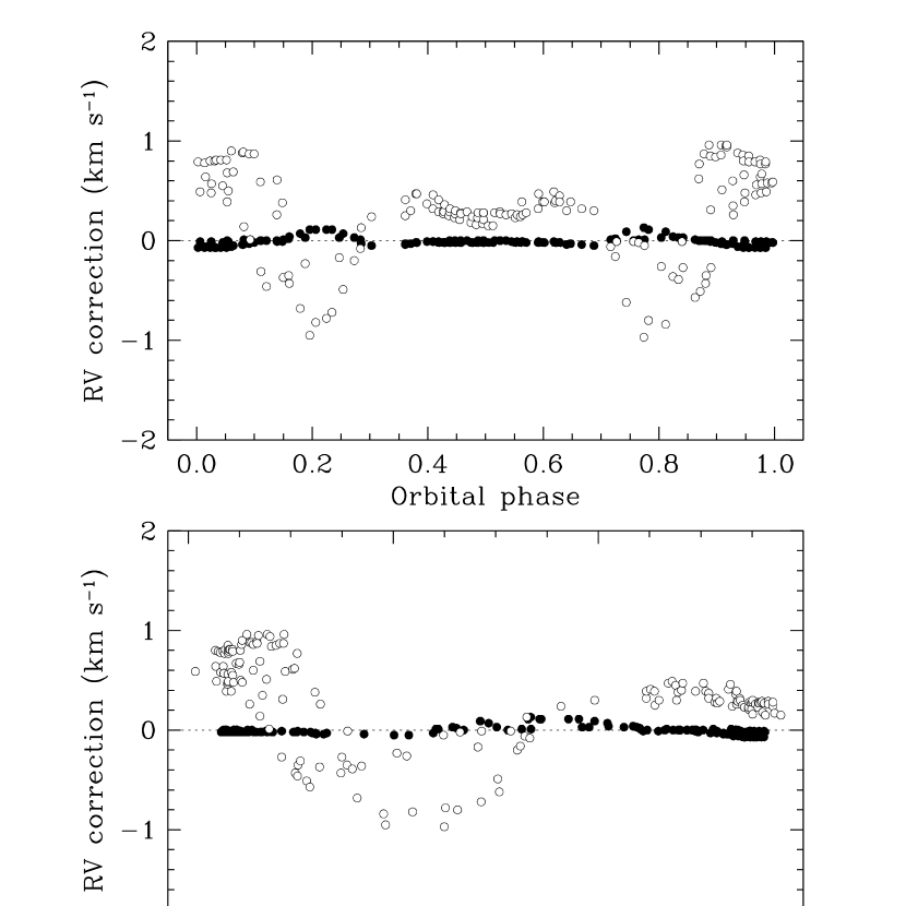
Figure 1.— Systematic errors in the raw TODCOR velocities for Capella as a function of orbital phase and velocity. Filled circles correspond to the primary, open circles to the secondary. These differences have been applied to the raw velocities as corrections (see text).

One of the main advantages of TODCOR compared to conventional one-dimensional cross-correlation techniques is that it greatly reduces the systematic errors in the radial velocities caused by line blending that have affected many of the previous studies of Capella (see § 2.2). Nevertheless, because we are concerned in this work with the accuracy of the velocities as much as their precision, we investigated possible systematic effects that may result from residual blending in our narrow spectral window, and from shifts of the spectral lines in and out of this window as a function of orbital phase. Previous experience with similar material has shown that these effects are sometimes significant, and must be examined on a case-by-case basis and corrected if necessary (see, e.g., Torres et al., 1997, 2000). We performed numerical simulations as described by Latham et al. (1996) to evaluate these effects. Briefly, we generated synthetic composite spectra matching our observations by combining the primary and secondary templates used above (including rotational broadening), shifted to the appropriate velocities for each of the exposures as predicted by a preliminary orbital solution, and scaled to the observed light ratio. These synthetic observations were then processed with TODCOR in exactly the same way as the real spectra, and the resulting velocities were compared with the input shifts. The differences are shown graphically in Figure 1, as a function of both velocity and orbital phase. The systematic pattern is obvious, and the individual differences can reach $\pm$1 km s^-1, which is relatively small in absolute terms but significant compared to the internal errors. We therefore applied these differences as corrections to the raw velocities. The effect on the primary semi-amplitude $K_{\rm A}$ is negligible, but the change in $K_{\rm B}$ is $\sim$0.5%, which translates into a non-negligible change in the derived masses of about 1% for the primary and 0.6% for the secondary. The final velocities in the heliocentric frame are given in Table 1, and include these corrections. Similar adjustments based on the same simulations were applied to the light ratio, and are already included in the value reported above.

Preliminary single-lined orbital solutions performed separately on the primary and secondary velocities indicated a slight difference in the center-of-mass velocities, $\gamma$, of about $0.27\pm 0.08$ km s^-1, with the secondary value being lower. Primary/secondary velocity differences considerably larger than this are not uncommon in studies of double-lined eclipsing binaries. This difference $\Delta_{\rm AB}$ persisted in our global solution described later. Although it is very small in absolute terms (only about half of the typical uncertainty in our primary velocities), it is statistically significant due to the large number of observations in the fit. Because it may affect the absolute masses of Capella at some level, we have explored possible reasons for this shift. One is the differential gravitational redshift between the stars, given that our synthetic templates do not account for this. Estimates based on preliminary values of the masses and radii of the components indicate that this effect is 0.046 km s^-1, but it goes in the wrong direction to explain $\Delta_{\rm AB}$, i.e., the secondary redshift is larger. It is also possible there are shifts due to large-scale convective motions (Schwarzschild, 1975; Porter & Woodward, 2000) that could be different in the two stars, but these are not well characterized for giants. Given that the stars are observed to be active, another possibility is the presence of spots on one or both components (particularly on the rapidly rotating secondary), which can affect the velocities. A perturbation of this nature was in fact pointed out by Hummel et al. (1994) for their interferometric visibilities of Capella (see § 4). Unfortunately our time sampling is inadequate to study this in more detail, but unless the spots are very long-lived we would expect the effect to average out to some extent over the interval of our observations. A fourth possibility that cannot be completely rule out is template mismatch (see, e.g., Griffin et al., 2000). We have made every effort here to use templates that maximize the average correlation for all our spectra, and small differences with the true values of $T_{\rm eff}$, $v\sin i$, $\log g$ (which we estimate below to be $\log g=2.68$ for the primary and 2.94 for the secondary) or metallicity compared to what we have assumed should not have a significant effect on the velocities, in our experience. However, line broadening from micro- or macro-turbulence in Capella could be somewhat different from what is assumed in our library of synthetic spectra (microturbulence $\xi_{\rm t}=2$ km s^-1 and macroturbulence $\zeta_{\rm RT}=1.5$ km s^-1), although this is unlikely to affect the secondary much due to the overwhelming effect of rotational broadening in that star (36 km s^-1). We discuss this effect further in § 9.2 in connection with the accuracy of the $v\sin i$ measurements. In the absence of a definitive explanation, we have chosen below to correct for the primary/secondary shift by solving for the offset and applying it to the secondary velocities. Not correcting for the shift would affect the semi-amplitudes at the level of 0.03% for the primary and 0.14% for the secondary, and the final masses at the level of 0.31% and 0.22%, which correspond to less than half of the formal uncertainties in our final determination of those quantities (see § 8).

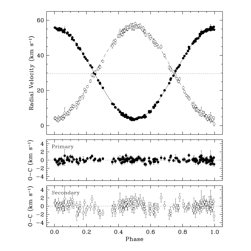
Figure 2.— CfA radial-velocity measurements for Capella (filled circles for the primary, open for the secondary) along with the curves computed from our combined orbital solution described in § 4. The dotted line represents the velocity of the center of mass. $O\!-\!C$ residuals for the primary and secondary are shown in the bottom panels.

Figure 2 displays the CfA observations along with an orbital solution described later, as well as the $O\!-\!C$ residuals. Those of the secondary show a small residual pattern which we believe to be of a similar nature as the $\Delta_{\rm AB}$ shift discussed above. We return to this later in connection with the orbital solution.

2.2. Historical radial-velocity measurements

The discovery of the binary character of Capella was announced independently by Campbell (1899) and Newall (1899) from photographic spectra taken at Lick Observatory and Cambridge Observatory (England), respectively. Both investigators noted the composite nature of the spectrum, but published velocities only for the component Newall referred to as being of “solar type”. In our nomenclature this is the cooler, slightly more massive star we refer to as the “primary” (star A), which has relatively sharp lines. The other star (of “Procyon type”, “secondary”, or star B) has much more diffuse lines. Campbell (1901) reported only that the velocity of the secondary varies between $-3$ km s^-1 and +63 km s^-1. His 31 measurements for the primary are of excellent quality ($\sigma_{\rm RV}\sim 0.8$ km s^-1), and were used by Reese (1900) to establish the first reliable spectroscopic orbit. The measurements by Newall (1900) are somewhat poorer ($\sigma_{\rm RV}\sim 2.1$ km s^-1), but still potentially useful.

The first published measurements of the secondary velocity appear to be those by Goos (1908), who succeeded in detecting it in 19 of his 35 photographic plates taken with a 0.3m refractor at Bonn. All plates yielded good measurements for the primary. Further velocities for both stars were reported by Sanford (1922) from Mount Wilson, and Struve (1939) from Babelsberg. Struve & Kilby (1953) published a further series of velocities from Mount Wilson and Lick, though only for the primary star. Measurements of the velocity difference between the components made at the Dominion Astrophysical Observatory (DAO) were reported by Wright (1954), along with a careful study of the secondary spectrum and the relative brightness of that star compared to the primary. The velocity measurements are averages from plates taken at similar orbital phases, so unique dates cannot be assigned to them and for this reason we do not use these data here. The brightness ratio as well as the mass ratio estimate by Wright (1954), derived by adopting the primary orbit from Struve & Kilby (1953), were quite influential over the following decades, although the light ratio is now known to be incorrect (or at least misleading; see § 5 and § 8). More recently Batten & Erceg (1975) published 18 velocities for the primary from plates obtained at DAO, most of which were later re-measured by Batten et al. (1991), superseding the original determinations. Further measurements for both components obtained at the Fick Observatory were reported by Shen et al. (1985). These data were in turn superseded and significantly expanded by Beavers & Eitter (1986), who published the largest set of velocities for Capella aside from our own. Additional measurements of the primary only were obtained by Shcherbakov et al. (1990), including a set based on photospheric lines and another set from the chromospheric He I $\lambda$10830 line. We do not use the latter because they may not correspond to the true center of mass of the star, nor do we consider a similar list of velocities for both components by Katsova & Scherbakov (1998), also from the He I $\lambda$10830 line. Finally, high-quality measurements for both stars from the McDonald and Kitt Peak Observatories were published by Barlow et al. (1993).

The sources above represent the most important velocity data sets published for Capella in the century since its discovery as a binary. Even though some of them may have considerably larger uncertainties (less weight) than the CfA velocities, in principle there is no reason why they cannot be properly combined with ours to strengthen the solution, which is our goal in § 4. A number of smaller lists of less than half a dozen measurements each have also appeared over the decades, but are ignored here for being much less significant and more difficult to use because of the poorly determined zero-point offsets. The richer sources are summarized in Table 2, where the last entry corresponds to our own contribution.

Figure 3.— Radial-velocity semi-amplitudes for the primary and secondary of Capella (filled and open circles, respectively) throughout the last century, based on our solutions in Table 2.

The potential usefulness of these historical data sets depends on whether they can be shown to be sufficiently free from systematic errors. To this end, we have examined each of the sources by computing separate orbital solutions from the original velocities with the same fitting code, and comparing them to one based on the CfA data. These solutions can be found in Table 2. We list also the number of observations, their time span, and the root-mean-square (RMS) residual from the fit in each case, which is representative of the typical error of the velocities. Because of the limited duration of some of these studies, the period has been held fixed at the value $P=104.022$ days determined from a preliminary fit to our own observations, and the orbit has been assumed to be circular. The center-of-mass velocities $\gamma$ in the second column show that there are occasional differences in the instrumental zero points, although these can easily be corrected in a combined solution by solving for the offsets simultaneously with the other adjustable parameters. The same holds for the primary/secondary offsets listed in the third column (see also § 2.1), which have been set to zero when a preliminary fit indicated the shift was not significant. We are more concerned here with the velocity semi-amplitudes $K_{\rm A}$ and $K_{\rm B}$, which determine the masses of the components. Excluding the two data sets that rely on chromospheric lines (Shcherbakov et al., 1990; Katsova & Scherbakov, 1998), the primary semi-amplitudes from all the others agree reasonably well with ours. The only exception is the data set by Sanford (1922), which is also the smallest. The secondary semi-amplitudes, however, show significant systematic differences with the CfA value of $K_{\rm B}$, and if we restrict ourselves to velocities based on photospheric lines, there appears to be a trend of decreasing amplitudes as a function of time over the last century, leading up to our own determination (see Figure 3). We suspect these differences have to do with systematic effects associated with line blending and the difficulty of measuring the broad spectral features of the secondary, particularly in the older studies, a problem that has been pointed out repeatedly over the years. For this reason, we have chosen not to use any of the historical secondary velocities here, relying only on our own. The primary velocities, on the other hand, appear reasonably free from systematics (save those of Sanford, 1922, which we exclude), and add up to more than twice the number of our own observations although the combined weight is actually $\sim$50% lower.

Figure 4.— Historical radial-velocity measurements for the primary component of Capella, along with the curve computed from our combined orbital solution described in § 4. Individual data sets have been placed on the same zero-point as the CfA velocities by applying the offsets described in § 4. The dotted line represents the velocity of the center of mass. $O\!-\!C$ residuals are shown in the bottom panel.

All of these velocities are listed in Table Binary orbit, physical properties, and evolutionary state of Capella ($\alpha$ Aurigae) on their original scales (i.e., without the application of any offsets, to be described below). Individual uncertainties are described in § 4. These observations are shown graphically in Figure 4, along with the same curve for the primary from Figure 2.

3. Astrometric observations

Soon after the discovery that Capella is a spectroscopic binary, some of the most skilled double-star observers of the day attempted to resolve the pair at the times predicted from the spectroscopic orbit to be the most favorable, but they were unsuccessful (Hussey, 1900; Aitken, 1900; Hussey, 1901). At about the same time, an intriguing series of visual measurements was made at the Greenwich Observatory that did appear to barely resolve the object: the observers reported elongated images with the 28-inch refractor. Systematic measurements of the position angle of the binary from these elongated images were carried out over an interval of about two years, and rough estimates of the angular separation were also made on a few occasions even though it was far smaller than the resolving power of the telescope. However, these observations were never confirmed and have been called into question, so we do not use them in our analysis. Nevertheless, a number of fascinating aspects of this puzzling data set are worth noting and are described in more detail in Appendix A.

It was not until 1919 that Capella was resolved in earnest, with the 6-m baseline Michelson interferometer on the 100-inch telescope on Mount Wilson (Anderson, 1920; Merrill, 1922). These pioneering observations are of high quality and internal consistency and have since been used in nearly all of the astrometric orbital solutions published for the system. They are valuable because of the extended time baseline they afford. We incorporate them into our own analysis as well, although they do contain some systematic errors that we address later. Except for two more recorded attempts by Wilson (1939, 1941) to resolve the pair visually, almost 50 years elapsed until the next astrometric observations were made at Pulkovo Observatory by Kulagin (1970), with a similar interferometer also using a 6-m baseline. Additional long-baseline interferometric observations have been reported by Blazit et al. (1977a) (baseline 12–20 m), Koechlin et al. (1979) (baseline 13.8 m), Koechlin et al. (1983) (baseline 5.5–35 m), Baldwin et al. (1996) (three-element Cambridge Optical Aperture Synthesis Telescope, COAST, using baselines up to 6.1 m), and more recently by Kraus et al. (2005) (three-element Infrared Optical Telescope Array, IOTA, using baselines up to 38 m). By far the most precise interferometric observations of Capella are those of Hummel et al. (1994) with the Mark III interferometer on Mount Wilson, using baselines of 3.0 to 23.6 m. These observations improved the uncertainties in both the position angle and the angular separation by about an order of magnitude compared to previous measures. They are also the only ones, aside from those obtained in 1919–1921, that provide full phase coverage of the orbit. All interferometric measurements are listed in Table Binary orbit, physical properties, and evolutionary state of Capella ($\alpha$ Aurigae) (for those published in polar coordinates) and Table Binary orbit, physical properties, and evolutionary state of Capella ($\alpha$ Aurigae) (measures published in Cartesian coordinates).

Because of its brightness and convenient angular separation, Capella has served for decades as an ideal calibration object for long-baseline interferometry, and has been referred to as “an interferometrist’s friend” (Hartkopf et al., 2001). Beginning in the 1970s Capella was observed also with the speckle interferometry technique by a large number of investigators. Though typically less precise that the long-baseline interferometry results, these measures are still useful and are folded into our solution below. They are collected in Table Binary orbit, physical properties, and evolutionary state of Capella ($\alpha$ Aurigae).

Capella was also a target of the Hipparcos mission (Perryman et al., 1997). It was observed under the designation HIP 24608 a total of 43 times over a 3-yr interval (1990.08–1993.15), corresponding to nearly 11 orbital cycles of the binary. Each measurement consisted of a one-dimensional position (‘abscissa’, $v$) along a great circle representing the scanning direction of the satellite, tied to an absolute frame of reference known as the International Celestial Reference System (ICRS). The typical precision of these measurements is about 2.3 milli-arc seconds (mas) for Capella. The data were used by the Hipparcos team to solve for the five basic astrometric parameters of the star, which are the position and proper motion components, and the parallax. Although the satellite measurements did not actually resolve the pair (separation $\sim$56 mas), the motion of the center of light is large enough that it was clearly detected. Consequently, extra terms were added during the original reductions by the Hipparcos team to model this orbital motion and avoid biases. Several of the orbital elements were held fixed at the values from the Hummel et al. (1994) study (period, epoch of nodal passage, inclination angle, position angle of the node), and the orbit was assumed to be circular. The semimajor axis of the photocentric motion reported in the catalog is $a^{\prime\prime}_{\rm phot}=2.16\pm 0.60$ mas. The $O\!-\!C$ residuals from the 5-parameter solution, referred to as ‘abscissa residuals’ $\Delta v$, are provided with the catalog and together with the five standard parameters they allow the original measurements to be reconstructed. In this way, these $\Delta v$ measurements can be used in principle for further improvements in the overall astrometric solution if a better visual orbit for Capella were to become available. In practice they contribute relatively little to the orbit of Capella, but they do provide a useful check on the secondary velocity amplitude, to be discussed later. Furthermore, they allow an independent estimate of the brightness ratio (§ 4), so we have incorporated these measurements into our global solution described in the next section. They are listed in Table 7.

Finally, Capella was spatially resolved by direct imaging by Young & Dupree (2002), using the Faint Object Camera aboard HST at ultraviolet wavelengths (1300–3000 Å). These measurements are included in Table Binary orbit, physical properties, and evolutionary state of Capella ($\alpha$ Aurigae).

In many of the interferometric and speckle observations the quadrant of the position angles has an ambiguity of $\pm 180\arcdeg$ due to the nature of the measurement. Even in cases where the analysis is able to establish the correct quadrant, that determination is made more difficult for Capella because the stars are so nearly equal in brightness, as we discuss in § 5, and because the brightness ratio depends on the wavelength of the observation and reverses around 7000 Å. Here we have adjusted the angles where necessary to be consistent with the usual convention for visual binaries, in which the position angles are measured from the brighter star to the fainter one in the V band.

Although many of the above astrometric measurements have been used previously by others to model the orbit of Capella, careful examination during the present work of the original references and other bibliographic sources making use of them revealed a number of inconsistencies, misprints, or mistakes that appear not to have been noticed before. As a result, the data used here differ slightly from a listing of the measurements contained in the Washington Double Star Catalog (Mason et al., 2001) provided by the U.S. Naval Observatory. We document these details in Appendix B for the benefit of future users.

4. Orbital solution

The many data sets described above constrain the parameters of Capella’s orbit in different ways. While it is true that in this case the interferometric observations by Hummel et al. (1994) and our own radial-velocity measurements carry much more weight than other data sets, the optimal procedure for obtaining the orbital parameters is usually to account for the different weights and combine all observations into a single fit, provided they are sufficiently free from systematic errors. This is the approach we adopt here. The observations consist of position angles ($\theta$) and angular separations ($\rho$), measures of the relative separation in rectangular coordinates ($\Delta x$ and $\Delta y$), radial velocities for the primary and secondary, and the Hipparcos measurements $\Delta v$. We solve for the usual orbital elements of a visual-spectroscopic binary, which are the orbital period ($P$), relative angular semi-major axis ($a\arcsec$), inclination angle ($i$), eccentricity ($e$), longitude of periastron of the secondary ($\omega$), position angle of the ascending node for the equinox J2000.0 ($\Omega$), time of periastron passage ($T$), center-of-mass velocity ($\gamma$), and the velocity semi-amplitudes for each star ($K_{\rm A}$ and $K_{\rm B}$).

The use of the Hipparcos measurements introduces several additional parameters that must also be solved for. These are the angular semimajor axis of the photocenter ($a^{\prime\prime}_{\rm phot}$), corrections to the catalog values of the position of the barycenter ($\Delta\alpha^{*}$, $\Delta\delta$) at the mean catalog reference epoch of 1991.25, corrections to the proper motion components ($\Delta\mu_{\alpha}^{*}$, $\Delta\mu_{\delta}$), and a correction to the Hipparcos parallax. In this case, however, the fact that the spectroscopic elements $K_{\rm A}$ and $K_{\rm B}$ are obtained in the same solution introduces a redundancy, and the parallax (referred to here as the “orbital” parallax) can be expressed in terms of other elements as

$$\pi_{\rm orb}=1.0879\times 10^{4}{a^{\prime\prime}\sin i\over P(K_{\rm A}+K_{\rm B})\sqrt{1-e^{2}}}~{}.$$ (1)

The numerical constant is such that the result is in the same units as $a\arcsec$ (typically mas) when the period is given in days and $K_{\rm A}$ and $K_{\rm B}$ in km s^-1. We have therefore chosen to eliminate the parallax correction as an adjustable parameter in the fit. The mathematical formalism for modeling the Hipparcos abscissa residuals follows closely that described by van Leeuwen & Evans (1998), Pourbaix (2000), and Jancart et al. (2005), including the correlations between measurements from the two independent data reduction consortia that processed the original Hipparcos observations (see Perryman et al., 1997). Full details along with another example of the application of this technique may be found in Torres (2007).

As noted earlier (§ 2.2), instrumental effects in spectroscopy often cause the zero points of the radial velocity measurements to be different for different observers. These shifts are accounted for here by solving for an additional offset between each of the historical RV data sets and our own, which we take as the reference because it is the largest. We solve for these offsets $\Delta_{i}$ ($i=1,\ldots,9$) in the sense $\langle$other minus CfA$\rangle$ simultaneously with the orbital elements. Additionally, we solve for a primary/secondary offset $\Delta_{\rm AB}$ for the CfA velocities themselves, to correct for the small shift described in § 2.1. Finally, one more adjustable parameter $f_{\rho}$ is included as a correction to the scale of the angular separation measurements of Merrill (1922) and Kulagin (1970), to be described below. Position angles have been precessed from the original epoch of each observation to the standard epoch J2000.0. Those of Hummel et al. (1994) have been precessed from their reference epoch of 1991.9. For consistency we have also applied precession corrections to the $\Delta x$ and $\Delta y$ measurements, although they are hardly significant. The Hipparcos observations are already referred to J2000.0.

Altogether there are 26 adjustable parameters, which we determined simultaneously using standard non-linear least-squares techniques (see Press et al., 1992, p. 650). A total of 1015 individual observations were used in the fit. A summary of the different data sets can be found in Table 8. For approximately half of the astrometric observations it was necessary to reverse the quadrants of the position angles or the sign of the $\Delta x$ and $\Delta y$ measurements for consistency. This is hardly surprising given the small magnitude difference between the components at optical wavelengths, and the inherent ambiguities in quadrant determination in some cases. We discuss this further in § 5. Uncertainties for the astrometric observations were adopted from the original sources, when available, and relative weights within each series were accounted for, if reported. For some of the speckle measurements that have no published errors we adopted typical values of $\sigma_{\theta}=2\arcdeg$ and $\sigma_{\rho}$ = 3 mas. With few exceptions historical radial velocities have no published errors. In those cases we have assumed them to be equal to the RMS scatter from preliminary orbital fits. Relative weights for the RVs within a given series were taken into account in cases where they were given. Because internal uncertainties are often underestimated, and some of our guesses are necessarily rough, we have re-scaled them by iterations in the final solution so as to achieve reduced $\chi^{2}$ values near unity separately for each source, for all astrometric and spectroscopic data sets having a sufficient number of observations.

All prior studies of Capella based on data sets of sufficient size and quality have concluded that the eccentricity of the orbit is not significantly different from zero. We were therefore somewhat surprised that our initial solutions gave a very small yet statistically significant value of $e=0.00087\pm 0.00021$, with $\omega=324\arcdeg\ \pm 14\arcdeg$. Closer examination revealed that this is driven exclusively by the high-weight Hummel et al. (1994) observations, which when used alone give $e=0.00083\pm 0.00005$ and $\omega=334\fdg 8\pm 4\fdg 7$. A solution without the Hummel measurements yields a circular orbit, as does one that uses only the CfA radial velocities, which carry the largest weight among the remaining data sets. The CfA primary velocities, when considered separately, also suggest the orbit is circular, but our secondary velocities, which have larger uncertainties, prefer $e=0.018\pm 0.004$. This result is clearly related to the residual patterns shown in Figure 2, seen only in the secondary, which we believe to be most likely of instrumental origin, as discussed in § 2.1. On the basis of this evidence we are inclined to conclude that the eccentricity we derive from the Hummel et al. measurements is spurious. In their own orbital solution those authors made direct use of the interferometric visibilities ($V^{2}$) from the Mark III instrument, rather than relative positions in polar coordinates, which are the data finally published. Nightly values for the latter, condensed from the $V^{2}$ measures accounting for orbital motion, were provided by Hummel et al. (1994) for the convenience of the reader since they are easier to use. Given that Hummel et al. reported detecting no significant eccentricity ($e=0.0000\pm 0.0002$) in their solutions using the visibilities, we speculate that our result is due to our use of the published {$\theta$, $\rho$} measurements as opposed to the original $V^{2}$ values. The translation from one to the other has apparently introduced very subtle distortions in the orbit, perhaps related to surface feature inhomogeneities (spots) or calibration issues, as discussed in some detail by Hummel et al. (1994). In practical terms, the difference between our eccentric and circular fits using all data sets is very small, as illustrated in Figure 5. The maximum differences are $\sim$0$\fdg$1 in position angle and $\sim$0.1 mas in angular separation. The effect on the absolute masses is considerably less than their uncertainties ($<0.5$%). For the remainder of this paper we will consider the orbit to be circular. This reduces the number of adjustable parameters to 24. The epoch $T$ defined above then refers to the nodal passage (ascending node) rather than periastron.

Figure 5.— Difference between an eccentric and circular orbital solution for Capella, using all data sets. The eccentricity is most likely spurious, and is driven by the measurements of Hummel et al. (1994) (see text). Phases are counted from the time of nodal passage in the circular orbit.

Preliminary fits showed a systematic pattern in the residuals of the interferometric angular separation measurements of Merrill (1922). The same pattern is evident in the orbital solutions published by McAlister (1981) and Barlow et al. (1993), which show predominantly negative residuals in $\rho$ from this source. Hummel et al. (1994) noted a systematic difference between their semimajor axis for Capella’s orbit and all previous results, beginning with the original study by Anderson (1920). They speculated that those early interferometric measurements have a scale problem, and that the large weight they have typically received in other studies may have biased previous orbital solutions. Hummel et al. (1994) also provided a likely explanation for the scaling problem. It has to do with the adoption by Merrill (1922) of 5500 Å as the effective wavelength used for the original Mount Wilson observations. This adopted wavelength sets the scale of the angular separations. They pointed out that while 5500 Å may be a suitable value for observations of early G-type stars like the Sun, the mean temperature of Capella is now known to somewhat cooler than the Sun’s, and therefore a slightly longer effective wavelength would be more appropriate. In their estimation, the early interferometric observations should be $\sim$5% too small. An identical effective wavelength was adopted in the interferometric observations of Kulagin (1970), and in fact those measurements display the same pattern of negative residuals in the orbital studies of McAlister (1981) and Barlow et al. (1993), as well as in our own preliminary fits. In order to correct for this bias in the angular separation measurements of Merrill (1922) and Kulagin (1970), we have included the scale factor $f_{\rho}$ mentioned earlier as an additional free parameter in our global solution. Effectively, this means that those measurements no longer contribute to set the scale of the orbit, but they still help to constrain the remaining orbital elements. The result we obtain, $f_{\rho}=1.0400\pm 0.0035$, confirms the significance of the effect, which is nearly of the magnitude predicted by Hummel et al. (1994).

In Table 9 we present our orbital solution for Capella. In addition to the adjusted elements, we list a number of other properties including the absolute masses and the orbital parallax, inferred from the orbital elements. The uncertainties for these derived quantities include the contribution from the off-diagonal terms of the covariance matrix, to account for correlations among the elements. The determination of the orbital period has benefited from the century-long baseline afforded by the observations, and its precision is now 2 parts per million (corresponding to 19.2 seconds out of 104 days). The orbital parallax we obtain, $\pi_{\rm orb}=76.67\pm 0.17$ mas, is consistent with, but about 5 times more precise than the value from Hipparcos ($\pi_{\rm Hip}=77.29\pm 0.89$ mas).

Figure 6.— Mark III interferometric observations of Capella by Hummel et al. (1994), together with the orbit computed from our global solution. The visually brighter component (star B) is at the center. Solid lines connect the observations with the predicted position on the orbit. $O\!-\!C$ residuals in position angle and separation are indicated at the bottom. Error bars are mostly smaller than the size of the points. The line of nodes is indicated with the dashed line, and motion on the sky is retrograde (clockwise).

Residuals from the spectroscopic observations are presented in Table 1 and Table Binary orbit, physical properties, and evolutionary state of Capella ($\alpha$ Aurigae), while those of the astrometric observations are given in Table Binary orbit, physical properties, and evolutionary state of Capella ($\alpha$ Aurigae), Table Binary orbit, physical properties, and evolutionary state of Capella ($\alpha$ Aurigae), Table Binary orbit, physical properties, and evolutionary state of Capella ($\alpha$ Aurigae), and Table 7. The typical precision of the measurements from each source as represented by the RMS residual of unit weight is given in Table 8. As indicated earlier, the Mark III observations by Hummel et al. (1994) are by far the most precise of the astrometric data, and are shown graphically in Figure 6 separately from the other observations. Residuals in position angle and separation are also shown, and are typically 0$\fdg$13 in $\theta$ and 0.11 mas in $\rho$. The speckle observations are displayed in Figure 7, with their residuals shown on the same scale as the previous figure for comparison. All other measurements obtained by long-baseline interferometry are given in Figure 8, including both those originally made in polar coordinates and those made in rectangular coordinates. Among the latter, the much larger residuals in $\Delta x$ (right ascension) than in $\Delta y$ (declination) are due to the north-south orientation of the baseline of the interferometer used by Koechlin et al. (1979) and Koechlin et al. (1983), which is the source of most of those measurements.

Figure 7.— Same as Fig. 6 for all speckle observations of Capella. For reference, the orbit of the center of light of of the binary as seen by Hipparcos is shown to scale in the upper right corner (see also Fig. 9). $O\!-\!C$ residuals are indicated at the bottom on the same scale as in Fig. 6, to facilitate the comparison.

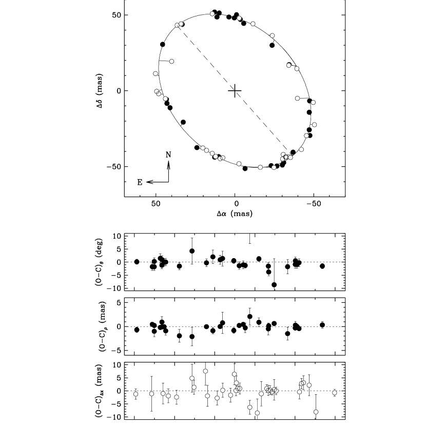
Figure 8.— Same as Fig. 6 and Fig. 7 for all long-baseline interferometric observations of Capella except those of Hummel et al. (1994). $O\!-\!C$ residuals are shown at the bottom, separately for observations made originally in polar coordinates ($\theta$, $\rho$ ; filled circles) and in rectangular coordinates ($\Delta x$, $\Delta y$ ; open circles). The scale of the position angle and separation residuals is the same as in Fig. 6 and Fig. 7, to facilitate the comparison.

Examination of Table Binary orbit, physical properties, and evolutionary state of Capella ($\alpha$ Aurigae) reveals that the residuals in $\theta$ for the observations by Merrill (1922) show a tendency toward negative values for the later dates. The earlier observations made by Anderson (1920) (and re-reduced by Merrill, 1922) show the opposite trend, with the exception of the very first measurement, which is of much lower quality and has a very large error. These trends were noticed already by Merrill, who offered as explanations either an instrumental effect or a real advance of the node. We find no evidence for a secular change in $\Omega$ in the other observations, so we tend to agree with McAlister (1981) that it is most likely an instrumental problem. As a test, we repeated the orbital solution solving for two position angle corrections in addition to the other 24 elements. We obtained $-0\fdg 5\pm 0\fdg 5$ for the earlier observations by Anderson, and $+1\fdg 4\pm 0\fdg 4$ for the later ones by Merrill, consistent with expectations. Adjusting the original values of $\theta$ for these offsets leads to a 1$\sigma$ decrease in the orbital period of Capella, and a slightly reduced uncertainty in $P$ of 17 sec. The change in all other elements and derived quantities is negligible.

Figure 9.— Motion of the photocenter of Capella relative to the center of mass of the binary (indicated by the plus sign) as seen by Hipparcos. See Fig. 7 for a comparison with the size of the relative orbit. The solid curve is the computed orbit from our global solution. Because these measurements are one-dimensional in nature, their exact location on the plane of the sky cannot be displayed graphically. The abscissa residuals are shown schematically with a filled circle at the predicted location, dotted lines representing the scanning direction of the satellite, and short perpendicular line segments indicating the undetermined location of the measurement on that line. The length of the dotted lines represents the magnitude of the $O\!-\!C$ residual from the computed location. Measurements with large residuals have been omitted for clarity. Motion is retrograde (clockwise).

Given that the components of Capella are slightly different, the size of the apparent orbit described by the center of light of the binary as seen in unresolved observations depends on the wavelength of the observation. Our inclusion of the Hipparcos data in the solution enables us to derive the brightness ratio $\ell_{\rm B}/\ell_{\rm A}$ between the stars in the passband of the satellite, denoted $H_{p}$. For this we make use of the fact that the semimajor axis of the photocenter and that of the relative orbit are related by $a^{\prime\prime}_{\rm phot}=a^{\prime\prime}(B-\beta)$, where $B=M_{\rm B}/(M_{\rm A}+M_{\rm B})$ is the fractional mass and $\beta=\ell_{\rm B}/(\ell_{\rm A}+\ell_{\rm B})$ is the fractional luminosity (see, e.g., van de Kamp, 1967). This leads to

$$(\ell_{\rm B}/\ell_{\rm A})_{H_{p}}=\left(\left[{K_{\rm A}\over K_{\rm A}+K_{\rm B}}-{a^{\prime\prime}_{\rm phot}\over a^{\prime\prime}}\right]^{-1}-1\right)^{-1}~{}.$$ (2)

Our resulting light ratio along with other estimates of the relative brightness are discussed in § 5. The projection of the photocentric orbit of Capella on the plane of the sky along with a schematic representation the Hipparcos measurements is seen in Figure 9. The much smaller size of the photocentric orbit compared to the relative orbit is illustrated in Figure 7.

5. The light ratio

The near equal brightness of the components of Capella has been a source of considerable confusion in the past. The quadrant of the ascending node and the time of nodal passage (or equivalently, the identity of the brighter star) have been changed more than once since the publication of the first set of astrometric orbital elements by Anderson (1920). The spectrophotometric study by Wright (1954), in which the author incorrectly concluded that the cooler star was the brighter one in the visible by $\sim$0.25 mag, played an important role in our understanding of the system for several decades, although unfortunately it also introduced biases in a number of other investigations that made use of that result. Examples include, among others, the interferometric study by Blazit et al. (1977a), who attempted the first angular diameter measurements of the stars, the Li abundance determinations by Wallerstein (1966) and Boesgaard (1971), and to some extent the ¹²C/¹³C ratio estimate by Tomkin et al. (1976), all of which adopted Wright’s brightness ratio. The history of this problem has been well summarized by Griffin & Griffin (1986), and further discussed by Barlow et al. (1993). Beginning in the early 1980s a number of authors used long-baseline interferometry and speckle interferometry techniques to unambiguously identify the hotter star as the brighter one in the visible (shortward of 7000 Å), and Griffin & Griffin (1986) provided a reasonable explanation for Wright’s spectroscopic result, which apparently referred to a difference between continuum heights rather than relative light intensities, and did not account for the difference in line blocking between the stars.

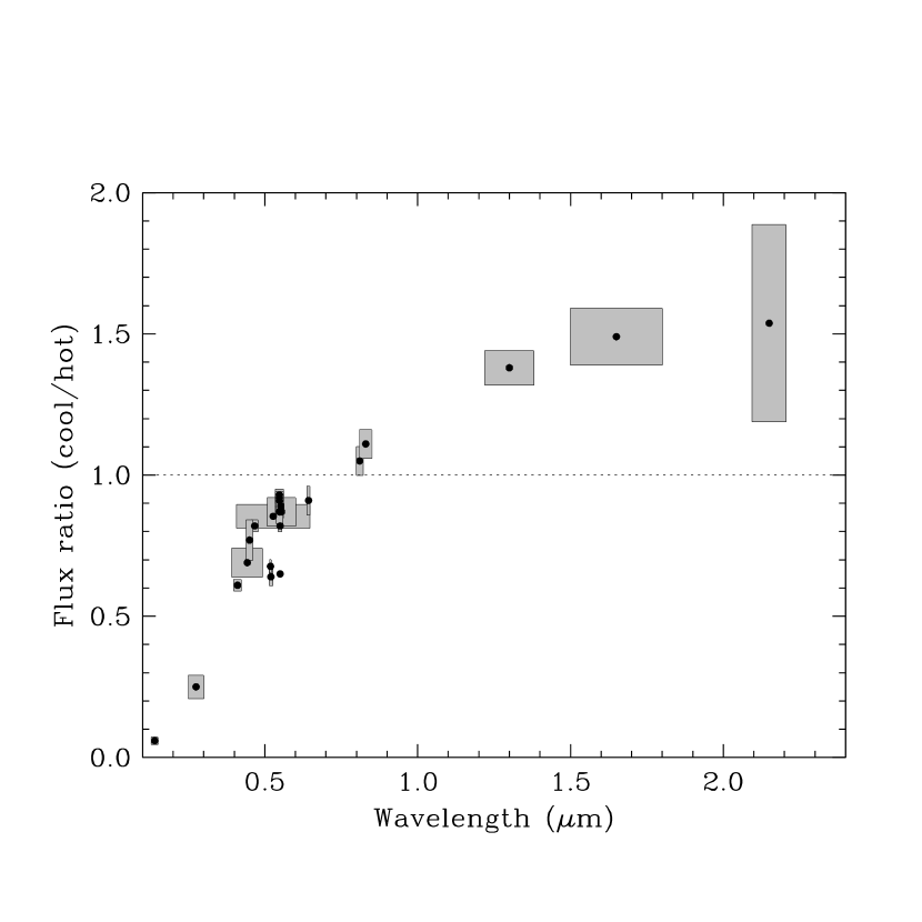
Figure 10.— Light ratio between the components of Capella as a function of wavelength. The shaded regions represent the uncertainty (vertical direction) and the FWHM of the passband (horizontal direction).

Nearly two dozen independent measurements of the relative brightness of the components are now available from the ultraviolet to the infrared. They are listed in Table 10, and are combined later with absolute photometry to derive effective temperatures for the components. Included also are our own light-ratio estimates from the CfA spectroscopy (see § 2.1) and from the Hipparcos observations (§ 4). The spectroscopic measurement reported by Strassmeier & Fekel (1990) refers to the ratio of continuum heights, rather than the intensity ratio. To convert to a true intensity ratio we have applied a correction for the line blocking based on appropriate synthetic spectra over the passband of their observations. We report the corrected value in Table 10. For uniformity the quantities listed in the table have all been converted to ratios $\ell_{\rm cool}/\ell_{\rm hot}$ ($=\ell_{\rm A}/\ell_{\rm B}$) between the cooler, slightly more massive star and the hotter star. A graphical representation of these measurements is seen in Figure 10. At wavelengths near the $V$ band the hotter star is slightly brighter, but around 7000 Å the ratio reverses, and the cooler, more massive star becomes dominant. This explains why some of the interferometric measurements such as those by Baldwin et al. (1996) and Kraus et al. (2005), which were made at red or near infrared wavelengths, have the quadrants reversed compared with measurements in the optical.

6. Angular diameters

The angular sizes of the components of Capella are large enough that they have been resolved by long-baseline interferometry on several occasions. They were first measured by Blazit et al. (1977a), who obtained uniform-disk angular diameters of $\Theta_{\rm UD}^{\rm A}=5.2\pm 1.0$ mas for the cooler primary star and $\Theta_{\rm UD}^{\rm B}=4.0\pm 2.0$ mas for the hotter star. However, these values assumed that the cooler star is brighter by 0.25 mag, following the results of Wright (1954), whereas we now know the cooler star is in fact the fainter one (see § 5). Unfortunately it is not possible to correct Blazit’s original estimates based on the information reported. Di Benedetto & Bonneau (1991) obtained a limb-darkened angular diameter of $\Theta_{\rm LD}^{\rm B}=6.28\pm 0.43$ mas for the secondary, along with a much more uncertain value of $\Theta_{\rm LD}^{\rm A}=9.6\pm 2.3$ mas for the primary, both measured in the $H$ and $K$ bands. Uniform-disk diameters in the $H$ band were published by Kraus et al. (2005) as $\Theta_{\rm UD}^{\rm A}=8.9\pm 0.6$ mas and $\Theta_{\rm UD}^{\rm B}=5.8\pm 0.8$ mas. The observations of Hummel et al. (1994) at wavelengths corresponding approximately to the $B$, $V$, and $I_{\rm C}$ bands gave limb-darkened angular diameters for Capella of $\Theta_{\rm LD}^{\rm A}=8.5\pm 0.1$ mas and $\Theta_{\rm LD}^{\rm B}=6.4\pm 0.3$ mas.

The above measurements are inhomogeneous due to the variety of limb-darkening corrections used. Those applied by Di Benedetto & Bonneau (1991) correspond to a scale factor of 1.035 between $\Theta_{\rm LD}$ and $\Theta_{\rm UD}$. Hummel et al. (1994) used limb-darkening coefficients from Manduca et al. (1977) and Manduca (1979), and Kraus et al. (2005) chose not to apply any corrections at all. To place all these measures on the same footing we have adopted limb-darkening coefficients from the tabulation by van Hamme (1993), and computed the $\Theta$ corrections following Hanbury Brown et al. (1974). The differences in these corrections compared to the original ones can be as large as 1.7%. The homogenized angular diameters are listed in Table 11. The resulting weighted averages are $\Theta_{\rm LD}^{\rm A}=8.47\pm 0.40$ mas and $\Theta_{\rm LD}^{\rm B}=6.24\pm 0.23$ mas. The uncertainties, which account for the scatter in the individual measurements, correspond to fractional errors of 4.7% for the primary and 3.7% for the secondary. These angular diameters, combined with the orbital parallax, yield the absolute radii of the components that are presented below.

As a check, independent estimates of the angular diameters may be obtained from the near-infrared surface-brightness relation of Di Benedetto (1998) for giant stars, which is very tight and has a scatter of only 1.4%. The required $V\!-\!K$ indices for the components of Capella are available from published photometry and are described in the next section (see also Table 13). After transformation of the photometry to the standard Johnson system following Carpenter (2001), we obtain $\Theta_{\rm LD}^{\rm A}=8.32\pm 0.75$ mas and $\Theta_{\rm LD}^{\rm B}=6.17\pm 0.65$ mas, in which the uncertainties include all photometric errors as well as the scatter of the calibration. While less precise, these values are in excellent agreement with the direct measurements from interferometry.

7. Chemical composition

Chemical composition plays a very important role in the comparison with models in the following sections, and provides important clues on the evolutionary state of the system. In this section we critically review and discuss all available abundance determinations in some detail, most of which have never been used before in the analysis of this binary.

Despite being such a bright star, the determination of the photospheric chemical composition of Capella has received relatively little attention by spectroscopists. The only detailed high-resolution study appears to be that of McWilliam (1990), in the context of a survey of 671 G and K giants. The value reported is [Fe/H] $=-0.37\pm 0.22$ on the scale of Grevesse (1984), in which the abundance of iron is $\log N({\rm Fe})=7.67$. This result is presumably based on the sharp lines of the primary. It does not seem that the study has accounted for the double-lined nature of the spectrum, which can influence the metallicity significantly in two ways. On the one hand, the continuum of the secondary (which has the same brightness as the other star at the wavelengths of the McWilliam (1990) spectra) will tend to fill in the lines of the primary at most phases, making them look weaker. On the other hand, the temperature adopted for Capella in this analysis (5270 K) was based on the combined-light photometry, and is too hot if assigned solely to the primary. This will generally result in abundances that are too high. It may compensate for the other effect to a certain degree, but the net bias is difficult to predict. Aside from the particular case of Capella, small systematic differences in the iron abundances between this work and others have occasionally been pointed out (e.g., Luck & Wepfer, 1995; Zhao et al., 2001; da Silva et al., 2006; Liu et al., 2007), and are probably traceable to systematic differences in the adopted surface gravities or microturbulent velocities.

Here we place the McWilliam (1990) [Fe/H] determination on the more recent scale of solar abundances by Grevesse & Sauval (1998), used in some of the models considered later, in which $\log N({\rm Fe})=7.50$. We obtain [Fe/H] $=-0.20\pm 0.22$, where the error is repeated from McWilliam (1990) and corresponds to the scatter of the individual iron line measurements rather than the uncertainty of the mean. The abundances of a dozen other elements studied by McWilliam (1990) were similarly converted to the same scale, and are collected in Table Binary orbit, physical properties, and evolutionary state of Capella ($\alpha$ Aurigae). For the purpose of comparison with the models in § 9.1, which assume solar-scaled abundances, we follow Valenti & Fischer (2005) and adopt the average of all elements as an overall indicator of metallicity: [m/H] $=-0.34\pm 0.07$. The uncertainty given here is the error of the mean. There is no evidence for enhancement of the $\alpha$ elements. All other indicators of the photospheric composition of Capella found in the literature are either circumstantial, contradictory, or inconclusive.

The photospheric ¹²C/¹³C isotope ratio has been measured in the optical for the primary star by Tomkin et al. (1976), who reported the value $27\pm 4$. As noted earlier, this study used the incorrect light ratio of Wright (1954) to subtract the contribution of the secondary to the observed continuum, although we do not believe this introduces a large error due to the differential nature of the measurement. This isotope ratio is a valuable indicator of evolution.

A large difference in the lithium abundance between Capella A and B was first pointed out by Wallerstein (1964), and confirmed by others. The hotter secondary has approximately two orders of magnitude stronger lithium than the primary. Measurements have been made by Wallerstein (1966), Boesgaard (1971), Pilachowski & Sowell (1992), Liu et al. (1993), and Randich et al. (1994), in which the first two are affected by the use of Wright’s light ratio, and the latter three adopted effective temperatures somewhat different from ours. The measurements by Pilachowski & Sowell (1992) appear to be the most reliable, although the others are generally consistent when adjusted for the modern light ratio. Here we have used the Pilachowski & Sowell (1992) equivalent width measurements for the Li I 6708 Å feature ($25\pm 2$ mÅ and $200\pm 10$ mÅ for the primary and secondary, respectively). We recalculated the abundances using the models by Pavlenko & Magazzù (1996), accounting for the temperature and gravity differences as well as non-LTE effects (not considered in the original analysis). We obtain revised lithium abundances of $\log N({\rm Li})=1.3\pm 0.2$ for the primary and $\log N({\rm Li})=3.2\pm 0.3$ for the secondary, in which the uncertainties include all measurement errors as well as possible errors in the microturbulent velocity following Pilachowski & Sowell (1992). To be conservative, the uncertainties have been further increased by 0.1 dex to account for slight extrapolations that were necessary in using the Pavlenko & Magazzù (1996) tables.

As an active binary system, Capella has been studied extensively in the ultraviolet and X rays for decades using virtually every space facility capable of observing at those wavelengths. It was in fact the first X-ray detection of a stellar corona other than the Sun, made by sounding rockets (Catura et al. 1975; see also Fisher & Meyerott 1964; Ayres et al. 1995). At ultraviolet wavelengths, Böhm-Vitense & Mena-Werth (1992) have presented evidence that reliable abundance ratios between carbon and nitrogen can be determined for giant stars from measurements of the emission fluxes of the C IV $\lambda$1550.8 and N V $\lambda$1238.8 lines in the lower transition layers between the stellar chromosphere and the corona, and that these ratios show good correspondence with the photospheric abundance ratios. Emission fluxes for these lines have been measured in Capella by a number of authors. However, early observations did not clearly resolve the contribution of the two components, of which the primary represents only $\sim$10%. This was first achieved by Linsky et al. (1995) based on high spectral resolution observations with HST. Using the fluxes they reported, we have derived the C/N ratios for Capella and use them below as diagnostics of evolution.

Abundance determinations for Capella have also been made by many authors from X-ray observations of coronal lines. With current instrumentation it is generally not possible to separate the spectral contribution of the two components in X rays, as it is in the UV. Ishibashi et al. (2006) and others have reported that the cool primary often dominates the coronal emission in this spectral region, although its flux is variable with time. Others find a more nearly equal contribution (e.g., Linsky et al., 1998). Therefore, any measurements may refer mainly to the primary, but are likely to be contaminated by the secondary. Most of these observations have revealed enhanced nitrogen (see, e.g., Mewe et al., 2001; Schmitt & Ness, 2002; Audard et al., 2003; Argiroffi et al., 2003). Mean abundances averaged over all other elements from these studies typically indicate a sub-solar composition, in qualitative agreement with the photospheric determinations of McWilliam (1990). However, coronal metallicity measurements are highly model-dependent (see, e.g., Brickhouse et al., 2001), and individual values sometimes show a large scatter from author to author. Furthermore, in the Sun’s coronal regions abundances are known to depend on the first ionization potential (FIP) of the element considered (e.g., Feldman & Widing, 2007). In view of these complications, we have preferred not to make use of these data here. Nevertheless, the nitrogen enhancement constitutes an interesting piece of chemical evidence for the evolved state of the primary, as recognized by many authors, since it is a natural consequence of the CNO cycle for stars that have already experienced first dredge-up (see below). Careful consideration of the FIP effect in Capella suggests there may be even closer agreement between the overall coronal abundance and the photospheric value, which we believe is worth noting given our concerns expressed earlier about the latter. We discuss these coronal measurements and their patterns in Appendix C. All other useful abundance determinations for Capella described above are gathered in Table Binary orbit, physical properties, and evolutionary state of Capella ($\alpha$ Aurigae).

8. Absolute dimensions

The astrometric-spectroscopic orbital solution in § 4 yields directly the absolute masses of the components. The relative uncertainties (0.7% and 0.5%) represent a factor of 3 improvement over those of Hummel et al. (1994), which is critical for the comparison with stellar evolution models. We also obtained the orbital parallax. The formal uncertainty in the corresponding distance of $13.042\pm 0.028$ pc is only 0.2%. The absolute radii of the components follow from the angular diameters and the distance, and are $R_{\rm A}=11.87\pm 0.56~{}R_{\sun}$ and $R_{\rm B}=8.75\pm 0.32~{}R_{\sun}$. Relative to the orbital separation, these values correspond to 0.075 and 0.055, respectively, so the binary is well detached.

Effective temperatures for the individual stars in Capella have been estimated here in three different ways. A first determination relies on our spectroscopy, and is described in § 2.1: $T_{\rm eff}^{\rm A}=4900\pm 100$ K and $T_{\rm eff}^{\rm B}=5710\pm 100$ K. A second method is that employed by Hummel et al. (1994), who made use of their angular diameter measurements along with the apparent magnitudes and bolometric corrections to infer values of $T_{\rm eff}^{\rm A}=4940\pm 50$ K and $T_{\rm eff}^{\rm B}=5700\pm 100$ K, nearly identical to ours. We have updated that calculation using the average angular diameters from § 6, together with apparent visual magnitudes for the components as described below, and bolometric corrections $BC_{V}$ from Flower (1996). The results are $T_{\rm eff}^{\rm A}=4970\pm 154$ K and $T_{\rm eff}^{\rm B}=5687\pm 130$ K, in which the uncertainties in $BC_{V}$ and in all other measured quantities are included. A third method to estimate individual temperatures relies exclusively on photometry (color indices), and has been applied by a number of authors over the years giving results generally consistent with the above estimates. We return to this technique below. To our knowledge there are no other fundamentally different $T_{\rm eff}$ estimates available, except for those one might infer indirectly from the spectral types assigned to the components. For example, Strassmeier & Fekel (1990) applied a spectrum synthesis technique and found a good match to the primary and secondary in the standard stars Pollux ($\beta$ Gem, K0 III) and $\alpha$ Sge (G1 III). These classifications are roughly consistent with our $T_{\rm eff}$ estimates.

The information on the absolute photometry for Capella and the light ratios discussed earlier is collected in Table 13. We use it here to derive photometric estimates of $T_{\rm eff}$ for each star. The light ratios in the table are weighted averages of all values near the $B$, $V$, $R$, $I$, $J$, $H$, and $K$ passbands, respectively, and the combined-light magnitudes are taken from the database of Mermilliod et al. (1997). $R$ and $I$ magnitudes were transformed to the Cousins system following Leggett (1992), and the near-infrared magnitudes were placed on the 2MASS system using the transformations of Carpenter (2001). Individual uncertainties are taken as published. Color indices formed from these values are listed in the second section of the table. These are not strictly independent, but they at least provide a sense of the consistency of the measurements in different systems and the scatter one can expect from the external calibrations applied in each case. Color/temperature calibrations for giant stars by Ramírez & Meléndez (2005) were used to derive temperatures for each component as well as for the combined light (third section of Table 13). The metallicity adopted is the value [m/H] $=-0.34\pm 0.07$ based on the measurements by McWilliam (1990), described in the previous section. The temperature uncertainties reported in the table account for all photometric errors, the uncertainty in the assumed [m/H], and also the scatter of each color/temperature relation. Weighted average temperatures computed from the seven indices are listed as well. The values for both Capella A and B are in good agreement with the other two determinations described previously.

The last line of Table 13 presents the weighted average of the three independent $T_{\rm eff}$ determinations for each star, based on the spectroscopy, the quantities {$\Theta_{\rm LD}$, $V$, $BC_{V}$}, and photometry, respectively. To be conservative, the uncertainty of the photometric values have been increased by adding 100 K in quadrature to the formal errors prior to taking the average, in order to account for possible systematics in the color/temperature calibrations. This follows the discussions of Ramírez & Meléndez (2005) and Casagrande et al. (2006) concerning our knowledge of the absolute effective temperature scale. The final temperatures are $4920\pm 70$ K and $5680\pm 70$ K for the primary and secondary, respectively.

The very different rotational velocities of the components was already evident to spectroscopic observers a century ago. The $v\sin i$ values have since been measured by many investigators, mostly by traditional spectroscopic means but also with other methods such as the differential speckle interferometry technique of Petrov et al. (1996). These estimates are collected in Table 14 along with our own. For the most part the more recent determinations agree fairly well, considering the difficulty of the measurements.

The physical parameters for both components of Capella are summarized in Table 15. The luminosities were derived here from the well determined absolute magnitudes and bolometric corrections from Flower (1996). The uncertainties in $BC_{V}$ were propagated from the error in $T_{\rm eff}$, and an additional conservative error of 0.05 mag was added in quadrature. If we instead compute the luminosities directly from the radii and temperatures, the values are considerably more uncertain ($L_{\rm A}=74.2\pm 8.2~{}L_{\sun}$, $L_{\rm B}=71.5\pm 6.1~{}L_{\sun}$), but are consistent with the adopted estimates. The primary (cooler) star is the more luminous bolometrically, but is the fainter one in the visible. Also included in the table are the projected rotational velocities ($v_{\rm sync}\sin i$) computed under the assumption that the stars have their spins synchronized with the orbital motion and that the spin axes are perpendicular to the orbital plane. We discuss these values in § 9.

9. Discussion

The key properties that determine the evolutionary state of the giants in Capella are the masses. Prior to this study the values most often adopted (e.g., Nobuyuki & Saio, 1999) were those of Hummel et al. (1994), $M_{\rm A}=2.69\pm 0.06~{}M_{\sun}$ and $M_{\rm B}=2.56\pm 0.04~{}M_{\sun}$, which rely on the velocity semi-amplitudes of Barlow et al. (1993). These masses are 9% and 5% larger, respectively, than those in the present work. As noted in § 2.2, our primary velocity semi-amplitude is not very different from other determinations, but our secondary value is considerably smaller, and this drives both masses down. An independent check on the accuracy of $K_{\rm B}$ can be made with the available astrometry (specifically, the Hipparcos observations), without using any secondary velocities. This is because the Hipparcos measurements are on an absolute frame of reference (ICRS) and therefore contain strong information on the trigonometric parallax, and the parallax is related to $K_{\rm B}$ via eq.(1). We carried out an orbital solution in which our secondary velocities were given zero weight, and the result for the secondary semi-amplitude is $K_{\rm B}=26.01\pm 0.62$ km s^-1. This is considerably more uncertain than the spectroscopic value of $26.260\pm 0.087$ km s^-1, but is still perfectly consistent with it, while at the same time being more than 2$\sigma$ away from the determination by Barlow et al. (1993). This suggests our masses for Capella are more accurate than previously determined, in addition to having smaller formal errors, and we proceed below to compare them along with other observations against theory.

9.1. Comparison with stellar evolution models

Detached binary systems such as Capella that are composed of two giant stars and show double-lined spectra are rare, and they provide important tests of models in a relatively short-lived phase of stellar evolution. Their component masses are necessarily very close to each other, and a precise measurement of the mass ratio $q$, as we provide here, becomes critical to establishing their state of evolution unambiguously.

The evolutionary status of Capella has been a subject of debate for decades. While there is general consensus that the hotter secondary is crossing the Hertzprung gap and approaching the base of the giant branch (RGB), opinions have varied on the precise location of the primary, in large part because of uncertainties in the masses as well as the effective temperatures and luminosities used to place the star on the H-R diagram. Capella is perhaps unique in that, in addition to those properties, a wealth of other information is available to aid in determining its evolutionary state, including the surface Li abundances of both stars, the ¹²C/¹³C isotope ratio for the primary, C/N ratios, and activity indicators in the optical, ultraviolet, and X rays. The progenitors of Capella were late B- or early A-type stars. When such stars leave the main sequence, they develop convective envelopes that deepen significantly as they approach the giant branch, mixing the outer layers with matter from the interior partially processed through the CNO cycle. As a result, fragile elements such as lithium are burned deeper in the star decreasing the surface abundance of that element, and others such as ¹³C and ¹⁴N that are created at the expense of ¹²C are brought to the surface during the “first dredge-up”. This causes a dramatic reduction in the ¹²C/¹³C ratio and in the C/N ratio, both of which are measurable. Thus, surface abundances contain potentially important information on the evolutionary state of evolved stars like Capella.

Iben (1965) pioneered this approach by relying on early estimates of the lithium abundance of both components (Wallerstein, 1964, 1966) to conclude, based on his models, that the primary is a core helium-burning star. Compared to an alternate location on the ascending giant branch, the “clump” phase also seems more likely because it is longer-lived. This lifetime argument seems to have weighed heavily in most of the other studies in which the measured masses, temperatures and luminosities have been compared against stellar evolution models, including the work of Barlow et al. (1993), Hummel et al. (1994), Schröder et al. (1997), and Iwamoto & Saio (1999). On the other hand, Boesgaard (1971) concluded based on her own Li measurements, which differed from those of Wallerstein, that the primary is not in such an advanced evolutionary state. Similarly, Bagnuolo & Hartkopf (1989) found evidence in the small luminosity difference between the stars that the primary is still at the beginning of the RGB. They also argued for a much smaller difference in mass than indicated by the measurements at the time, and indeed our present determinations bring the mass ratio much closer to unity than implied by the spectroscopy of Barlow et al. (1993). Ayres et al. (1983) also took the view that the primary is not yet burning helium in its core based on the high levels of chromospheric activity implied by their ultraviolet observations, although the opposite conclusion was reached by Ayres (1988).

The significantly improved parameters we have derived for Capella, particularly the masses which are three times more precise than those previously available, offer an opportunity to revisit the issue of its evolutionary status. Among the many publicly available stellar evolution models, we initially focused on those that allow some flexibility in setting parameters such as the composition or the age (for isochrones). However, not all of these models extend past the helium flash, which is necessary to explore the more advanced core helium-burning phase for the primary, and thus we are somewhat limited in our choices.

As a starting point, we compare the observations against the widely used set of stellar models by Girardi et al. (2000), based on physics that are now standard in most current models, including convective core overshooting. The mixing length parameter is fixed in these models at the value $\alpha_{\rm ML}=1.68$, overshooting is set to $\alpha_{\rm ov}=0.25$, and the chemical composition adopted for the Sun is $Z_{\sun}=0.019$. Diffusion is not considered, although its effect is completely negligible for Capella. Neither is mass loss due to winds, which appears to be rather low according to most estimates (Drake & Linsky, 1986; Katsova & Scherbakov, 1998; Getman & Livshits, 1999). For convenience we have chosen to compare the observations against isochrones (thereby imposing the constraint of coevality) computed using the web interface provided by the authors. In addition to $M$, $L$, and $T_{\rm eff}$, we consider also the absolute radii since they are determined independently from the temperatures and luminosities and are of comparable precision. We explored a fine grid of ages and chemical compositions, and used as a figure of merit the $\chi^{2}$ defined as

$$\chi^{2}=\sum_{i=1}^{2}\left[\left({\Delta M\over\sigma_{M}}\right)_{i}^{2}+\left({\Delta T_{\rm eff}\over\sigma_{T_{\rm eff}}}\right)_{i}^{2}+\left({\Delta L\over\sigma_{L}}\right)_{i}^{2}+\left({\Delta R\over\sigma_{R}}\right)_{i}^{2}\right]~{},$$

in which the $\Delta$ quantities represent the differences between the measurements and the models for each star ($i=1,2$). The best match to the observations is achieved for a metallicity $Z=0.008$ (corresponding to [Fe/H] = $-0.38$) and an age of $\tau=537$ Myr. All four measured quantities are reproduced to within 1.4 times their nominal uncertainties (see Table 16, case A), and the primary star is located on the ascending branch. A similarly good fit to an isochrone of the same age and composition can be found with the primary on the descending branch (Table 16, case B), with only a slightly larger difference with that star’s measured effective temperature (1.7$\sigma$). These two fits are shown in Figure 11. No satisfactory match is found with the primary in the core helium-burning phase, which has been favored by most previous investigators. Although the detailed surface abundances are not included in the published tables for these models, recent work by Bertelli et al. (2008) extending the same series of calculations does provide typical values for some elements. For a 2.5 $M_{\sun}$ star similar to the Capella primary and a metallicity of $Z=0.008$, the predicted ¹²C/¹³C after the first dredge-up is 19.0. This is lower than the estimate of $27\pm 4$ by Tomkin et al. (1976). On the other hand, the C/N ratios show much closer agreement with theory. The predicted value for the primary at the end of first dredge-up is 0.67, which is only slightly higher than the measured value of $0.57\pm 0.06$. For the secondary, which has not yet experienced first dredge-up and may therefore be expected to still have its initial main-sequence value of 3.27, the measured value is in fact very close: $3.30\pm 0.16$.

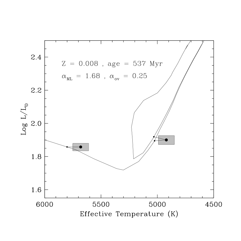
Figure 11.— Isochrone from the series by Girardi et al. (2000) for an age of $\tau=537$ Myr and $Z=0.008$ ([Fe/H] = $-0.38$) that provides the best match to the observations of Capella ($M$, $T_{\rm eff}$, $L$, and $R$ for both stars). Two different evolutionary states for the primary provide similarly good fits: one on the ascending branch, and the other on the descending branch prior to the beginning of of the core helium-burning phase. The large filled circles and shaded boxes correspond to the measured quantities for Capella and their uncertainties, while small dots on the isochrone correspond to the locations of the best fits. See Table 16.

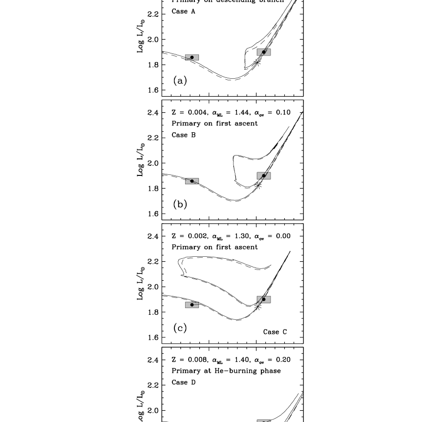
Figure 12.— Evolutionary tracks for Capella A (solid) and B (dashed) from the series of models by Claret (2004), for the exact masses determined here. The measured temperature and luminosity of each component are shown with the filled circles and error boxes. A thin line connects the measured positions with the best-fit location on each track. Four different scenarios are considered, focusing on the evolutionary status of the primary star. The parameters of each case and the location of the primary are as labeled. The asterisk on the primary tracks indicates the position where the models give a ¹²C/¹³C carbon isotope ratio exactly matching the measured value.

In order to provide more flexibility in exploring possible evolutionary stages for the primary, and also to gain better access to the detailed surface composition, we have considered a different set of models by Claret (2004) in which we can more easily vary not only the overall metallicity but also the mixing length and overshooting parameters. Evolutionary tracks were computed for the exact masses we measure. The best match is found for the same metallicity as before ($Z=0.008$, corresponding to [Fe/H] $=-0.33$ in these models, which adopt solar abundances from Grevesse & Sauval 1998) and convective parameters $\alpha_{\rm ML}=1.63$ and $\alpha_{\rm ov}=0.20$. As indicated in Figure 12a, the primary is on the descending branch, prior to the core helium-burning phase, and the age determined for the two components (553 Myr) is virtually identical to within 0.2%. Details of the differences in $T_{\rm eff}$, $L$, and $R$ for each star are given in Table 17 (case A), along with the goodness of fit ($\chi^{2}$). Lithium abundance calculations from these models are not up to date and have been found to give surface values that are much lower than other calculations. They are not considered further, although this has no impact on other calculations since Li is a low abundance element with no energetic importance. As in the previous models, the predicted ¹²C/¹³C isotope ratio for the primary is found to be lower than measured (19.18 versus $27\pm 4$, nearly a 2$\sigma$ difference). At face value the measured ratio seems inconsistent with any position for the primary of Capella other than on the first ascent. This is illustrated in Figure 13. The decrease in the isotope ratio shown in the top left panel is very rapid and follows closely the deepening of the convective envelope displayed on the lower left (first dredge-up). Values of ¹²C/¹³C are indicated on the evolutionary track in the right panel. The ratio changes from 85 to 20 in less than 1 Myr, so there is very little leeway to accommodate the measured value, which is predicted to occur in this model at a considerably lower luminosity and somewhat hotter temperature than observed, by 2.9$\sigma$ and 1.0$\sigma$, respectively (asterisk in Figure 13c). The alternative is an error in the measurement. We discuss this further below. On the other hand, the C/N ratios expected from these models are quite consistent with the observed values, as seen in Table 17.

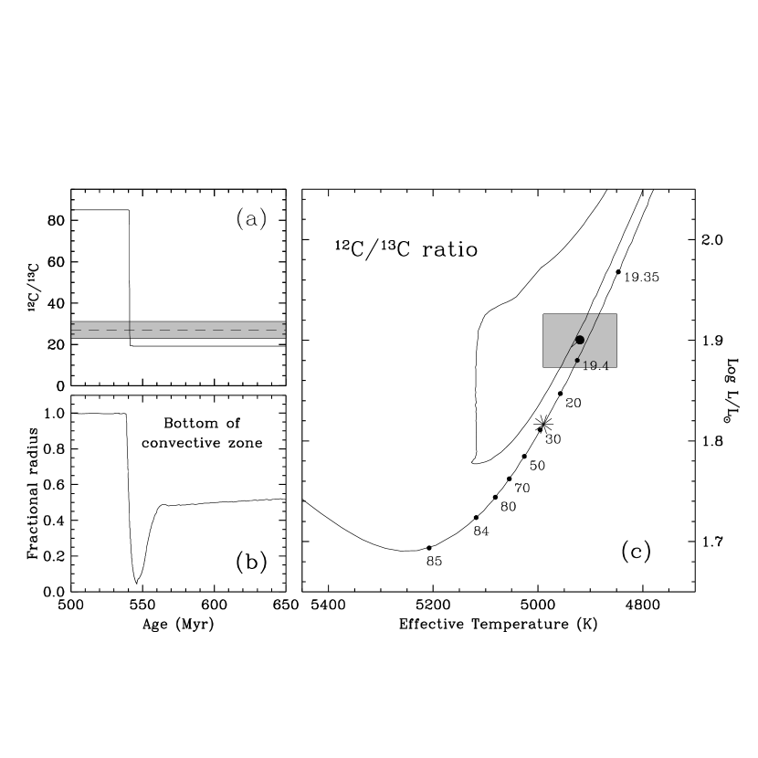
Figure 13.— Carbon isotope ratio evolution for the primary of Capella. (a) ¹²C/¹³C ratio as a function of age according to the Claret model in Figure 12a ($Z=0.008$, $\alpha_{\rm ML}=1.63$, $\alpha_{\rm ov}=0.20$; case A). The measurement is indicated with the dashed line, and the shaded area represents the 1$\sigma$ uncertainty. (b) Location of the bottom of the convective zone in terms of the radius of the star, showing the rapid deepening during the first dredge-up. (c) Close-up of the evolutionary track for the measured mass of Capella A from Fig. 12a showing the change in the carbon isotope ratio during the first ascent. The measured temperature and luminosity along with the error box are indicated. An asterisk marks the location on the track where the isotope ratio matches the measured value of $27\pm 4$.

Given the disagreement of the previous models with ¹²C/¹³C, we explored other possible matches that place the primary on the ascending branch, by varying both the mixing length and overshooting parameters. One such solution has $Z=0.004$ (corresponding to [Fe/H] $=-0.63$), $\alpha_{\rm ML}=1.44$, and a reduced overshooting of $\alpha_{\rm ov}=0.10$. The ages inferred for the two components agree to within 1.0%, and have a mean of 464 Myr (see Figure 12b). The carbon isotope ratio for the primary is underpredicted by about the same amount as before (Table 17, case B), and the location on the track that matches the measured ¹²C/¹³C value (asterisk) is only marginally closer to the measured luminosity and temperature of Capella A (2.7$\sigma$ and 0.8$\sigma$ discrepancies, respectively). A similar fit with the primary also on the ascending branch can be obtained with $\alpha_{\rm ML}=1.30$ and no overshooting ($\alpha_{\rm ov}=0.00$), but at an even lower metallicity of $Z=0.002$ that is probably unrealistic. The mean age in this case is 400 Myr, and the individual ages differ again by only 1.0% (Table 17, case C, and Figure 12c). The luminosity and temperature at which the primary model predicts a carbon ratio matching the observation are 2.0$\sigma$ and 0.9$\sigma$ away from the measured values, respectively. Setting aside the ¹²C/¹³C discrepancy for the moment, it is interesting to note that the measured C/N ratio for the primary appears to rule out all scenarios with that star on the ascending branch. While the predictions for (C/N)_B are still consistent with the observations, the expected (C/N)_A values are a factor of $\sim$3 too high (Table 17, cases B and C). Thus, the chemical evidence for Capella seems contradictory regarding the viability of the first ascent scenario.

We investigated also possible fits to the Claret models with the primary in the core helium-burning phase. While previous researchers have had no difficulty in finding satisfactory fits, in this case we are unable to achieve a match to $M$, $R$, $T_{\rm eff}$, and $L$ as good as in the scenarios discussed above. Evolutionary tracks with $Z=0.008$, $\alpha_{\rm ML}=1.40$, and $\alpha_{\rm ov}=0.20$ yield ages for the stars that differ by 16.4% (mean age of 589 Myr). The carbon isotope ratio for the primary is not reproduced (see Table 17, case D, and Figure 12d), but the C/N fractions are consistent with the measurements since the primary is well past the first dredge-up.

None of the stellar evolution models considered so far include the effects of rotation. Although the current rotation rates for Capella A and B are slow or moderate, this was not the case for the main-sequence progenitors, which were late B- or early A-type stars spinning at typical equatorial velocities of 150–200 km s^-1. Evolutionary tracks with rotation were computed for both components following Claret (1999) for the same set of parameters considered in case A above, under the assumption of rigid-body rotation. The initial angular rotation rate $\omega_{\rm rot}$ was set by requiring an approximate match between the predicted equatorial velocities at the current age and the measured values (de-projected from $v\sin i$ by assuming the spin axes are aligned with the orbital axis; see below). However, given that the rotation of the primary appears to be synchronized with the orbital motion (§ 9.2), one may expect tidal forces to have had some effect on that star whereas the secondary is farther from synchronization, and more likely to have evolved as an isolated star. Thus we only required a match to the rotation of the secondary, and we adopted the same value of $\omega_{\rm rot}$ for the primary on the grounds that the masses are the same within 1%, so all properties including rotation must have been very similar to begin with. The differences compared to non-rotating models are most obvious on the main sequence, where rotation renders the tracks some 500 K cooler, but are smaller toward the later evolutionary stages. We find that the best match between the rotating models and the observations is obtained for parameters nearly identical to those found earlier, at an age only 5 Myr older. The details of this comparison are included in Table 17, case E. The older age produced by these models compared to case A is reminiscent of the effect of overshooting, which extends the main-sequence lifetime. We also find that, although we did not require a match, the predicted rotational velocity of the primary reproduces the measured value exactly. This is an indication that the effects of tidal forces in damping the rotation of the star are relatively weak, given the long orbital period and relatively small relative radii of the components ($R_{\rm A}/a\approx 0.075$ and $R_{\rm B}/a\approx 0.055$, respectively). Another way of looking at this is to examine the evolution of the rotation rate for each star due solely to changes in the moment of inertia with time, under the assumption of rigid-body rotation and conservation of angular momentum without including tidal forces. These rotation rates relative to their initial values on the zero-age main sequence (ZAMS) are depicted in Figure 14 for both components as a function of time, for the models with $\alpha_{\rm ML}=1.63$. The inset shows the ratio of these two curves near the present age of the binary, which should correspond to the actual ratio of the rotational velocities if the stars started out with the same value on the ZAMS and if tidal forces are unimportant. There is in fact good agreement with the measured ratio of $v_{\rm B}\sin i/v_{\rm A}\sin i=7.1\pm 1.5$ (horizontal shaded area) at the evolutionary age determined with these models (vertical shaded area).

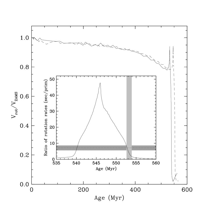
Figure 14.— Evolution of the rotation rates of Capella A (solid line) and B (dashed line) relative to their values on the ZAMS, according to Claret models with $Z=0.008$, $\alpha_{\rm ML}=1.63$, and $\alpha_{\rm ov}=0.20$ (case A). The inset shows the ratio of these curves (secondary divided by primary) along with the measured ratio of the projected rotational velocities ($v_{\rm B}\sin i/v_{\rm A}\sin i=7.1\pm 1.5$; shaded horizontal band). The theoretical ratio agrees with the measurement at the evolutionary age of the system (shaded vertical band spanning the primary and secondary ages from Table 17). This suggests tidal forces within the binary, which are not accounted for here, are weak.

The comparisons made above against the stellar evolution models by Girardi et al. (2000) and Claret (2004) do not constitute very strong tests of the predictive power of theory because a number of parameters have been adjusted to produce a good fit to the observations of Capella, namely, the overall composition, the mixing length, and overshooting. We note that in both models the metallicity that seems to be favored ($Z=0.008$) is actually in very good agreement with the spectroscopic value (§ 7) derived from the work of McWilliam (1990), despite our concerns about possible biases in those measurements. Even if we accepted the latter as accurate, and had imposed that value on the models thereby eliminating $Z$ as a free parameter, $\alpha_{\rm ML}$ and $\alpha_{\rm ov}$ are still adjustable quantities. This is unavoidable because of the phenomenological way in which convection and mixing are treated in these “standard” models.

We have thus considered a third set of models based on the TYCHO stellar evolution code (Young et al., 2001a; Young & Arnett, 2005) that implements somewhat different prescriptions for some of the physical processes. Predicted surface abundances are available for all the elements in the network, including lithium, and rotation has not been considered for the present work. The models calculated with the most recent version of this code, TYCHO 8, have a partial implementation of results from a new, non-local hydrodynamic description of convection presented in Arnett et al. (2009). The key results implemented in this version are the boundary conditions for convective zones. Convective stability is evaluated based on the Richardson number ($Ri=N^{2}/(\partial u/\partial r)^{2}$). This compares the potential energy in stratification as measured by the Brünt-Väisälä frequency $N$ versus the kinetic energy in shear (including turbulent velocities). Using the Richardson criterion results in larger convective zones since thermodynamically stable regions in mixing length theory can be hydrodynamically unstable. The complete velocity integration described in Arnett et al. (2009) has not yet been implemented for this work. Convective velocities are calculated according to mixing length theory with a mixing length equal to the depth of the convection zone, according to Arnett et al. (2009). This eliminates $\alpha_{\rm ML}$ as a free parameter. For very deep convective zones the simulations suggest there may be a saturation in the mixing length at a value of roughly 1.5–2.5 as dissipative processes become important. We place this saturation near the lower limit at 1.64. The models also include wave-generated mixing from intermittent turbulence and slow circulation according to Young & Arnett (2005). For most of the star’s history the convection is relatively shallow ($l_{\rm CZ}<2h_{p}$, where $l_{\rm CZ}$ is the depth of the convection zone and $h_{p}$ is the pressure scale height) except in the photosphere. In this regime the convective description has no free parameters. On the RGB, however, the convection zone has a very large density gradient over its depth. This has two effects. First, significant radiative losses from a fluid parcel can occur over a single convective traverse. Secondly, the sound speed drops with increasing radius and decreasing density. Initially strongly subsonic flows can generate shocks in the outer regions of the convective zone causing more dissipation. Unfortunately, we do not yet have a satisfactory quantitative theoretical description of this process, so we are forced to parametrize it. We introduce a geometric parameter $g_{\rm ML}$ (compare to the geometric parameter introduced by Böhm-Vitense (1958) for mixing length) which describes the aspect ratio of a convective fluid parcel. The value of the Böhm-Vitense parameter gives a surface-to-volume ratio less than that of a sphere. If we compare our parameter to the mixing length context, values of 1 to 1000 are a reasonable range to account for true geometric differences for large surface area turbulent flows, radiative losses over large temperature gradients, and hydrodynamic dissipative processes.

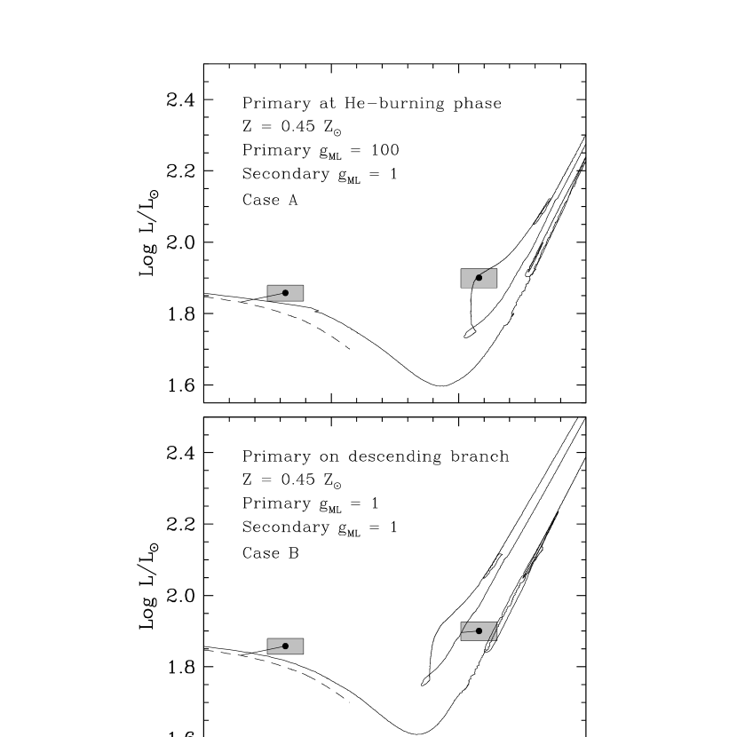
Figure 15.— Evolutionary tracks for the measured masses of Capella from the models of Young et al. (2001a) and Young & Arnett (2005). Two different scenarios are shown, focusing on the evolutionary state of the primary.

Using these models in the same way as before, the best match to the observations for Capella was found for evolutionary tracks with an overall metallicity of $Z=0.45Z_{\sun}$ (in which the solar composition is adopted from Asplund et al., 2005), corresponding approximately to [Fe/H] $=-0.35$. This is very similar to the composition that gave the best fits in the previous sets of models. For the secondary we used $g_{\rm ML}=1$ since it is only beginning to develop a deep convective envelope, and we are using a parametrization instead of a quantitative physical description. A modest increase may be supportable and provide a better fit. For the primary a value of $g_{\rm ML}=100$ provides a reasonable match to the global properties $M$, $R$, $T_{\rm eff}$, and $L$ with the star on the red clump (Table 18, case A), giving a mean age for the binary of $\sim$593 Myr and an age difference between the components of about 6%. A value for $g_{\rm ML}$ of 1 gives a good fit for the primary on the first descent of the RGB, but a poorer age match with the secondary (see Table 18, case B). An intermediate value of $g_{\rm ML}=10$ yields a less satisfactory agreement, also on the first descent. The above comparisons are shown graphically in Figure 15. The C/N abundance ratios predicted for the secondary in these two scenarios are quite consistent with the measured value, while those for the primary are more discrepant (see Table 18).

The ¹²C/¹³C ratios expected for the primary from the TYCHO models (19.0–19.6, depending on the evolutionary stage) are still significantly lower than the measured value of $27\pm 4$, as found before with the Claret models (18.9–19.2) as well as the Bertelli et al. (2008) models ($\sim$19.0). Other calculations indicate very similar values (e.g., Charbonnel, 1994). It would appear, therefore, that current theory systematically underestimates the carbon isotope ratio in this case, regardless of where the primary is located on the H-R diagram. Unfortunately there is only a single measurement of ¹²C/¹³C for Capella A, by Tomkin et al. (1976). A comparison of the results from that work for other stars that have also been measured by others seems to indicate some systematic differences, but it is difficult to tell which values are correct. For example, measurements by Tomkin et al. (1976) of the four Hyades giants $\gamma$ Tau, $\delta$ Tau, $\epsilon$ Tau, and $\theta^{1}$ Tau, which have masses only slightly smaller than Capella, give ¹²C/¹³C ratios of 19, 23, 22, and 20, respectively, while Gilroy (1989) reported 24, 26, 26, and 27, all systematically higher. It is possible that errors in the determination of the microturbulent velocity $\xi_{\rm t}$ can explain these differences, since Keller et al. (2001) and many others have shown that the ¹²C abundances are quite sensitive to $\xi_{\rm t}$ because the ¹²CN lines from which they are often measured are typically close to saturation. A cursory examination of measurements for other giant stars by different authors indicates similar discrepancies, which leads us to believe the uncertainties in some of these studies may be underestimated. A new measurement of the ¹²C/¹³C ratio for Capella A would be extremely helpful to settle this issue.

Table 18 shows that the surface lithium abundance predicted for the secondary of Capella from the TYCHO models is in agreement with the measurement, within the uncertainties, and is not much reduced from its main-sequence value. The primary lithium abundance, on the other hand, is larger than observed by about 3$\sigma$, regardless of the value of $g_{\rm ML}$. According to these models $\log N({\rm Li})$ is not expected to dip much below 1.9 even after the phase of core helium burning, as the star evolves up the asymptotic giant branch. Thus, it appears lithium burning in Capella A has been more efficient than predicted by theory during the first dredge-up, or there was additional burning afterwards. Unlike the case of ¹²C/¹³C, there are several independent measurements of the Li I $\lambda$6708 line for the primary, and they display rather good agreement. A possible explanation for the discrepancy is that in the current TYCHO models rotational and convective/wave sources of shear at the convective boundary are not correctly coupled. Mixing at the base of the envelope in the models will be less than that of the real star, and this could result in discrepancies in the abundances of low-temperature burning products.

As seen from the comparisons above with three different sets of evolutionary models, we are unable to find an evolutionary state for the binary that gives complete consistency with all absolute dimensions for both stars as well as all chemical indicators, simultaneously. Partial matches are possible, indicating either deficiencies in our understanding of stellar evolution, observational errors in some quantities, or both. Other evidence of the evolutionary status of Capella has occasionally been considered by some authors, including activity indicators in the UV and X rays. For example, based on similarities with other stars, Ayres et al. (1983) estimated that the primary may be responsible for as much as half of the total 0.1–0.4 keV soft X-ray coronal emission from the system, even though it only accounts for a small fraction of the far-UV emission characteristic of the chromospheric layers. A comparison with the generally weaker coronal X-ray levels of clump giants led them to conclude that Capella A is crossing the Hertzprung gap for the first time, and is yet to go through the first ascent. Although this significant level of X-ray emission was subsequently confirmed by others (e.g., Linsky et al., 1998; Young et al., 2001b), this picture seems inconsistent with some of the chemical indicators discussed above. Additionally, clump giants are known to display a wide range of coronal emission levels (see, e.g., Pizzolato et al., 2000), perhaps indicative of activity cycles analogous to that of the Sun. Virtually all UV and X-ray studies after the mid 1980s have implicitly assumed the primary of Capella is a core-helium burning star, on the grounds that it would be very unlikely to find both components of a binary in a very rapid state of evolution such as the Hertzprung gap or the first ascent, given that the secondary is already known to be a first crosser. This could only happen if the mass ratio were very near unity, and that did not appear to be the case until now. Ayres (1988) proposed the primary may be in the early stages of core-helium burning, while other giants that are even more active such as $\beta$ Cet and the Hyades stars $\gamma$ Tau and $\theta^{1}$ Tau were considered to be in a more advanced clump phase (“blue loop”). Qualitative assessments of the evolutionary state based on the overall activity level remain problematic, and are not easily testable against models.

We conclude this section by pointing out that the detached nature of Capella, and therefore its value for testing stellar evolution theory, is beyond doubt. The size predicted for the primary at the tip of the giant branch from any of the models considered above is less than 35 $R_{\sun}$, and would still fit comfortably inside its critical Roche surface ($\sim$60 $R_{\sun}$). Thus, even if the primary were already in the clump, mass transfer by Roche-lobe overflow would have been avoided.

9.2. Comparison with tidal theory

Capella is a particularly favorable case to study the rotational state of the components. In addition to the measures of $v\sin i$ and the radii, the rotational periods $P_{\rm rot}$ of both stars have been measured as well. Shcherbakov et al. (1990) found that the radial velocity of the chromospheric He I $\lambda$10830 absorption line follows the velocity of the photospheric lines of the primary, unambiguously identifying this activity feature with that star. The equivalent width of the line was also seen to vary with a period indistinguishable from the orbital period, which was interpreted as the rotational signature of the primary. Katsova & Scherbakov (1998) confirmed this with additional data, and measured a rotation period of 103.97 days. They were also able to detect a weaker component of the He I line associated with the secondary star. The radial velocity of this feature again varied in phase with the photospheric velocities for Capella B, but its equivalent width was seen to vary with a period of 8.25 days, representing the rotation of the secondary. Strassmeier et al. (2001) detected the rotational signature of both stars in their H$\alpha$ photometry, with periods of $106\pm 3$ days for the primary and $8.64\pm 0.09$ days for the secondary. These observations make it very likely that the primary’s rotation is effectively synchronized with the orbital motion, while the secondary is spinning more than 12 times more rapidly. For the purpose of this work we adopt a compromise value of $P_{\rm rot}=8.5\pm 0.2$ days for Capella B.

With these periods and the measured radii, the predicted rotational velocities projected along the line of sight are $3.92\pm 0.19$ km s^-1 and $35.4\pm 1.5$ km s^-1 for the primary and secondary, respectively, under the assumption that the spin axes are aligned with the orbital axis. These predictions may be compared directly against the measured $v\sin i$ values in Table 14. We note, however, that most of those determinations — including our own — have ignored the additional broadening that comes from macroturbulence. This can be significant for giants and in our case is particularly important for the primary, which is a slow rotator. The only two determinations of $v_{\rm A}\sin i$ in the table that have accounted for macroturbulence (Fekel et al., 1986; Strassmeier & Fekel, 1990) are both smaller than ours, and average 4 km s^-1. A giant star with the spectral type of Capella A is expected to have a macroturbulent velocity $\zeta_{\rm RT}$ between 5 and 6 km s^-1 (see, e.g., Gray, 1982), whereas the synthetic templates we used in § 2.1 to determine $v\sin i$ have $\zeta_{\rm RT}=1.5$ km s^-1. A correction for this difference following Fekel et al. (1997) and Massarotti et al. (2008) brings our $v\sin i$ value for the primary down from 6.5 km s^-1 to about 5.0 km s^-1. For the secondary this effect hardly matters, but a similar correction assuming $\zeta_{\rm RT}\approx 7$ km s^-1 leads to $v_{\rm B}\sin i=35.6$ km s^-1. These are the values we adopt in the following (Table 15). The agreement with the predicted velocities, which is well within the errors, can be considered as an indication that the absolute radii based on angular diameters are accurate.

The binary system of Capella resembles in many respects that of the 76-day period eclipsing system TZ For (Andersen et al., 1991), which is also composed of giants. Both have a circular orbit, and one component in synchronous rotation while the other is super-synchronous. This puzzling situation is of course explained by tidal forces, which increase exponentially as the more massive primaries evolve first and expand in size. The result is a sharp drop in their rotation rates, and the damping of the orbital eccentricity. We have computed the critical times of rotational synchronization and orbital circularization for Capella according to the turbulent dissipation and radiative damping mechanisms by Zahn (1992, and references therein), as well as the hydrodynamical mechanism of Tassoul & Tassoul (1997, and references therein). Note that we calculate actual times rather than timescales, since the latter would be completely meaningless for giant stars such as Capella that have altered their structure drastically since the ZAMS, changing from having radiative to convective envelopes. Thus we have integrated the differential equations for the changes in the orbital eccentricity and rotation rates along the evolutionary tracks following the prescriptions of Claret et al. (1995, 1997), to properly account for the stellar properties during the radiative and convective phases of evolution. The results obtained using the Claret non-rotating models for Capella A and B for $Z=0.008$, $\alpha_{\rm ML}=1.63$, and $\alpha_{\rm ov}=0.20$ (case A) are illustrated in Figure 16. In this diagram the radii are plotted as a function of age, and the times of synchronization and circularization are indicated along with the evolutionary age of the system ($\bar{\tau}=553.2$ Myr). For the primary the theory of Zahn (1992) gives $\tau_{\rm sync,A}=545.8$ Myr, and for the secondary $\tau_{\rm sync,B}=559.8$ Myr, both of which agree with the observation that the primary already appears to have its rotation synchronized with the orbital motion while the secondary is clearly asynchronous. According to these models the spin of each star becomes locked with the orbital motion when the components reach their maximum size at the tip of the giant branch (Figure 16, top). Circularization occurs somewhat later, at $\tau_{\rm circ}=563.6$ Myr. Strictly speaking, this is larger than the age of the binary and the prediction is thus formally inconsistent with the apparent circularity of the orbit, although perhaps not by much considering the approximations in tidal theory. Similar calculations for the mechanism of Tassoul & Tassoul (1997) are shown in the bottom panel of Figure 16, and indicate formal consistency with the observations for all three critical times.

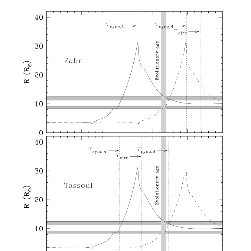
Figure 16.— Critical times of synchronization ($\tau_{\rm sync,A}$ and $\tau_{\rm sync,B}$) and circularization ($\tau_{\rm circ}$) for the components of Capella from tidal theory, shown in a diagram of radius versus age. Solid and dashed lines represent the predicted radii for the primary and secondary, respectively, according to Claret models with $Z=0.008$, $\alpha_{\rm ML}=1.63$, and $\alpha_{\rm ov}=0.20$ (case A). The measured radii are shown as horizontal shaded regions, and the evolutionary age of the system is indicated with a vertical shaded area. Calculations according to the tidal theory of Zahn (1992, and references therein) are shown at the top, and Tassoul & Tassoul (1997, and references therein) at the bottom.

We have repeated the calculations according to both tidal theories for the other scenarios considered earlier based on the Claret models, and the agreement with the observations varies. The results are summarized in Table 19. With one exception (case A and the mechanism of Tassoul & Tassoul, 1997), in no other scenario are all three critical times strictly consistent with reality, but the predictions are so close to the best-fit evolutionary ages that the results are very sensitive to the details of the models and the calculations. For example, the mere addition of rotation to the first set of evolutionary tracks examined above is enough to change the conclusions entirely regarding tidal theory, even though it hardly changes the stellar properties for the best fit. Thus, it is not possible to establish which tidal theory is more appropriate for Capella. We note, in this connection, that the theory of Tassoul has often been found to be too efficient, at least for main-sequence stars, giving critical times that are occasionally 1–2 orders of magnitude shorter than those by Zahn. In Capella that is not the case. Given that the critical times from these two theories tend toward each other in the limit of long periods, this again is an indication that tidal forces in this binary are relatively weak.

Another consequence of tidal forces in binaries is that the spin axes of the stars tend towards alignment with the orbital axis. Because the timescale for this is typically much shorter than for the other two effects, at least for main-sequence stars, it is almost universally assumed that the axes in binary systems are aligned. The simplifying advantage is that one can then set the inclination of the rotation axes equal to the orbital inclination, as we ourselves have done above, for example to infer equatorial rotational velocities. We note however, that this assumption may not always hold (see, e.g., the case of $\lambda$ Vir; Zhao et al., 2007). The timescale for alignment depends strongly on the ratio between the orbital and rotational angular momenta. This ratio is large for Capella because of the long orbital period, so the timescales for alignment are close to those for synchronization. As an example of such calculations, we use the rotating Claret models with $Z=0.008$, $\alpha_{\rm ML}=1.63$, and $\alpha_{\rm ov}=0.20$ (case E), and find that the alignment times according to Tassoul & Tassoul (1997) are 555.9 Myr for the primary and 563.6 Myr for the secondary. These are again so near the evolutionary age of 558 Myr for this scenario that it is difficult to draw general conclusions. At face value the primary is formally predicted to have reached alignment, while the secondary is still a few Myr from reaching it. The critical times for alignment according to Zahn (1992) are 562.3 Myr and 570.2 Myr, both of which are formally greater than the age, implying that the spin axes are not necessarily aligned. In Capella there is an observational constraint on this prediction, given by the rotation periods, $v\sin i$ values, and absolute radii determined for the two components. As indicated earlier in this section, there is very good agreement (particularly for the more discriminating secondary) between the measured $v\sin i$ values and the predicted rotational velocities, when the latter are projected along the line of sight using the well-known orbital inclination angle. This is evidence that the orbital axes are in fact closely aligned with the orbit, and we conclude that tidal theory does not clearly agree with the observations in this instance.

10. Concluding remarks

With our new spectroscopic observations of Capella and a global orbital solution that uses all available astrometric and radial-velocity measurements, the precision of the most important of the physical properties of the stars — their masses — has been improved threefold compared to previous values, and now stands at 0.7% for the primary and 0.5% for the secondary. These are at the level of the best available determinations from double-lined eclipsing binaries (see, e.g., Andersen, 1991). As others have pointed out, the mass ratio is perhaps more important in this case since it sets constraints on the differential evolution of the stars; that quantity is now known to even higher precision (0.36%). Based on the tests and crosschecks documented in this paper, it is our belief that the accuracy has also improved significantly. Our dynamical masses differ from earlier results by 9% and 5%, respectively, which has an enormous impact on the evolutionary state of giants such as these.

Our goal here has been to bring to bear all relevant information on the physical properties of Capella for a comprehensive discussion of the system in terms of its evolution. In addition to the masses, we report significantly improved determinations of the absolute radii, the effective temperatures, the luminosities, the rotational state of the stars, and the chemical composition, including the overall [m/H] index, the lithium abundance, and the ¹²C/¹³C and C/N ratios. We know of no other evolved system with so much high-quality information available. Sanity checks have been performed, whenever possible, to assess the accuracy of these quantities. Our expectation at the outset was then that we should be able to pinpoint the evolutionary state of these giants, particularly the primary, and validate current models of stellar evolution that seem to work so well on the main sequence. Instead, we find that there are now so many constraints that no single model is able to satisfy them all simultaneously, even when adjusting some of the free parameters in theory.

Three types of stellar evolution models have been considered, two based on standard convection prescriptions (Girardi et al., 2000; Claret, 2004) and one with an alternative formulation (TYCHO evolution code; Young et al., 2001a). We have also explored the role of rotation. In most cases it is possible to obtain reasonably good matches to $M$, $R$, $L$, and $T_{\rm eff}$ for both components at a variety of evolutionary states for the primary, of which the clump does not particularly provide one of the best matches. This is in contrast with most previous studies, which overwhelmingly place the primary in the core-helium burning phase, and is largely due to the fact that the mass ratio is now much closer to unity than previously believed (within 1%, versus 5% previously). This allows the “evolutionary gap” between the components to narrow considerably. These four properties alone are therefore insufficient to discriminate between different models or different states for Capella A.

Chemical constraints are seen to be particularly powerful in this case. We find that the overall metallicity [m/H] required for the models to match the properties of the two stars is in excellent agreement with the spectroscopic determination. However, the predicted ¹²C/¹³C values for the primary are systematically too low (at the $\sim$2$\sigma$ confidence level), if the measurement is to be taken at face value, and would require that component to be near the base of the RGB. This is inconsistent with the well-determined temperature and luminosity (or radius). Errors in the rather delicate measurement of the carbon isotope ratio cannot be ruled out, and a new determination would be highly beneficial. Similarly, models tend to overestimate the apparently well-measured lithium abundance of the primary (discrepancies at the $\sim$3$\sigma$ level), although they do match that of the secondary, which is essentially the initial value. The observed C/N ratios only permit the primary star to be on the descending branch prior to the helium-burning phase, or at the clump. Ascending branch scenarios are ruled out at the many-$\sigma$ level. A location on the descending branch would in fact be more likely than on the first ascent, given that the descent takes about 3 times longer (see footnote 9).

It may well be that the primary is indeed a clump giant, but the fact remains that current stellar evolution models fail to satisfy all of the observational constraints when considered jointly, for both components at the same time, and at a single age, whether the primary is in the core-helium burning phase or at any other location. Predictions are still very strongly dependent on the physics in the models, underscoring our incomplete understanding of many of these processes. The ¹²C/¹³C measurement suggests that convective mixing in the primary is less efficient than predicted, while the lithium determination appears to shows the opposite. It is also quite possible that the masses, as precise as they already are, need to be improved further by an order of magnitude given the sensitivity of the predictions. If that is the case, then both better spectroscopy and better astrometry will be required, since the latter contributes a non-negligible $\sim$0.3% to the present mass errors.

Tidal theory does not seem to fare much better. The circular orbit of Capella along with the evidence for synchronous rotation of the primary and asynchronous rotation of the secondary pose strong constraints that are in general not quite met by the mechanisms of Zahn (1992) and Tassoul & Tassoul (1997). Similarly with the alignment of the rotational axes with the orbital axis, which is observationally constrained by the measurements of $R$, $v\sin i$, and $P_{\rm rot}$. To be fair, however, the critical ages for circularization, synchronization, and alignment inferred from these models for the various scenarios considered are typically close to the evolutionary age in each case, so the results may be sensitive to the details of the calculations and are not conclusive.

Despite these challenges, much has been learned about Capella in its more than 100 years of observational history. It has been a favorite target of virtually every space facility and has provided, among many other results, very important insight into the structure and other properties of the coronae in active stars. Because it is so bright, nearby, and easy to observe, Capella remains a very important benchmark for testing our understanding of stellar physics in the advanced stages of evolution.

Appendix A The Greenwich visual observations of Capella

The relatively long orbital period of Capella from the spectroscopic studies of Newall (1899) and Campbell (1901) immediately suggested to investigators from the beginning of the 20th century the possibility that it might be detected as a visual binary, with a separation somewhat under 0$\farcs$1, according to the best estimates at the time. Foreseeing the potential of interferometry, Miller Barr (1900) suggested it should be resolvable with Michelson’s “interference apparatus” on a large telescope, although this would only come to happen two decades later. In the meantime, visual binary observers lost no time in attempting the measurement, even though predictions indicated the separation would be at or below the resolution limit of available telescopes. Aitken (1900) described five separate attempts with the Lick Observatory 36-inch Clark refractor (resolving power $\sim$0$\farcs$15), and on only one of those dates (1900 February 24) did he indicate that once or twice a slight elongation of the image was suspected, but that repeated measurements of the position angle showed a spread of some 60°, which he considered large enough to be a sign that no real elongation was observed. Hussey (1900, 1901) used the same telescope to look at Capella on multiple occasions, but also reported the images to be essentially round.

At about the same time, visual binary observers at the Greenwich Observatory took an interest as well, and reported seeing the image elongated with the 28-inch refractor (resolving power $\sim$0$\farcs$19) on 1900 April 4. They even recorded a position angle measurement for Capella. Over the next two years they continued observing the star regularly and making measurements of $\theta$, and on a few occasions they even ventured to estimate $\rho$. More than 100 position-angle measurements were made by 11 different observers, including the Astronomer Royal (Christie, 1900a, b, 1902, 1903). These observations have been viewed with suspicion ever since (e.g., Burnham, 1906). As pointed out by Ashbrook (1976), it is difficult to see how “a smaller instrument at sea level could consistently do what the 36-inch Clark refractor on Mount Hamilton found impossible”. No other visual observations elsewhere appear to have been successful; the only other recorded attempts, decades later by Wilson (1939, 1941), saw no elongation in Capella.

The most remarkable fact about the Greenwich observations, as discussed by Ashbrook (1976), is their overall agreement with the astrometric orbit of Merrill (1922), which was not published until twenty years later. Merrill himself had compared the Greenwich measurements with his orbit, but other than noting some relatively minor discrepancies, he made no judgement about them. Goos (1908) had also discussed these measurements in connection with his own spectroscopic observations, but this was also long before the astrometric orbit was known. Aside from these two studies, the Greenwich observations appear to have been largely ignored.

The refined orbital solution derived in the present work enables us to examine the accuracy of these measurements more closely. The circumstances of each observation were reconstructed based on published information. Most of the position angle estimates were made during the daytime, some at night, and a few during twilight, and all of them at hour angles greater than about 2$\text@frac{1}{2}$ hours (east or west) because of pointing limitations. A group of observations from 1900 April 23 to May 11 were considered by Christie (1900b) to be influenced by color effects, and we have not considered them here.

The first peculiar coincidence is that the observers correctly recorded the position angle of Capella to be decreasing with time (retrograde motion on the sky), which, as noted by Ashbrook (1976), they could not have known in 1900 since the only information available to them was that provided by the spectroscopic orbit. Secondly, the observations correctly placed the ascending node in the first quadrant as opposed to the third. Given the knowledge of the spectroscopic orbit, this can only be determined unambiguously from visual observations and if a difference in brightness is detected, which the Greenwich observers apparently saw, as reported by Christie (1900b). We now know that this difference is quite small in the visible, and as pointed out earlier, observers many decades later were still struggling with the difficulty of quadrant determination (see § 5). Furthermore, the actual position angle of the node implied by these observations is very roughly the correct value. The modern determination gives $\Omega=40\fdg 4$, and the estimate reported by Christie (1900b) after the first year of observation is $\Omega=80\arcdeg$. However, this value may be influenced by the fact that the Greenwich observers allowed the orbit to be eccentric, and in fact obtained a small but apparently significant value of $e=0.05$, whereas we now know the orbit is essentially circular (see § 4). Repeating the calculation for a circular orbit, and holding the period and epoch of nodal passage fixed at their known values, we obtain a revised estimate of $\Omega=57\arcdeg$ from the full sample of original Greenwich measurements, which is even closer to the modern value. Finally, the orbital inclination angle from this revised solution is $i=152\arcdeg$, also not far from the correct value of $137\fdg 2$.

In Figure 17a we show the position angle measurements as a function of time, compared with the prediction from our own orbital solution. They cover 7 full cycles of the binary. The second panel displays the $O\!-\!C$ residuals. A decreasing trend with time is clearly visible, although the magnitude of the residuals is quite modest considering the difficulty of the measurements, which can easily have errors of tens of degrees. The bottom panel (airmass versus time) shows that during the first few months the observers often made the measurements at large airmasses, whereas later on they observed closer to the zenith. It is also during those first few months that the residuals display the largest positive trend.

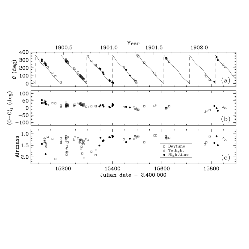
Figure 17.— Greenwich estimates of the position angle of Capella made from the elongated images. The different symbols indicate whether the observation was made during the daytime, twilight, or nighttime. (a) $\theta$ as a function of time, together with the computed orbit from the solution in this paper (which excludes these measurements); (b) $O\!-\!C$ residuals of the $\theta$ measurements from the computed orbit; (c) Airmass of each observation.

The agreements described above with the modern orbit of Capella are most intriguing. While it is certainly true that these measurements were made pushing the limits of what is possible for the visual technique, and that some of the most experienced observers of the time failed repeatedly to see any convincing elongation in the star’s image even using larger telescopes, the Greenwich observations are not easily dismissed. Ashbrook (1976) suspected that some of the measurements could have resulted — consciously or subconsciously — from foreknowledge of what the motion of Capella should be, based on the spectroscopic orbit that had just been published. The observers would certainly have known the average daily rate of change of the position angle, but nothing about variations in that rate throughout the orbit due to the inclination angle, or the direction of motion, and most certainly they could not have known in which quadrant the ascending node would be. It is quite likely, however, that since the period was known the measurements are not entirely independent, and some may well be wild guesses by inexperienced observers. We note, for example, that the quadrants of the individual observations as published are all consistent with the modern orbit, with the exception of two that need to be reversed. Rather than implying that the observers were able to determine the correct orientation in every case by detecting the slight difference in brightness, it seems more likely that they adjusted their $\theta$ values by $\pm$180° prior to publication, as needed for consistency with the initial measurements. This practice is still followed today, but indicates at the very least that the Greenwich observers were paying close attention to the agreement with the spectroscopic orbit. Three observers contributed almost 85% of all measures shown in Figure 17. About half of them were carried out by W. W. Bryant, and another third by W. Bowyer and T. Lewis. No systematic differences are seen among them. The very detailed observing notes they left indicate that they also made similar measurements of other very close binaries on some of the same nights on which they observed Capella, and to our knowledge those results have not been called into question.

After more than a century the Greenwich observations remain a mystery. H. F. Newall, who in his earlier spectroscopic study at that Observatory had discovered the binary nature of Capella and encouraged the visual observers to turn their attention to it (Newall, 1900), later expressed some doubts about those measurements in meetings of the Royal Astronomical Society, but believed that at least some were real (Newall, 1908). Bryant himself, the most active observer, took a similar view. In his own words (Bryant, 1907), “though many of the observations published are probably worthless, and may be ascribed to optical or psychological causes and to want of experience in judging of the suitability of observing conditions for what was practically a unique observation, yet there is little doubt that a certain proportion of the observations can be regarded as genuine.”

Appendix B Notes on the astrometric observations

We describe here the particulars of the astrometric measurements for Capella, including corrections to some of the original sources, or reasons that led us to reject some observations from the final solution.

Anderson (1920) and Merrill (1922): The six measurements reported by Anderson (1920) were re-reduced and are superseded in the paper by Merrill (1922). The P.A. for first of these six (on JD $2,\!422,\!323.65$) is admittedly very rough, and has been assigned an uncertainty of 10°, following the recommendation of the authors. The last of those 6 measurements (on JD $2,\!422,\!438.63$) was made during full daylight, and thus an angular separation was not reported because it was affected by the blue background that shifted the effective wavelength. The P.A. should be unaffected. The measurements reported in Table II by Merrill (1922) are nightly averages, but smearing should be insignificant given that the observing intervals were always less than 3 hours. The relative uncertainties used here for all these measurements account for the weights given by Merrill (1922), and are scaled as described in § 4. We note in passing that the dates of these observations have been translated into Bessellian epochs incorrectly in the orbital studies of McAlister (1981) and Barlow et al. (1993). The values used by those authors are exactly 0.5 days too small, possibly as a result of overlooking the fact that prior to 1925 astronomical time (GMT) was counted from noon, rather than midnight. The change in the P.A. and separation of Capella over half a day can be up to $2\fdg 4$ and 0.45 mas, respectively.

Kulagin (1970): The original position angle for the interferometric observation on 1968 February 18/19, listed as $303\fdg 5\pm 1\fdg 0$, is apparently incorrect (McAlister, 1981), and was changed by the latter author to $313\fdg 5\pm 1\fdg 0$ following a private communication from W. S. Finsen. Even after this change, the P.A. measurement gives a very large residual, and is excluded from our solution. Nothing wrong is seen with the separation measurement on this date.

Gezari et al. (1972): A speckle measurement of the angular separation is given with no epoch. It is compared in Table 1 of the original paper with predictions from the orbit by Merrill (1922) for JD $2,\!441,\!034.0$, which may then be taken as the date of observation. This date is likely to be rounded off, however, since the star was below the Palomar Observatory local horizon at the time. It corresponds to 1971 March 23, which also disagrees with indications in the text saying that “observations were made during twilight on 11 dates in 1971 April, June, and October”. A later paper by the same authors (Labeyrie et al., 1974, see below) does report measurements from the same site on 1971 March 23, so it seems likely they correspond to the same observations, although the angular separation reported is slightly different (possibly as a result of new reductions). We assume here that the latter measurements supersede the original one by Gezari et al. (1972).

Labeyrie et al. (1974): The dates for the ten speckle observations given here are only reported to 0.01 of a year, which is insufficient given that orbital motion is $\sim$10° and $\sim$2.1 mas over this time. Previous investigators (e.g., McAlister, 1981; Barlow et al., 1993) have used the dates at face value, not surprisingly with poor results. Furthermore, the first seven measurements were reported by Labeyrie et al. (1974) with precisely the same date (1971.23, presumably in Bessellian years), and were therefore simply averaged by subsequent investigators. It is clear from the text that the first four of these were taken on the night of 1971 March 23, probably during twilight at Palomar since the star was setting. We assign to these observations the date JD $2,\!441,\!034.67$. This is unlikely to be in error by more than 2 hours, which is good enough for our purposes. Inspection of measurements for other binaries from this source, as well as those of Capella, indicates that the position angles are systematically too small by several tens of degrees, a fact also noticed by others (despite the date problem). This may be due to a calibration error in these early speckle observations (McAlister, 1981), and we have chosen not to use those angles here. The remaining observations of Labeyrie et al. (1974) were likely taken a few nights later, but sufficiently precise dates are unavailable so we have excluded them.

Blazit et al. (1977a): The results of these interferometric measurements are taken from Figure 1. The date for the last one (1977.207) is given to one more significant digit in the text (1977.2066). Dates are assumed to be Bessellian years, more common in binary star publications, and also because the assumption of Julian years for the 1977.2066 measurement places the star below the horizon. All dates are converted to Julian days for use in the present work. The observation on 1977.125, which corresponds formally to JD $2,\!443,\!189.6$, is considered to have been made 0.1 days earlier, when the star was at a more plausible hour angle. This is well within the uncertainty in the original date (0.001 years), which corresponds to $\pm 0.36$ days. We note that the change in $\theta$ over 0.36 days is about 1$\fdg$6 on this date ($\rho$ only changes by 0.2 mas), so our date correction is not entirely insignificant. Uncertainties for the $\theta$ and $\rho$ measurements are estimated graphically from Figure 2 of this source.

McAlister (1977): The position angles of these speckle measurements were later slightly adjusted by the original author.

Weigelt (1978): Capella was unresolved in this speckle measurement made at an unspecified date with the 1.8m telescope at the Asiago Observatory (Italy).

McAlister & Hendry (1982a): The first of these speckle measurements, which were made at the resolution limit of the 2.1m telescope at Kitt Peak Observatory, gives large residuals both in $\rho$ and $\theta$, and was excluded from the solution.

Hege et al. (1983): The original speckle observations giving $\rho=0\farcs 042\pm 0\farcs 001$ and $\theta=331\arcdeg\ \pm 2\arcdeg$ (quadrant reversed for the present work) were reduced independently by Bagnuolo (1983a), who obtained $\rho=0\farcs 0420\pm 0\farcs 0015$ and $\theta=333\fdg 0\pm 1\fdg 2$. We have adopted here the average of these determinations, with the more conservative uncertainties. The date assigned to this observation (not precisely given by either author) is JD $2,\!444,\!637.6$, which corresponds to a reasonable hour angle at the Kitt Peak Observatory during twilight on UT 1981 February 2.

Koechlin et al. (1983): The first three interferometric measurements are apparently repeated from an earlier report by Koechlin et al. (1979), although they are slightly different in two cases. We consider them to supersede the original measurements. The date for the last of these three is also different from that given in the original, and is the one used here.

McAlister et al. (1987): These speckle measurements were later slightly corrected by the original authors.

McAlister et al. (1989): The speckle observation on JD $2,\!446,\!895.62$ (Bessellian epoch 1987.2717) gives very large residuals in both $\theta$ and $\rho$, and is excluded from our solution.

Isobe et al. (1990): Capella was unresolved in this speckle measurement made on 1988.8031 (Bessellian epoch) at the 2.12m telescope at the San Pedro Mártir Observatory (Mexico).

Hummel et al. (1994): Dates given in Table 2 of this source have been converted from Bessellian years to Julian dates for use in the present work. The interferometric visibilities on which the results are based have not been published, but were condensed into and published as $\theta$ and $\rho$ measurements for each night of observation (at 8^h UT).

Baldwin et al. (1996): The P.A. and separation values used in the present work were determined graphically from Figure 2 of this source, since they were not given explicitly. The epoch of observation for the first interferometric measurement is deduced from the calendar date mentioned in the text, along with the time during the night (2^h UT) from Figure 3. The second measurement is assumed to be taken at a similar time during the night of 1995 September 29.

Young & Dupree (2002): Exact times of observation for these direct-imaging HST measurements were not given in the original paper, but have been recovered from the HST online archives. The position angles are off by nearly 40° for unknown reasons, and have not been used here.

Kraus et al. (2005): The time of observation is taken to be the middle of the interval given for each measurement in Table 2 of this work.

Appendix C Coronal abundances in Capella

There is a significant body of literature on X-ray observations of Capella, which is not surprising given that it is the brightest steady coronal source in the X-ray sky. The available abundance determinations made from coronal emission-line fluxes have been collected in Table 20, and have been adjusted to conform to the standard solar abundances by Grevesse & Sauval (1998), for consistency with the photospheric determinations (see § 7). Coronal abundances in the Sun are known to depend on the first ionization potential (FIP), although the large-scale element fractionation processes presumably involved are not completely understood. Elements having low FIP ($<10$ eV) are overabundant compared to those with high FIP ($>10$ eV). We indicate the FIP values in Table 20, along with the average abundance for each element in the last column. The FIP trend has also been seen in some active stars, while others appear to show the opposite effect. For Capella there has been some debate about this issue, some authors claiming a mild FIP effect (Brickhouse et al., 2001; Audard et al., 2003; Argiroffi et al., 2003; Gu et al., 2006), or even an inverse effect (Bauer & Bregman, 1996), and others claiming no effect at all (Favata et al., 1997; Audard et al., 2001; Mewe et al., 2001). Some of this disagreement may stem from the use of different solar abundances, which is why we have homogenized all measurements here. As indicated in § 7, most authors agree that nitrogen is overabundant. The average abundance of the remaining high-FIP elements (C, O, Ar, Ne) is $-0.30\pm 0.04$, while that of the low-FIP elements (Ca, Ni, Mg, Fe, Si) is $+0.01\pm 0.03$, although it is likely that the true uncertainty is larger than indicated by these statistical errors. Sulfur has been excluded since its first ionization potential is close to the conventional dividing line of 10 eV. The FIP effect is thus clear in Capella: low-FIP elements are enhanced by a factor of $\sim$2 relative to high-FIP elements (see Figure 18). Furthermore, the evidence in the Sun indicates that high-FIP elements show better average agreement with the photospheric composition (Meyer, 1993; Feldman & Widing, 2007, and references therein). If the same were true in Capella, then the coronal abundance as measured from the high-FIP elements supports the photospheric determination of McWilliam (1990), which gives an overall metallicity of [m/H] $=-0.34\pm 0.07$. Under the same assumption, the enhancement of N relative to the high-FIP (or photospheric) composition would also be about a factor of 2, or slightly higher. Considering that this measure is diluted to some degree by the flux contribution from the (presumably normal composition) secondary, it appears to agree at least qualitatively with model predictions by Bertelli et al. (2008), which indicate a N enhancement of a factor of $\sim$3.1 for a post first dredge-up star. The average C/N ratio from Table 20 (note that since both C and N have high FIP, any residual FIP effect is more likely to cancel out) is approximately 0.52, though with a large uncertainty of at least 0.2–0.3 due to the scatter in C. An independent and perhaps more accurate estimate was reported by Schmitt & Ness (2002) as C/N $=0.91\pm 0.04$. The ratios predicted by the Bertelli et al. (2008) models are 0.67 after first dredge-up and 3.27 for the unevolved secondary, again roughly consistent with the measured values for the combined flux. Other models considered in § 9.1 give similar values.

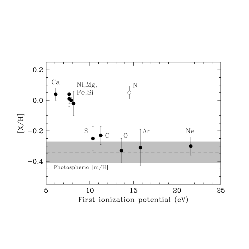
Figure 18.— Measurements of the coronal abundances in Capella from X-ray observations (combined flux of the two components) as a function of the first ionization potential of each element. The values shown are averages of several sources given in Table 20, and are taken from the last column of that table. Error bars represent the error of the mean, and all measurements are referred to the solar abundances as listed by Grevesse & Sauval (1998). Nitrogen is marked with a different symbol because it is expected to be enhanced due to convective mixing in the primary star occurring at the first dredge-up. The overall photospheric composition of Capella, [m/H] $=-0.34\pm 0.07$ (McWilliam, 1990), is indicated with the dashed line and gray error box, and refers to the same solar abundances.

Although a somewhat clearer and consistent picture than one might glean from a casual look at the literature seems to emerge from the above regarding coronal abundances in Capella, uncertainties are still rather large and our understanding of heating and element separation in the outer layers of stellar atmospheres is still limited.

Table 1CfA radial velocity measurements of Capella.

HJD		$RV_{\rm A}$	$RV_{\rm B}$	$\sigma_{\rm A}$	$\sigma_{\rm B}$	$(O\!-\!C)_{\rm A}$	$(O\!-\!C)_{\rm B}$
(2,400,000$+$)	Julian Year	(km s-1)	(km s-1)	(km s-1)	(km s-1)	(km s-1)	(km s-1)	Phase
46475.6179	1986.121	47.98	8.93	0.61	1.21	$-$0.42	$-$1.53	0.8781
46494.5383	1986.173	53.18	5.27	0.68	1.37	$-$0.65	$+$0.30	0.0600
50388.7228	1996.834	3.65	55.02	0.54	1.08	$-$0.01	$-$0.62	0.4963
50391.7233	1996.843	4.42	56.57	0.43	0.86	$+$0.45	$+$1.25	0.5251
50438.8498	1996.972	55.98	4.68	0.56	1.12	$+$0.57	$+$1.31	0.9781

Note. — Table 1 is presented in its entirety in the electronic edition of the Astrophysical Journal. A portion is shown here for guidance regarding its form and content.

Table 2Spectroscopic orbital solutions from published velocities for Capella.

	$\gamma$	Prim/Sec offset	$K_{\rm A}$	$K_{\rm B}$	$T$	$\sigma_{\rm A}$	$\sigma_{\rm B}$			Time span
Source	(km s-1)	(km s-1)	(km s-1)	(km s-1)	(HJD$-2,\!400,\!000$)	(km s-1)	(km s-1)	$N_{\rm A}$	$N_{\rm B}$	(days)
Campbell (1901)	+30.15 $\pm$ 0.14	$\cdots$	25.89 $\pm$ 0.18	$\cdots$	14865.54 $\pm$ 0.14	0.77	$\cdots$	31	$\cdots$	1486.0
Newall (1900)	+27.19 $\pm$ 0.55	$\cdots$	26.89 $\pm$ 0.83	$\cdots$	14969.34 $\pm$ 0.48	2.20	$\cdots$	23	$\cdots$	0121.0
Goos (1908)	+30.67 $\pm$ 0.27	0	25.83 $\pm$ 0.37	36.23 $\pm$ 1.45	17466.50 $\pm$ 0.25	1.56	5.41	35	19	1004.3
Sanford (1922)	+29.66 $\pm$ 0.08	0	27.06 $\pm$ 0.20	34.34 $\pm$ 1.49	23085.33 $\pm$ 0.14	0.27	3.36	7	4	0055.9
Struve (1939)	+31.44 $\pm$ 0.17	0	26.02 $\pm$ 0.24	31.09 $\pm$ 0.82	28180.59 $\pm$ 0.15	1.01	3.10	36	16	0753.7
Struve & Kilby (1953)	+29.30 $\pm$ 0.12	$\cdots$	26.46 $\pm$ 0.17	$\cdots$	31821.46 $\pm$ 0.12	0.83	$\cdots$	45	$\cdots$	8142.9
Wright (1954)	$\cdots$	$\cdots$	53.23 $\pm$ 0.63		34214.36 $\pm$ 0.50	2.42		19		0802.9
Batten & Erceg (1975)	+29.50 $\pm$ 0.15	$\cdots$	26.10 $\pm$ 0.20	$\cdots$	42119.27 $\pm$ 0.15	0.64	$\cdots$	18	$\cdots$	0274.0
Shen et al. (1985)	+29.57 $\pm$ 0.14	+0.84 $\pm$ 0.45	26.35 $\pm$ 0.19	29.75 $\pm$ 0.59	44927.73 $\pm$ 0.11	0.86	2.58	42	39	1534.8
Beavers & Eitter (1986)	+29.87 $\pm$ 0.13	0	26.14 $\pm$ 0.18	30.43 $\pm$ 0.50	45031.92 $\pm$ 0.12	1.33	3.85	105	91	1902.9
Shcherbakov et al. (1990)	+31.66 $\pm$ 0.59	$\cdots$	25.48 $\pm$ 0.83	$\cdots$	46593.65 $\pm$ 0.51	2.92	$\cdots$	29	$\cdots$	0957.6
Shcherbakov et al. (1990)	+28.79 $\pm$ 0.87	$\cdots$	23.0 $\pm$ 1.1	$\cdots$	46594.46 $\pm$ 0.86	3.62	$\cdots$	24	$\cdots$	0957.6
Batten et al. (1991)	+30.50 $\pm$ 0.12	0	26.29 $\pm$ 0.17	27.06 $\pm$ 0.46	42119.37 $\pm$ 0.11	0.46	1.31	15	15	0211.7
Barlow et al. (1993)	+29.14 $\pm$ 0.10	0	25.96 $\pm$ 0.11	27.70 $\pm$ 0.41	44615.96 $\pm$ 0.12	0.47	1.38	23	14	4532.6
Katsova & Scherbakov (1998)	+30.36 $\pm$ 0.47	$-$6.44 $\pm$ 0.95	22.43 $\pm$ 0.61	35.83 $\pm$ 1.21	48568.57 $\pm$ 0.34	2.77	2.64	40	16	1562.5
CfA observations (this work)	+29.66 $\pm$ 0.04	+0.27 $\pm$ 0.08	25.96 $\pm$ 0.04	26.27 $\pm$ 0.09	50857.21 $\pm$ 0.03	0.46	0.91	162	162	5037.2

Note. — The following radial-velocity measurements were rejected in computing these solutions: JD $2,\!445,\!002.6506$ (Shen et al., 1985, primary); $2,\!444,\!930.825$, $2,\!445,\!366.634$ (Beavers & Eitter, 1986, primary); $2,\!445,\!315.781$, $2,\!445,\!315.793$, $2,\!445,\!320.718$ (Beavers & Eitter, 1986, secondary); $2,\!446,\!345.71$ (Shcherbakov et al., 1990, primary from He I $\lambda$10830 measurements); $2,\!449,\!242.545$, $2,\!449,\!315.281$, $2,\!449,\!316.458$, $2,\!449,\!316.480$ (Katsova & Scherbakov, 1998, primary); and $2,\!449,\!443.384$ (Katsova & Scherbakov, 1998, secondary).

Table 3Historical radial velocity measurements of the primary component of Capella.

JD		$RV_{\rm A}$	$\sigma_{\rm A}$	$(O\!-\!C)_{\rm A}$
(2,400,000$+$)	Julian Year	(km s-1)	(km s-1)	(km s-1)	Phase	Source
13804.0360	1896.671	36.50	0.75	$-$0.72	0.7939	1
13820.0050	1896.715	53.90	0.75	$-$0.84	0.9474	1
13837.0030	1896.761	50.40	0.75	$+$0.31	0.1108	1
13839.0290	1896.767	47.00	0.75	$-$0.90	0.1303	1
13876.8650	1896.870	4.30	0.75	$+$0.15	0.4940	1

Note. — Table Binary orbit, physical properties, and evolutionary state of Capella ($\alpha$ Aurigae) is presented in its entirety in the electronic edition of the Astrophysical Journal. A portion is shown here for guidance regarding its form and content.

References. — (1) Campbell (1901); (2) Newall (1900); (3) Goos (1908); (4) Struve (1939); (5) Struve & Kilby (1953); (6) Beavers & Eitter (1986); (7) Shcherbakov et al. (1990); (8) Batten et al. (1991); (9) Barlow et al. (1993).

Table 4Interferometric measurements of Capella published in polar coordinates.

JD		$\theta$	$\rho$	$\sigma_{\theta}$	$\sigma_{\rho}$	$(O\!-\!C)_{\theta}$	$(O\!-\!C)_{\rho}$
(2,400,000$+$)	Julian Year	(°)	(mas)	(°)	(mas)	(°)	(mas)	Phase	Source
22323.65	1919.996	148.0	42.8	10.00	0.54	$-$8.66	$+$1.16	0.696	1
22368.63	1920.119	005.0	46.9	01.73	0.80	$+$1.46	$-$0.35	0.129	1
22369.65	1920.122	001.0	46.2	01.44	0.67	$+$0.94	$-$0.16	0.138	1
22370.66	1920.125	356.4	45.4	01.44	0.67	$-$0.08	$-$0.09	0.148	1
22399.63	1920.204	242.0	51.7	01.73	0.80	$+$0.91	$+$0.00	0.427	1

Note. — Table Binary orbit, physical properties, and evolutionary state of Capella ($\alpha$ Aurigae) is presented in its entirety in the electronic edition of the Astrophysical Journal. A portion is shown here for guidance regarding its form and content.

References. — (1) Merrill (1922); (2) Kulagin (1970); (3) Blazit et al. (1977a); (4) Hummel et al. (1994)

Table 5Interferometric measurements of Capella published in Cartesian coordinates.

JD		$\Delta x$	$\Delta y$	$\sigma_{\Delta x}$	$\sigma_{\Delta y}$	$(O\!-\!C)_{\Delta x}$	$(O\!-\!C)_{\Delta y}$
(2,400,000$+$)	Julian Year	(mas)	(mas)	(mas)	(mas)	(mas)	(mas)	Phase	Source
43773.6980	1978.723	$+$40.0	+19.4	6.70	0.76	$-$8.07	$-$0.49	0.904	1
43792.6460	1978.775	$+$14.3	+50.8	6.70	1.26	$-$1.09	$+$0.21	0.086	1
43798.6290	1978.792	0$-$2.8	+47.9	4.02	1.26	$-$1.00	$+$0.17	0.143	1
43805.6100	1978.811	$-$23.8	+36.4	2.68	0.51	$-$2.39	$-$0.28	0.210	1
43813.5880	1978.832	$-$34.2	+16.8	5.36	1.26	$+$4.85	$+$0.48	0.287	1

Note. — Table Binary orbit, physical properties, and evolutionary state of Capella ($\alpha$ Aurigae) is presented in its entirety in the electronic edition of the Astrophysical Journal. A portion is shown here for guidance regarding its form and content.

References. — (1) Koechlin et al. (1979); (2) Koechlin et al. (1983); (3) Baldwin et al. (1996); (4) Kraus et al. (2005).

Table 6Speckle and imaging measurements of Capella.

JD		$\theta$	$\rho$	$\sigma_{\theta}$	$\sigma_{\rho}$	$(O\!-\!C)_{\theta}$	$(O\!-\!C)_{\rho}$
(2,400,000$+$)	Julian Year	(°)	(mas)	(°)	(mas)	(°)	(mas)	Phase	Source
41034.6700	1971.224	$\cdots$	53.00	$\cdots$	1.36	$\cdots$	$-$0.85	0.572	1
41034.6700	1971.224	$\cdots$	54.00	$\cdots$	1.36	$\cdots$	$+$0.15	0.572	1
41034.6700	1971.224	$\cdots$	55.00	$\cdots$	1.36	$\cdots$	$+$1.15	0.572	1
41034.6700	1971.224	$\cdots$	56.00	$\cdots$	1.36	$\cdots$	$+$2.15	0.572	1
42643.1500	1975.628	35.00	53.00	5.76	3.40	$+$3.75	$-$2.78	0.035	1

Note. — Table Binary orbit, physical properties, and evolutionary state of Capella ($\alpha$ Aurigae) is presented in its entirety in the electronic edition of the Astrophysical Journal. A portion is shown here for guidance regarding its form and content.

References. — (1) Labeyrie et al. (1974); (2) Blazit et al. (1977b); (3) McAlister (1977); (4) McAlister (1978); (5) McAlister & DeGioia (1979); (6) Balega & Tiknonov (1977); (7) McAlister & Fekel (1980); (8) Morgan et al. (1980); (9) McAlister & Hendry (1982a); (10) McAlister & Hendry (1982b); (11) McAlister et al. (1983); (12) Dudinov et al. (1982); (13) Hege et al. (1983) and Bagnuolo (1983a); (14) Balega et al. (1984); (15) McAlister et al. (1987); (16) Balega & Balega (1985); (17) Hartkopf et al. (2000); (18) Balega & Balega (1987); (19) Bonneau et al. (1986); (20) McAlister et al. (1989); (21) McAlister et al. (1993); (22) McAlister et al. (1990); (23) Hartkopf et al. (1992); (24) Horch et al. (1999); (25) Young & Dupree (2002) (direct imaging rather than speckle); (26) Scardia et al. (2000); (27) Balega et al. (2004).

Table 7Hipparcos measurements of Capella and corresponding $O\!-\!C$ residuals.

HJD		$\Delta v$	$\sigma_{\Delta v}$	$O\!-\!C$
(2,400,000$+$)	Julian Year	(mas)	(mas)	(mas)	Phase
47921.1897	1990.079	$-$6.53	3.54	$-$7.11	0.7749
47921.2922	1990.079	$-$0.61	2.57	$-$1.19	0.7759
47933.1656	1990.111	$-$2.90	1.85	$-$0.99	0.8901
47933.2030	1990.111	$-$1.76	3.50	$+$0.16	0.8904
47965.5793	1990.200	$-$0.71	1.68	$+$0.87	0.2017

Note. — Table 7 is presented in its entirety in the electronic edition of the Astrophysical Journal. A portion is shown here for guidance regarding its form and content.

Table 8Summary of data sets used in the orbital solution for Capella, along with typical uncertainties.

Source	Measurements	$\sigma$
Spectroscopic observations
Campbell (1901)	31 measures of $RV_{\rm A}$	0.74
Newall (1900)	23 measures of $RV_{\rm A}$	2.12
Goos (1908)	35 measures of $RV_{\rm A}$	1.52
Struve (1939)	36 measures of $RV_{\rm A}$	0.97
Struve & Kilby (1953)	45 measures of $RV_{\rm A}$	0.91
Beavers & Eitter (1986)	105 measures of $RV_{\rm A}$	1.27
Shcherbakov et al. (1990)	29 measures of $RV_{\rm A}$	3.14
Batten et al. (1991)	15 measures of $RV_{\rm A}$	0.48
Barlow et al. (1993)	23 measures of $RV_{\rm A}$	0.45
CfA (this paper)	162 measures of $RV_{\rm A}$ and $RV_{\rm B}$	0.44 , 0.89
Astrometric observations
Merrill (1922)	16 measures of $\theta$ and 15 of $\rho$	1.50 , 0.62
Kulagin (1970)	11 measures of $\theta$ and 12 of $\rho$	1.10 , 1.52
Blazit et al. (1977a)	3 measures of $\theta$ and $\rho$	5.98 , 3.39
Koechlin et al. (1979, 1983)	25 measures of $\Delta x$ and $\Delta y$	2.67 , 0.67
Hummel et al. (1994)	40 measures of $\theta$ and $\rho$	0.13 , 0.11
Baldwin et al. (1996)	2 measures of $\Delta x$ and $\Delta y$	0.93 , 1.57
Hipparcos (Perryman et al., 1997)	41 measures of $\Delta v$	2.82
Young & Dupree (2002)	4 measures of $\rho$	2.19
Kraus et al. (2005)	5 measures of $\Delta x$ and $\Delta y$	0.26 , 0.19
Speckle observers	47 measures of $\theta$ and 53 of $\rho$	1.18 , 1.19

Table 9Orbital solution for Capella.

Parameter	Value
Adjusted quantities
$P$ (days)	104.02173 $\pm$ 0.0002200
$a^{\prime\prime}$ (mas)	56.408 $\pm$ 0.0250
$i$ (deg)	137.212 $\pm$ 0.05100
$\Omega_{\rm J2000}$ (deg)	40.421 $\pm$ 0.0640
$T$ (HJD$-$2,400,000)	47528.514 $\pm$ 0.016string
$\gamma$ (km s-1)	$+29.653$ $\pm$ 0.0350+
$K_{\rm A}$ (km s-1)	26.005 $\pm$ 0.0360
$K_{\rm B}$ (km s-1)	26.260 $\pm$ 0.0870
$a^{\prime\prime}_{\rm phot}$ (mas)	2.08 $\pm$ 0.69
$\Delta\alpha^{*}$ (mas)	$-$0.26 $\pm$ 0.80+
$\Delta\delta$ (mas)	$-$0.30 $\pm$ 0.57+
$\Delta\mu_{\alpha}^{*}$ (mas yr-1)	$+$0.32 $\pm$ 0.99+
$\Delta\mu_{\delta}$ (mas yr-1)	$-$0.08 $\pm$ 0.59+
$f_{\rho}$	1.0400 $\pm$ 0.0035
$\Delta_{\rm AB}$ (km s-1)	$+$0.267 $\pm$ 0.079+
$\Delta_{1}$ $\langle$CfA $-$ Campbell (1901)$\rangle$ (km s-1)	$-$0.48 $\pm$ 0.14+
$\Delta_{2}$ $\langle$CfA $-$ Newall (1900)$\rangle$ (km s-1)	$+$2.12 $\pm$ 0.45+
$\Delta_{3}$ $\langle$CfA $-$ Goos (1908)$\rangle$ (km s-1)	$-$0.93 $\pm$ 0.26+
$\Delta_{4}$ $\langle$CfA $-$ Struve (1939)$\rangle$ (km s-1)	$-$1.82 $\pm$ 0.17+
$\Delta_{5}$ $\langle$CfA $-$ Struve & Kilby (1953)$\rangle$ (km s-1)	$+$0.34 $\pm$ 0.14+
$\Delta_{6}$ $\langle$CfA $-$ Beavers & Eitter (1986)$\rangle$ (km s-1)	$-$0.37 $\pm$ 0.13+
$\Delta_{7}$ $\langle$CfA $-$ Shcherbakov et al. (1990)$\rangle$ (km s-1)	$-$2.37 $\pm$ 0.59+
$\Delta_{8}$ $\langle$CfA $-$ Batten et al. (1991)$\rangle$ (km s-1)	$-$0.90 $\pm$ 0.13+
$\Delta_{9}$ $\langle$CfA $-$ Barlow et al. (1993)$\rangle$ (km s-1)	$+$0.50 $\pm$ 0.10+
Derived quantities
$M_{\rm A}$ ($M_{\sun}$)	2.466 $\pm$ 0.018
$M_{\rm B}$ ($M_{\sun}$)	2.443 $\pm$ 0.013
$q\equiv M_{\rm B}/M_{\rm A}$	0.9903 $\pm$ 0.0036
$a$ ($10^{6}$ km)	110.06 $\pm$ 0.2300
$a$ (AU)	0.7357 $\pm$ 0.0015
$\pi_{\rm orb}$ (mas)	76.67 $\pm$ 0.170
Distance (pc)	13.042 $\pm$ 0.0280
$\mu_{\alpha}^{*}$ (mas yr-1)	$+$75.84 $\pm$ 0.990+
$\mu_{\delta}$ (mas yr-1)	$-$427.21 $\pm$ 0.5900+
$(\ell_{\rm B}/\ell_{\rm A})_{H_{p}}$	1.171 $\pm$ 0.057

Table 10Relative brightness measurements for Capella.

	Wavelength	Bandwidth
Source	($\mu$m)	($\mu$m)	$\ell_{\rm cool}/\ell_{\rm hot}$
Young & Dupree (2002)	0.1400	0.0200	0.059 $\pm$ 0.012
Young & Dupree (2002)	0.2750	0.0500	0.25 $\pm$ 0.04
Bagnuolo & Sowell (1988)	0.4108	0.0223	0.61 $\pm$ 0.02
Griffin & Griffin (1986)	0.4425	0.0988	string0.69 $\pm$ 0.05
Hummel et al. (1994)	0.4500	0.0200	0.77 $\pm$ 0.07
Bagnuolo & Sowell (1988)	0.4669	0.0202	0.82 $\pm$ 0.02
CfA spectroscopy (this paper)	0.5188	0.0045	0.677 $\pm$ 0.023
Hege et al. (1983)	0.5200	0.0100	0.64 $\pm$ 0.03
Hipparcos (this paper)	0.5275	0.2378	0.854 $\pm$ 0.041
Bagnuolo & Sowell (1988)	0.5478	0.0253	0.93 $\pm$ 0.02
Bagnuolo & Sowell (1988)	0.5478	0.0253	0.87 $\pm$ 0.02
Bagnuolo & Sowell (1988)	0.5478	0.0253	0.92 $\pm$ 0.02
Bagnuolo & Sowell (1988)	0.5478	0.0253	0.91 $\pm$ 0.02
Hummel et al. (1994)	0.5483	0.0200	0.87 $\pm$ 0.04
Frost & Rushforth (1979, priv. comm.)	0.55?	$\cdots$	0.65
Bagnuolo (1983a)	0.5500	0.0100	0.82 $\pm$ 0.02
Bagnuolo (1983b)	0.5520	0.0200	0.89 $\pm$ 0.01
Griffin & Griffin (1986)	0.5544	0.0898	string0.87 $\pm$ 0.05
Strassmeier & Fekel (1990)	0.6430	0.0084	string0.91 $\pm$ 0.05
Hummel et al. (1994)	0.8103	0.0200	1.05 $\pm$ 0.05
Baldwin et al. (1996)	0.8300	0.0400	string1.11 $\pm$ 0.05
Young (1999)	1.3	0.16	1.38 $\pm$ 0.06
Kraus et al. (2005)	1.65	0.3	1.49 $\pm$ 0.10
Di Benedetto & Bonneau (1991)	2.15	0.11	1.54 $\pm$ 0.35

Table 11Limb-darkened angular diameter measurements for Capella.

	$\Theta_{\rm LD}^{\rm A}$	$\Theta_{\rm LD}^{\rm B}$
Source	(mas)	(mas)
Di Benedetto & Bonneau (1991)	9.5 $\pm$ 2.3	6.18 $\pm$ 0.42
Hummel et al. (1994)	8.46 $\pm$ 0.10	6.32 $\pm$ 0.30
Kraus et al. (2005)	9.14 $\pm$ 0.62	5.92 $\pm$ 0.82
Weighted average	8.47 $\pm$ 0.40	6.24 $\pm$ 0.23

Table 12Summary of photospheric abundance determinations for Capella.

Element or ratio	Primary	Secondary	Source
${\rm[Si/H]}$	$-0.32$ (3)	$\cdots$	1
${\rm[Ca/H]}$	$-0.26$ (2)	$\cdots$	1
${\rm[Sc/H]}$	$-0.73$ (1)	$\cdots$	1
${\rm[Ti/H]}$	$-0.28$ (8)	$\cdots$	1
${\rm[V/H]}$	$-0.09$ (2)	$\cdots$	1
${\rm[Fe/H]}$	$-0.20\pm 0.22$+	$\cdots$	1
${\rm[Co/H]}$	$-0.02$ (2)	$\cdots$	1
${\rm[Ni/H]}$	$-0.63$ (7)	$\cdots$	1
${\rm[Sr/H]}$	$+1.18$: (1)	$\cdots$	1
${\rm[Y/H]}$	$-0.20$ (1)	$\cdots$	1
${\rm[Zr/H]}$	$-0.77$ (1)	$\cdots$	1
${\rm[La/H]}$	$-0.32$ (1)	$\cdots$	1
${\rm[Nd/H]}$	$-0.27$ (1)	$\cdots$	1
${\rm[m/H]}$	$-0.34\pm 0.07$+	$\cdots$	1
$\log N({\rm Li})$	$1.3\pm 0.2$	$3.2\pm 0.3$	2
12C/13C	$27\pm 4$0	$\cdots$	3
C/N	$0.57\pm 0.06$	$3.30\pm 0.16$	4

References. — (1) McWilliam (1990), converted to the abundance scale of Grevesse & Sauval (1998); (2) Pilachowski & Sowell (1992), recomputed here to account for temperature and gravity differences, and NLTE effects. (3) Tomkin et al. (1976); (4) Linsky et al. (1995);

Table 13Apparent magnitudes, color indices, and inferred effective temperatures for Capella.

Passband	$\ell_{\rm cool}/\ell_{\rm hot}$	Combined light	Primary star	Secondary star
Apparent magnitudes
$B$ (mag)	string0.715 $\pm$ 0.058 (4)	string0.870 $\pm$ 0.018 (24)	1.820 $\pm$ 0.055	1.456 $\pm$ 0.041
$V$ (mag)	string0.888 $\pm$ 0.011 (9)	string0.073 $\pm$ 0.014 (24)	0.892 $\pm$ 0.016	0.763 $\pm$ 0.015
$R_{\rm C}$ (mag)	string0.91 $\pm$ 0.05 (1)	string$-$0.346 $\pm$ 0.031 (3)+	0.459 $\pm$ 0.044	0.357 $\pm$ 0.042
$I_{\rm C}$ (mag)	string1.080 $\pm$ 0.035 (2)	string$-$0.734 $\pm$ 0.018 (3)+	$-$0.022 $\pm$ 0.025+	0.061 $\pm$ 0.026
$J_{\rm 2}$ (mag)	string1.38 $\pm$ 0.06 (1)	string$-$1.337 $\pm$ 0.090 (2)+	$-$0.745 $\pm$ 0.092+	$-$0.396 $\pm$ 0.094+
$H_{\rm 2}$ (mag)	string1.49 $\pm$ 0.10 (1)	string$-$1.57 $\pm$ 0.18 (1)+	$-$1.02 $\pm$ 0.19+	$-$0.58 $\pm$ 0.19+
$K_{\rm 2}$ (mag)	string1.54 $\pm$ 0.35 (1)	string$-$1.795 $\pm$ 0.082 (2)+	$-$1.25 $\pm$ 0.14+	$-$0.78 $\pm$ 0.17+
Color indices
$B\!-\!V$ (mag)	$\cdots$	0.797 $\pm$ 0.023	0.928 $\pm$ 0.057	0.693 $\pm$ 0.044
$V\!-\!R_{\rm C}$ (mag)	$\cdots$	0.419 $\pm$ 0.034	0.433 $\pm$ 0.047	0.406 $\pm$ 0.045
$V\!-\!I_{\rm C}$ (mag)	$\cdots$	0.807 $\pm$ 0.023	0.914 $\pm$ 0.030	0.702 $\pm$ 0.030
$(R\!-\!I)_{\rm C}$ (mag)	$\cdots$	0.388 $\pm$ 0.036	0.481 $\pm$ 0.051	0.296 $\pm$ 0.049
$V\!-\!J_{\rm 2}$ (mag)	$\cdots$	1.410 $\pm$ 0.091	1.637 $\pm$ 0.093	1.159 $\pm$ 0.095
$V\!-\!H_{\rm 2}$ (mag)	$\cdots$	1.65 $\pm$ 0.18	1.91 $\pm$ 0.19	1.35 $\pm$ 0.19
$V\!-\!K_{\rm 2}$ (mag)	$\cdots$	1.868 $\pm$ 0.083	2.14 $\pm$ 0.14	1.55 $\pm$ 0.18
Temperatures (K) inferred from the color indices, assuming [m/H] $=-0.34\pm 0.07$
$B\!-\!V$	$\cdots$	5138 $\pm$ 7600	4862 $\pm$ 1240	5391 $\pm$ 1280
$V\!-\!R_{\rm C}$	$\cdots$	5219 $\pm$ 1990	5142 $\pm$ 2580	5294 $\pm$ 2630
$V\!-\!I_{\rm C}$	$\cdots$	5224 $\pm$ 8100	4927 $\pm$ 8500	5582 $\pm$ 1200
$(R\!-\!I)_{\rm C}$	$\cdots$	string5238 $\pm$ 9400	4748 $\pm$ 1950	out of range
$V\!-\!J_{\rm 2}$	$\cdots$	5244 $\pm$ 1590	4861 $\pm$ 1440	string5806 $\pm$ 1190
$V\!-\!H_{\rm 2}$	$\cdots$	5423 $\pm$ 2540	5092 $\pm$ 2230	5890 $\pm$ 2320
$V\!-\!K_{\rm 2}$	$\cdots$	5212 $\pm$ 1050	4905 $\pm$ 1460	5657 $\pm$ 2440
Weighted average	$\cdots$	5207 $\pm$ 4000	4910 $\pm$ 5300	5610 $\pm$ 8300
Final temperatures (K)
Spectroscopy (§ 2.1)	$\cdots$	$\cdots$	4900 $\pm$ 1000	5710 $\pm$ 1000
$\Theta_{\rm LD}$, $V$, and $BC_{V}$ (§ 8)	$\cdots$	$\cdots$	4970 $\pm$ 1540	5687 $\pm$ 1300
Photometry	$\cdots$	5207 $\pm$ 1080	4910 $\pm$ 1130	5610 $\pm$ 1300
Weighted average	$\cdots$	$\cdots$	4917 $\pm$ 6700	5677 $\pm$ 6800

Table 14Estimates of the rotational broadening for the components of Capella.

	$v_{\rm A}\sin i$	$v_{\rm B}\sin i$
Source	(km s-1)	(km s-1)
Herbig & Spalding (1955)	$<15$	$\approx$85
Franklin (1959)	$\cdots$	$\sim$10–12string
Boesgaard (1971)	$\cdots$	$\sim$10–12string
Ayres & Linsky (1980)	$\cdots$	$\leq$30
Shen et al. (1985)	9 $\pm$ 5	35 $\pm$ 40
Griffin & Griffin (1986)	7 $\pm$ (2–3)	36 $\pm$ (1–2)0
Fekel et al. (1986)	5 $\pm$ 2	36 $\pm$ 30
Huisong & Xuefu (1987)	14 $\pm$ 30	$\cdots$
Strassmeier & Fekel (1990)	3	36
Batten et al. (1991)	$\cdots$	36
Randich et al. (1994)	$\leq$7	35
de Medeiros & Mayor (1995)	$\cdots$	32.7 $\pm$ 3.30
Petrov et al. (1996)	8.5 $\pm$ 1.0	$\cdots$
This paper	6.5 $\pm$ 1.0	36.0 $\pm$ 1.50

Table 15Physical parameters of Capella.

Parameter	Primary	Secondary
Mass ($M_{\sun}$)	2.466 $\pm$ 0.018	2.443 $\pm$ 0.013
$q\equiv M_{\rm B}/M_{\rm A}$	0.9903 $\pm$ 0.0036
$a$ ($10^{6}$ km)	110.06 $\pm$ 0.2300
$a$ (AU)	0.7357 $\pm$ 0.0015
$\pi_{\rm orb}$ (mas)	76.67 $\pm$ 0.170
Distance (pc)	13.042 $\pm$ 0.0280
Radius ($R_{\sun}$)	11.87 $\pm$ 0.560	8.75 $\pm$ 0.32
$\log g$ (cgs)	2.681 $\pm$ 0.041	2.942 $\pm$ 0.032
$T_{\rm eff}$ (K)	4920 $\pm$ 7000	5680 $\pm$ 7000
Luminosity ($L_{\sun}$)	79.5 $\pm$ 4.80	72.1 $\pm$ 3.60
$BC_{V}$ (mag)	$-$0.334 $\pm$ 0.063+	$-$0.098 $\pm$ 0.052+
$M_{V}$ (mag)	0.315 $\pm$ 0.017	0.186 $\pm$ 0.016
$v\sin i$ (km s-1)	5.0 $\pm$ 1.0	35.6 $\pm$ 1.50
$v_{\rm sync}\sin i$ (km s-1)	3.92 $\pm$ 0.19	2.89 $\pm$ 0.11
Age (Myr)	540–590

Table 16Best fit stellar evolution models from Girardi et al. (2000) compared with the observations for Capella

	Age	Mass	Temperature	Radius	Luminosity
Star	(Myr)	($M_{\sun}$)	(K)	($R_{\sun}$)	($L_{\sun}$)	$\chi^{2}$
Case A: $Z=0.008$, $\alpha_{\rm ML}=1.68$, $\alpha_{\rm ov}=0.25$, no rotation
Components constrained to have the same age; primary on the first ascent
Primary	537.0	2.457	5016	11.99	80.5	2.22
		$-0.5\sigma$	$+1.4\sigma$	$+0.2\sigma$	$+0.2\sigma$
Secondary	537.0	2.453	5723	8.55	69.3	1.97
		$+0.8\sigma$	$+0.6\sigma$	$-0.6\sigma$	$-0.8\sigma$
Case B: $Z=0.008$, $\alpha_{\rm ML}=1.68$, $\alpha_{\rm ov}=0.25$, no rotation
Components constrained to have the same age; primary on the descending branch
Primary	537.0	2.474	5039	11.94	81.2	3.24
		$+0.4\sigma$	$+1.7\sigma$	$-0.1\sigma$	$+0.4\sigma$
Secondary	537.0	2.453	5723	8.55	69.3	1.97
		$+0.8\sigma$	$+0.6\sigma$	$-0.6\sigma$	$-0.8\sigma$
Measured values
Primary		$2.466\pm 0.018$	$4920\pm 70$	$11.87\pm 0.56$	$79.5\pm 4.8$
Secondary		$2.443\pm 0.013$	$5680\pm 70$	0$8.75\pm 0.32$	$72.1\pm 3.6$

Note. — Differences compared to the model, in the sense $\langle$model minus observation$\rangle$, are indicated in units of the observational uncertainty $\sigma$. The measured values are given at the bottom of the table for reference.

Table 17Best fit Claret stellar evolution models compared with the observations for Capella

	Age	Mass	Temperature	Radius	Luminosity
Star	(Myr)	($M_{\sun}$)	(K)	($R_{\sun}$)	($L_{\sun}$)	12C/13C	C/N	$\chi^{2}$
Case A: $Z=0.008$, $\alpha_{\rm ML}=1.63$, $\alpha_{\rm ov}=0.20$, no rotation
Mean age $\bar{\tau}=553.2$ Myr, $\Delta\tau=1.3$ Myr = 0.2%; primary on the descending branch
Primary	553.9	2.466	4939	12.16	77.8	19.18	0.64	0.48
			$+0.3\sigma$	$+0.5\sigma$	$-0.4\sigma$	$-2.0\sigma$	$+1.2\sigma$
Secondary	552.6	2.443	5736	8.49	69.0	85.01	3.27	2.02
			$+0.8\sigma$	$-0.8\sigma$	$-0.9\sigma$	$\cdots$	$-0.2\sigma$
Case B: $Z=0.004$, $\alpha_{\rm ML}=1.44$, $\alpha_{\rm ov}=0.10$, no rotation
Mean age $\bar{\tau}=464.0$ Myr, $\Delta\tau=4.5$ Myr = 1.0%; primary on the first ascent
Primary	461.7	2.466	4917	12.20	76.9	19.13	1.73	0.64
			$-0.1\sigma$	$+0.6\sigma$	$-0.5\sigma$	$-2.0\sigma$	$+19.3\sigma$
Secondary	466.2	2.443	5694	8.78	71.6	85.01	3.27	0.06
			$+0.2\sigma$	$+0.1\sigma$	$-0.1\sigma$	$\cdots$	$-0.2\sigma$
Case C: $Z=0.002$, $\alpha_{\rm ML}=1.30$, $\alpha_{\rm ov}=0.00$, no rotation
Mean age $\bar{\tau}=400.0$ Myr, $\Delta\tau=4.0$ Myr = 1.0%; primary on the first ascent
Primary	398.0	2.466	4936	12.17	77.7	18.88	1.93	0.48
			$+0.2\sigma$	$+0.5\sigma$	$-0.4\sigma$	$-2.0\sigma$	$+22.7\sigma$
Secondary	402.0	2.443	5646	9.16	75.4	85.01	3.27	2.72
			$-0.5\sigma$	$+1.3\sigma$	$+0.9\sigma$	$\cdots$	$-0.2\sigma$
Case D: $Z=0.008$, $\alpha_{\rm ML}=1.40$, $\alpha_{\rm ov}=0.20$, no rotation
Mean age $\bar{\tau}=588.6$ Myr, $\Delta\tau=96.5$ Myr = 16.4%; primary in the clump
Primary	636.8	2.466	4892	12.43	78.2	19.18	0.64	1.24
			$-0.4\sigma$	$+1.0\sigma$	$-0.3\sigma$	$-2.0\sigma$	$+1.2\sigma$
Secondary	540.3	2.443	5674	8.92	72.9	85.01	3.27	0.33
			$-0.1\sigma$	$+0.5\sigma$	$+0.2\sigma$	$\cdots$	$-0.2\sigma$
Case E: $Z=0.008$, $\alpha_{\rm ML}=1.63$, $\alpha_{\rm ov}=0.20$, with rotation
Mean age $\bar{\tau}=558.0$ Myr, $\Delta\tau=1.1$ Myr = 0.2%; primary on the descending branch
Primary	558.6	2.466	4938	12.16	77.7	19.24	0.64	0.48
			$+0.3\sigma$	$+0.5\sigma$	$-0.4\sigma$	$-1.9\sigma$	$+1.2\sigma$
Secondary	557.5	2.443	5731	8.53	69.4	85.01	3.27	1.56
			$+0.7\sigma$	$-0.7\sigma$	$-0.8\sigma$	$\cdots$	$-0.2\sigma$
Measured values
Primary		$2.466\pm 0.018$	$4920\pm 70$	$11.87\pm 0.56$	$79.5\pm 4.8$	$27\pm 4$	$0.57\pm 0.06$
Secondary		$2.443\pm 0.013$	$5680\pm 70$	0$8.75\pm 0.32$	$72.1\pm 3.6$	$\cdots$	$3.30\pm 0.16$

Note. — Differences compared to the model, in the sense $\langle$model minus observation$\rangle$, are indicated in units of the observational uncertainty $\sigma$. The measured values are given at the bottom of the table for reference.

Table 18Best fit TYCHO stellar evolution models compared with the observations for Capella

	Age	Mass	Temperature	Radius	Luminosity	$\log N({\rm Li})$
Star	(Myr)	($M_{\sun}$)	(K)	($R_{\sun}$)	($L_{\sun}$)	($\log N({\rm H})=12$)	12C/13C	C/N	$\chi^{2}$
Case A: $Z=0.45Z_{\sun}$; primary $g_{\rm ML}=100$; secondary $g_{\rm ML}=1$, no rotation
Mean age $\bar{\tau}=593.4$ Myr, $\Delta\tau=34.2$ Myr = 5.8%; primary in the clump
Primary	610.5	2.466	4935	12.15	78.3	1.87	19.60	0.66	0.35
			$+0.2\sigma$	$+0.5\sigma$	$-0.2\sigma$	$+2.8\sigma$	$-1.8\sigma$	$+1.5\sigma$
Secondary	576.3	2.443	5736	8.18	64.7	3.01	82.39	3.11	8.03
			$+0.8\sigma$	$-1.8\sigma$	$-2.1\sigma$	$-0.6\sigma$	$\cdots$	$-1.2\sigma$
Case B: $Z=0.45Z_{\sun}$; primary $g_{\rm ML}=1$; secondary $g_{\rm ML}=1$, no rotation
Mean age $\bar{\tau}=537.4$ Myr, $\Delta\tau=77.8$ Myr = 14.5%; primary on the descending branch
Primary	498.5	2.466	4989	11.91	78.7	1.94	18.96	0.69	1.01
			$+0.8\sigma$	$+0.1\sigma$	$-0.2\sigma$	$+3.2\sigma$	$-2.0\sigma$	$+2.0\sigma$
Secondary	576.3	2.443	5736	8.18	64.7	3.01	82.39	3.11	8.03
			$+0.8\sigma$	$-1.8\sigma$	$-2.1\sigma$	$-0.6\sigma$	$\cdots$	$-1.2\sigma$
Measured values
Primary		$2.466\pm 0.018$	$4920\pm 70$	$11.87\pm 0.56$	$79.5\pm 4.8$	$1.3\pm 0.2$	$27\pm 4$	$0.57\pm 0.06$
Secondary		$2.443\pm 0.013$	$5680\pm 70$	0$8.75\pm 0.32$	$72.1\pm 3.6$	$3.2\pm 0.3$	$\cdots$	$3.30\pm 0.16$

Note. — Differences compared to the model, in the sense $\langle$model minus observation$\rangle$, are indicated in units of the observational uncertainty $\sigma$. The measured values are given at the bottom of the table for reference.

Table 19Critical times from tidal theory, according to models by Claret

	$\tau_{\rm sync,A}$	$\tau_{\rm sync,B}$	$\tau_{\rm circ}$	Consistency with
Tidal theory	(Myr)	(Myr)	(Myr)	observations
Case A: $Z=0.008$, $\alpha_{\rm ML}=1.63$, $\alpha_{\rm ov}=0.20$, no rotation
$\bar{\tau}=553.2$ Myr; primary on the descending branch
Zahn	545.8	559.8	563.6	yes/yes/no
Tassoul	540.8	554.6	547.0	yes/yes/yes
Case B: $Z=0.004$, $\alpha_{\rm ML}=1.44$, $\alpha_{\rm ov}=0.10$, no rotation
$\bar{\tau}=464.0$ Myr; primary on the first ascent
Zahn	464.5	471.0	469.9	no/yes/no
Tassoul	460.3	466.7	466.7	yes/yes/no
Case C: $Z=0.002$, $\alpha_{\rm ML}=1.30$, $\alpha_{\rm ov}=0.00$, no rotation
$\bar{\tau}=400.0$ Myr; primary on the first ascent
Zahn	401.8	407.4	406.4	no/yes/no
Tassoul	396.3	401.8	400.9	yes/yes/no
Case D: $Z=0.008$, $\alpha_{\rm ML}=1.40$, $\alpha_{\rm ov}=0.20$, no rotation
$\bar{\tau}=588.6$ Myr; primary in the clump
Zahn	537.0	540.8	542.0	yes/no/yes
Tassoul	532.1	539.5	538.3	yes/no/yes
Case E: $Z=0.008$, $\alpha_{\rm ML}=1.63$, $\alpha_{\rm ov}=0.20$, with rotation
$\bar{\tau}=558.0$ Myr; primary on the descending branch
Zahn	561.0	568.8	574.1	no/yes/no
Tassoul	555.9	563.6	562.3	yes/yes/no

Note. — $\tau_{\rm sync,A}$ and $\tau_{\rm sync,B}$ are the synchronization times, $\tau_{\rm circ}$ is the circularization time, and $\bar{\tau}$ represents the mean age of the components from Table 17.

Table 20Coronal abundances for Capella.

	FIP							Aud03	Aud03	Arg03	Arg03
Element	(eV)	Dra94	Bri96	Whi96	Bau96	Fav97	Bri01	APEC	MEKAL	2000	2001	Gu06	Mean
${\rm[C/H]}$	11.3	$\cdots$	$\cdots$	$\cdots$	$\cdots$	$\cdots$	$\cdots$	$-$0.39	$-$0.36	$-$0.09	$-$0.12	$-$0.20	$-$0.23
${\rm[N/H]}$	14.5	$<$ $+$0.06	$\cdots$	$\cdots$	$\cdots$	$\cdots$	$\cdots$	$-$0.06	$-$0.05	$+$0.08	$+$0.09	$+$0.17	$+$0.05
${\rm[O/H]}$	13.6	$-$0.79	$-$0.13	$-$0.07	$\cdots$	$\cdots$	$\cdots$	$-$0.44	$-$0.39	$-$0.30	$-$0.26	$-$0.25	$-$0.33
${\rm[Ne/H]}$	21.6	$<$ $-$0.41	$\cdots$	$-$0.16	$\cdots$	$\cdots$	$-$0.58	$-$0.22	$-$0.42	$-$0.30	$-$0.30	$-$0.15	$-$0.30
${\rm[Mg/H]}$	07.6	$+$0.01	$\cdots$	$-$0.17	$\cdots$	$\cdots$	$+$0.13	$+$0.05	$+$0.02	$-$0.05	$-$0.02	$+$0.08	$+$0.01
${\rm[Si/H]}$	08.2	$-$0.07	$+$0.30	$-$0.57	$\cdots$	$\cdots$	$+$0.11	$+$0.08	$+$0.02	$-$0.06	$-$0.02	$+$0.06	$-$0.02
${\rm[S/H]}$	10.4	$-$0.26	$-$0.06	$-$0.47	$\cdots$	$\cdots$	$-$0.08	string$-$0.69:	string$-$0.94:	$\cdots$	$\cdots$	$-$0.36	$-$0.25
${\rm[Ar/H]}$	15.8	$\cdots$	$+$0.54:	$\cdots$	$\cdots$	$\cdots$	$\cdots$	$<$ $-$0.06	$<$ $-$0.56	$\cdots$	$\cdots$	$-$0.31	$-$0.31
${\rm[Ca/H]}$	06.1	$\cdots$	$\cdots$	$\cdots$	$\cdots$	$\cdots$	$\cdots$	string$-$0.54:	$<$ $-$1.00	$\cdots$	$\cdots$	$+$0.04	$+$0.04
${\rm[Fe/H]}$	07.9	$-$0.17	$+$0.11	$+$0.00	string$-$0.53:	$+$0.00	$+$0.03	$-$0.04	$-$0.05	$+$0.01	$+$0.01	$+$0.07	$+$0.00
${\rm[Ni/H]}$	07.6	$\cdots$	$+$0.26	$-$0.17	$\cdots$	$\cdots$	string$-$0.42:	$-$0.30	$+$0.04	$+$0.16	$+$0.20	$+$0.12	$+$0.04

Note. — Individual determinations have all been referred to the solar abundances of Grevesse & Sauval (1998). Upper limits and uncertain values marked with ‘:’ are not considered in any averages. Sources of abundance determinations are as follows: Dra94 = Drake et al. (1994); Bri96 = Brickhouse (1996); Whi96 = White (1996); Bau96 = Bauer & Bregman (1996); Fav97 = Favata et al. (1997); Bri01 = Brickhouse et al. (2001); Aud03 = Audard et al. (2003), which supersedes the determinations by Audard et al. (2001). Results listed are from two independent analyses (APEC, MEKAL); Arg03 = Argiroffi et al. (2003). Results listed are from two independent sets of observations (2000, 2001); Gu06 = Gu et al. (2006). Results listed are from a combined RGS+HETGS analysis.

References

- Abt (1970) Abt, H. A. 1970, ApJS, 19, 387
- Adams et al. (1926) Adams, W. S., Joy, A. H., & Humason, M. L. 1926, ApJ, 64, 225
- Aitken (1900) Aitken, R. G. 1900, PASP, 12, 202
- Aitken (1964) Aitken, R. G. 1964, The Binary Stars, (New York: Dover), p. 56
- Andersen (1991) Andersen, J. 1991, A&A Rev., 3, 91
- Andersen et al. (1988) Andersen, J., Clausen, J. V., Norström, B., Gustafsson, B., & Vandenberg, D. A. 1988, A&A, 196, 128
- Andersen et al. (1991) Andersen, J., Clausen, J. V., Norström, B., Tomkin, J., & Mayor, M. 1991, A&A, 246, 99
- Anderson (1920) Anderson, J. A. 1920, ApJ, 51, 263
- Argiroffi et al. (2003) Argiroffi, C., Maggio, A., & Peres, G. 2003, A&A, 404, 1033
- Arnett et al. (2009) Arnett, D., Meakin, C., & Young, P. A. 2009, ApJ, in press (arXiv:0809.1625v2)
- Ashbrook (1976) Ashbrook, J. 1976, S&T, 51, 322
- Asplund et al. (2005) Asplund, M., Grevesse, N., & Sauval, A. J. 2005, in Cosmic Abundances as Records of Stellar Evolution and Nucleosynthesis, ASP Conf. Ser. 336, eds. T. G. Barnes III & F. N. Bash (San Francisco: ASP), p. 25
- Audard et al. (2003) Audard, M., Güdel, M., Sres, A., Raassen, A. J. J., & Mewe, R. 2003, A&A, 398, 1137
- Audard et al. (2001) Audard, M., Behar, E., Güdel, M., Raassen, A. J. J., Porquet, D., Mewe, R., Foley, C. R., & Bromage, G. E. 2001, A&A, 365, L329
- Ayres (1988) Ayres, T. R., ApJ, 331, 467
- Ayres & Linsky (1980) Ayres, T. R., & Linsky, J. L. 1980, ApJ, 241, 279
- Ayres et al. (1983) Ayres, T. R., Schiffer, F. H. III, & Linsky, J. L. 1983, ApJ, 272, 223
- Ayres et al. (1995) Ayres, T. R. et al. 1995, ApJS, 96, 223
- Bagnuolo (1983a) Bagnuolo, W. G. 1983, in Current Techniques in Double and Multiple Star Research, IAU Coll. 62, eds. R. S.. Harrington & Franz, O. G., Lowell Obs. Bull. No. 167, 180
- Bagnuolo & Hartkopf (1989) Bagnuolo, W. G. Jr., & Hartkopf, W. I. 1989, AJ, 98, 2275
- Bagnuolo (1983b) Bagnuolo, W. G., & McAlister, H. A. 1983, PASP, 95, 992
- Bagnuolo & Sowell (1988) Bagnuolo, W. G., & Sowell, J. R. 1988, AJ, 96, 1056
- Baldwin et al. (1996) Baldwin et al. 1996, A&A, 306, L13
- Balega & Balega (1985) Balega, Y. Y., & Balega, I. I. 1985, Sov. Astron. Lett., 11, 47
- Balega & Balega (1987) Balega, I. I., & Balega, Y. Y. 1987, Sov. Astron. Lett., 13, 208
- Balega & Tiknonov (1977) Balega, Y. Y., & Tikhonov, N. A. 1977, Sov. Astron. Lett., 3, 272
- Balega et al. (1984) Balega, Y. Y., Bonneau, D., & Foy, R. 1984, A&AS, 57, 31
- Balega et al. (2004) Balega, I. I., Balega, Y. Y., Maksimov, A. F., Pluzhnik, E. A., Schertl, D., Shkhagoseva, Z. U., & Weigelt, G. 2004, A&A, 422, 627
- Barlow et al. (1993) Barlow, D. J., Fekel, F. C., & Scarfe, C. D. 1993, PASP, 105, 476
- Batten & Erceg (1975) Batten, A. H., & Erceg, V. 1975, MNRAS, 171, 47
- Batten et al. (1991) Batten, A. H., Hill, G., & Lu, W. 1975, PASP, 103, 623
- Bauer & Bregman (1996) Bauer, F., & Bregman, J. N. 1996, ApJ, 457, 382
- Beavers & Eitter (1986) Beavers, W. I., & Eitter, J. J. 1986, ApJS, 62, 147
- Bertelli et al. (2008) Bertelli, G., Girardi, L., Marigo, P., & Nasi, E. 2008, A&A, 484, 815
- Bessell et al. (1998) Bessell, M. S., Castelli, F., & Plez, B. 1998, A&A, 333, 231
- Blazit et al. (1977a) Blazit, A. Bonneau, D., Josse, L., Koechlin, L., Labeyrie, A., & Onéto, J. L. 1977a, ApJ, 217, L55
- Blazit et al. (1977b) Blazit, A. Bonneau, D., Koechlin, L., & Labeyrie, A. 1977b, ApJ, 214, L79
- Boesgaard (1971) Boesgaard, A. M. 1971, ApJ, 167, 511
- Böhm-Vitense (1958) Böhm-Vitense, E. 1958, ZAp, 46, 108
- Böhm-Vitense & Mena-Werth (1992) Böhm-Vitense, E., & Mena-Werth, J. 1992, ApJ, 390, 253
- Bonneau et al. (1986) Bonneau, D., Balega, Y., Blazit, A., Foy, R., Vakili, F., & Vidal, J. L. 1986, A&AS, 65, 27
- Brickhouse (1996) Brickhouse, N. S. 1996, in Astrophysics in the Extreme Ultraviolet, IAU Coll. 152, eds. S. Bowyer & R. F. Malina (Dordrecht: Kluwer), 105
- Brickhouse et al. (2001) Brickhouse, N. S., Dupree, A. K., Edgar, R. J., Liedahl, D. A., Drake, S. A., White, N. E., & Singh, K. P. 2000, ApJ, 530, 387
- Bryant (1907) Bryant, W. W. 1907, A History of Astronomy (New York: E. P. Dutton & Co)
- Burnham (1906) Burnham, S. W. 1906, A General Catalogue of Double Stars Within 121 Degrees of the North Pole, Carnegie Institution of Washington (Chicago:Univ. of Chicago Press)
- Campbell (1899) Campbell, W. W. 1899, ApJ, 10, 177
- Campbell (1901) Campbell, W. W. 1901, Lick Obs. Bull. 6, 31
- Campbell & Moore (1928) Campbell, W. W., & Moore, J. H. 1928, Publ. Lick Obs., 16, 342
- Carpenter (2001) Carpenter, J. M. 2001, AJ, 121, 2851
- Casagrande et al. (2006) Casagrande, L., Portinari, L., & Flynn, C. 2006, MNRAS, 373, 13
- Catura et al. (1975) Catura, R. C., Acton, L. W., & Johnson, H. M. 1975, ApJ, 196, L47
- Charbonnel (1994) Charbonnel, C. 1994, A&A, 282, 811
- Christie (1900a) Christie, W. H. M. 1900a, MNRAS, 60, 595
- Christie (1900b) Christie, W. H. M. 1900b, MNRAS, 61, 70
- Christie (1902) Christie, W. H. M. 1902, MNRAS, 62, 383
- Christie (1903) Christie, W. H. M. 1903, MNRAS, 63, 403
- Claret et al. (1995) Claret, A., Giménez, A., & Cunha, N. C. S. 1995, A&A, 299, 724
- Claret et al. (1997) Claret, A., & Cunha, N. C. S. 1997, A&A, 318, 187
- Claret (1999) Claret, A. 1999, A&A, 350, 56
- Claret (2004) Claret, A. 2004, A&A, 424, 919
- Cocke et al. (1983) Cocke, W. J., Hege, E. K., Hubbard, E. N., Strittmatter, P. A., & Worden, S. P. 1983, in Current Techniques in Double and Multiple Star Research, IAU Coll. 62, eds. R. S.. Harrington & Franz, O. G., Lowell Obs. Bull. No. 167, 159
- Daniel & Schlesinger (1920) Daniel, Z., & Schlesinger, F. 1920, AJ, 32, 163
- da Silva et al. (2006) da Silva, L. et al. 2006, A&A, 458, 609
- Delfosse et al. (2000) Delfosse, X., Forveille, T., Ségransan, D., Beuzit, J.-L., Udry, S., Perrier, C., & Mayor, M. 2000, A&A, 364, 217
- Demarque et al. (2004) Demarque, P., Woo, J.-H., Kim, Y.-C., & Yi, S. K. 2004, ApJS, 155, 667
- de Medeiros & Mayor (1995) de Medeiros, J. R., & Mayor, M. 1995, A&A, 302, 745
- de Medeiros & Mayor (1999) de Medeiros, J. R., & Mayor, M. 1999, A&AS, 139, 433