Globally coupled chaotic maps and demographic stochasticity

Abstract

The affect of demographic stochasticity of a system of globally coupled chaotic maps is considered. A two-step model is studied, where the intra-patch chaotic dynamics is followed by a migration step that coupled all patches; the equilibrium number of agents on each site, $N$, controls the strength of the discreteness-induced fluctuations. For small $N$ (large fluctuations) a period-doubling cascade appears as the coupling (migration) increases. As $N$ grows an extremely slow dynamic emerges, leading to a flow along a one-dimensional family of almost period 2 solutions. This manifold become a true solutions in the deterministic limit. The degeneracy between different attractors that characterizes the clustering phase of the deterministic system is thus the $N\to\infty$ limit of the slow dynamics manifold.

The dynamics of coupled chaotic maps have attracted a lot of interest in the last decades, following the pioneering works of Kaneko kaneko ; kaneko1 . A substantial part of the study is focused around the paradigmatic model of globally coupled maps, where many fundamental results like mutual synchronization, dynamical clustering and glassy behavior were demonstrated mzm . The universal character of the chaotic dynamics makes the coupled maps model relevant to many phenomena, ranging from neural systems and human body rhythms to coupled lasers and cryptography syn .

Here we consider the effect of demographic stochasticity (shot noise) on various phases of a globally coupled system. This problem emerges naturally while applying the theory to spatially extended ecologies.

Many old gause and recent kerr experiments suggest that the well-mixed dynamics of simple ecosystems (single species or victim-exploiter system) are extinction-prone, and that the system acquires stability only due to its spatial structure, a result supported also by numerical simulations of many models durrett ; x1 . The extended (spatial) system survives due to the possibility of migration among spatial patches. This migration should be large enough to allow for recolonization of empty patches be emigrants. On the other hand earn , too much migration is also dangerous, as it leads to global synchronization, in which case the system acts essentially as a single, well-mixed patch, with its vulnerability to extinction.

The globally coupled system, which obeys,

$$s^{i}_{t+1}=(1-\nu)F(s^{i}_{t})+\frac{\nu}{L}\sum_{j\neq i}F(s^{j}_{t}),$$ (1)

is a natural and popular framework to discuss the dynamics of so-called meta-populations hanski on various patches with migration between the patches earn . Here, $s_{i}$ is the population density on the $i$-th site and $F$ is the chaotic map. $\nu$ is the migration parameter (the chance of an individual agent to leave its site) and $1\leq i\leq L$, where $L$ is the number of patches. To address the problem of extinction properly, however, it is necessary to account for the discrete nature of the population and the absorbing character of the zero population state. This is achieved by the addition of demographic (shot) noise to the system. Clearly, if the local populations are all large, this effect is tiny. However, for small and moderate populations, the effects as we shall see can be very important and give rise to new phenomena. This is somewhat surprising, since it is widely assumed that chaos generates its own noise, and the addition of other noise should not induce a qualitative change in the dynamics. However, one important feature of coupled maps is the appearance of attractive regular orbits for certain value of the coupling; it turns out that once the system is kicked from these orbits it follows a long excursion on its way back (this issue will be discussed in a separate publication). The presence of continuous noise may thus change drastically the observed dynamics. The results of the deterministic theory (like clustering) should reappear, though, in the large $N$ limit, where $N$ is the number of particles at a patch.

Let us begin our discussion by specifying a stochastic model. Again we have a collection of $L$ sites, where the local population density $s_{i}^{t}$ is now replaced by an integer $n_{i}^{t}$. The update proceeds in two steps. First, the reproduction and competition generates a new value of $n_{i}$. This value is taken to be drawn from a Poisson distribution with mean $F(n_{i})$, where $F(n)$ is a chaotic map. In this paper, we take as our choice of $F$ the paradigmatic Ricker map ricker , $F(n)=rne^{-n/N}$, where $r$ is the growth factor. Also, we have fixed the value of $r=20$, which is well in the chaotic regime of the deterministic map. (We have chosen the Ricker dynamics just because it simplifies our numerics; our results hold for a broad range of different maps, and we believe that any chaotic map, including the logistic one, should exhibit similar behavior.) The second phase is the dispersal phase, in which with probability $\nu$, each of the inhabitants of every site can decide to leave and pick a new site at random. This model is essentially similar to that used by Hamilton and May hm to study optimal dispersal rates, except for the chaotic nature of the on-site reproduction/competition dynamics of the present model.

We have simulated this system directly using Monte-Carlo technique for $L=10000$. However for the purpose of analysis, it is more convenient to study, as do Hamilton and May, the $L\to\infty$ limit. This limit is completely characterized by a probability distribution $\psi_{n}^{t}$, the chance of a given site to have $n$ individuals at time $t$. The probability of having $m$ individuals after birth and competition is fixed by $n$, and the probability distribution for the number of individuals leaving to other sites is then fixed by $m$. Since we are dealing with an infinite reservoir, the probability distribution for the number of incoming individuals is fixed by $\lambda$, the average population after the birth/competition phase, which in turn is fixed by $\psi$:

$$\lambda=\overline{F(m)}=\sum_{m=0}^{\infty}\psi_{m}F(m).$$ (2)

Accordingly, $\psi$ dynamics follows,

$$\psi_{n}^{t+1}=\sum_{m=0}^{\infty}\psi_{m}^{t}e^{-\mu(m)}\frac{\mu(m)^{n}}{n!}={\cal{M}}_{nm}\psi_{m}^{t}$$ (3)

where $\mu(m)=F(m)(1-\nu)+\nu\lambda$. The update rule is a linear transformation of the probability vector $\psi$ which conserves probability. The transformation matrix $\cal{M}=\cal{M}(\lambda)$ is a functional of the input state, since it depends on $\lambda$, which depends of $\psi$. It is this dependence on the input state that renders the problem nonlinear, and gives it its rich structure.

We consider first a constant (period 1) solution. Picking an arbitrary value for $\lambda$ one gets a Markov matrix $\cal{M}(\lambda)$ from (3). Due to the Markov property this matrix must admit an invariant eigenvector (a right eigenvector with eigenvalue 1) $\psi_{n}(\lambda)$. This procedure is consistent iff $\psi_{n}(\lambda)$ and $\lambda$ satisfy Eq. (2). This consistency condition determines $\lambda$ for the period 1 solution, which in turn determines $\psi$ of the period 1 solution. A period 2 solution is obtained in a similar way: Picking arbitrary values for $\lambda_{1}$ and $\lambda_{2}$ the Markov matrix ${\cal{M}}(\lambda_{2}){\cal{M}}(\lambda_{1})$ must admit an invariant eigenvector $\psi_{n}$. The solution is consistent iff the system satisfies the two auxiliary conditions $\lambda_{1}=\sum\psi_{n}F(n)$ and $\lambda_{2}=\sum\left[{\cal{M}}(\lambda_{1})\psi\right]_{n}\ F(n)$. Extending this procedure one may find orbits of higher periodicity by searching through the space of quartets and octets of $\lambda$-s with the appropriate auxiliary conditions.

One trivial solution always exists for period 1 orbits: the absorbing state for which $\lambda=0$ and $\psi_{n}=\delta_{n0}$. It turns out that for small values of $\nu$ this is the only solution and the probability vector converges exponentially quickly to $\delta_{n0}$ (see Figure 1, where the results for strong stochasticity, $N=5$, are summarized). This is as expected, since there is a finite probability of an individual site to go extinct and without sufficient dispersal to enable recolonization, more and more sites go extinct as time goes on. Above a critical value of $\nu$ the system quickly adopts a nontrivial period-1 configuration. The function $\overline{n}(\nu)$ is plotted in Figure 1. The corresponding distribution $\psi_{n}$ is characterized by two peaks, as exemplified in the lower panel of 1. It shows two peaks, each of which has half the probability. The system decomposes into two clusters that oscillates $180^{\circ}$ out of phase with respect to the other. Since the two clusters have equal weight, the overall occupancy of the system is time-independent.

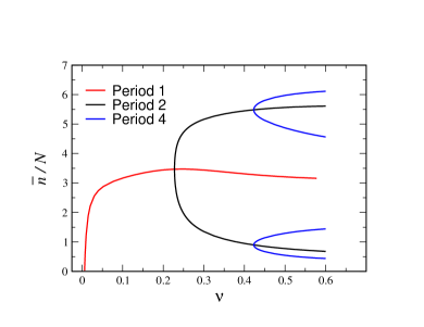
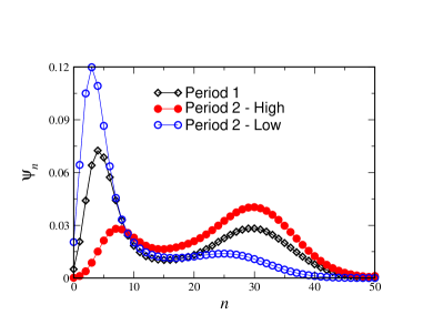
Figure 1: Upper: Solution branches for $N=5$, showing the period 1, 2 and 4 branches as a function of $\nu$. Lower: Probability Distributions $\psi_{n}$ for the period 1 solution at $\nu=0.2$ and for the two phases of the period 2 solution at $\nu=0.25$. The points are connected to guide the eye.

What about the stability of the period-1 solution? The above numerical technique of course only identifies solutions and does not say anything about their stability. One can prove, however, that any periodic orbit must become unstable as $\nu\to 1$. As pointed out by Durrett and Levin durrett , in that case the occupation of a site just before the reaction step is a Poisson distribution with a mean given by the total population in the last step. As a result, $\overline{n}$ satisfies the iterative map,

$$\overline{n}_{t+1}=\sum_{k}kF(k)e^{-\overline{n}_{t}}\frac{(\overline{n}_{t})^{k}}{k!}$$ (4)

where $F$ is the deterministic map. In the Ricker case the resulting map for $\overline{n}$ is also unimodal and the resulting transformation is chaotic in the regime of parameters considered here. Thus any periodic orbit must lose its stability as $\nu$ approaches unity.

All the considerations and the results presented so far are general and are independent of the strength of the stochasticity, which is inversely proportional to $N$. We turn now to consider the differences between strong and weak stochasticity and the semi-deterministic (large $N$) limit.

Let us refer again to Figure 1 where the results for $N=5$ (strong stochasticity) are graphed. There is a range of $\nu$ for which the period 1 is stable, as can be verified by MC simulation. Increasing $\nu$ this time-independent state goes unstable and the system undergoes a forward (supercritical) bifurcation to a period-two state. This state losses stability in favor of a period-4 solution and so on; our results suggest that in that case a cascade of period doubling supercritical bifurcations emerges until, at some $\nu$, there is a transition to global chaos. The period two solution also supports a bimodal distribution, but now the weight of the two peaks are not equal so the overall population takes different value as the peaks switch positions. A similar scenario happens in the period 4 regime.

Comparing our results with the deterministic system discussed in mzm , in the presence of strong demographic noise one may observe the fully synchronized phase (when $\nu$ approaches one and the map shows global chaos) but what about the turbulent phase? This phase appears in the deterministic system when the coupling is too small and different patches oscillate incoherently. Clearly the extinction phase is a consequence of turbulence. However, the transition from the turbulent phase to the cluster phase in the deterministic system occurs at much higher $\nu$ than the extinction transition for the stochastic system (which is exponentially small in $N$). The answer to this puzzle lies in the fact that there is no clear distinction between the cluster phase and the turbulent phase in the stochastic system. As $N$ or $\nu$ are reduced, the distribution broadens and the identifiable peaks wash out. Furthermore the total signal in both phases is time independent. Only in the infinite $N$ limit can a sharp distinction between the two phases be made. In this limit, the distribution function becomes two delta function peaks at infinite $N$ in the cluster phase, and have finite support in the turbulent phase..

Let us now focus our attention on the clustering phase of the deterministic system.. One of the features of this phase is observed here: the system clusters spontaneously into two peaks and the global population follows a periodic orbit. However, there are two important differences: first, in the deterministic system for the same $\nu$ many possible solutions exist, each corresponds to different height ratio between the peaks, while here for any migration parameter only one stable solution survives, so the infinite degeneracy that characterizes the deterministic dynamics disappears. Second, the sharp (delta) peaks of the deterministic solutions are replaced by smooth distributions. One expects, however, that the stochastic system converges to the deterministic one as $N$ increases. How does that happen?

Let us start to increase $N$. For $N=10$ (results not shown) the bifurcation from period 1 to period 2 is backward (subcritical), while the bifurcation from period 2 to period 4 is still forward even at $N=20$. The location of the bifurcation from period 1 to 2 is almost independent of $N$, but the bifurcation from 2 to 4 is strongly $N$ dependent, moving to smaller $\nu$ as $N$ increases. In fact, by $N=40$ it has already moved to the backward branch of the period 2 solution. This situation is summarized in the upper panel of Fig. 2, where the period 1, 2 and 4 solution branches are traced out for $N=60$.

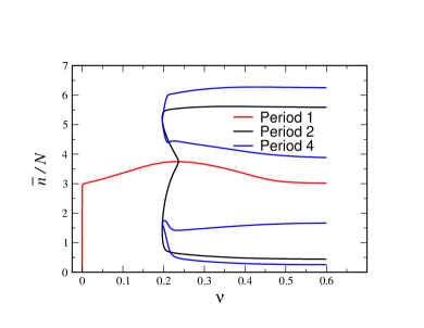
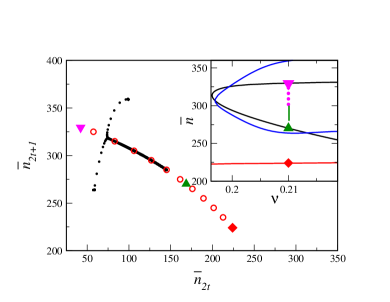
Figure 2: Upper: Solution branches for $N=60$, showing the period 1, 2 and 4 branches as a function of $\nu$. Lower: The return map $\overline{n}_{2t+1}$ versus $\overline{n}_{2t}$, indicated by black dots, for $N=60$, $\nu=0.21$, taken from the simulation depicted in Fig. 3. The trajectory - a drift away from the green triangle, then split to the period 4 orbit - is determined by the line of quasi solutions indicated by the red circles. The triangles represent true period 2 solutions for which $\alpha=0$, and the period 1 solution is indicated by a red diamond. The inset is a blowup of the relevant section of the upper panel, indicating the true solutions and the slow flow through the quasi-solutions. The solutions for $\nu=0.21$ are marked by the same symbols as in the main figure. For these parameters the dynamics close to the green triangle is so slow that measuring the dynamics becomes impractical. When $N\to\infty$, all the region between the green triangle and the splitting point (indicated by full green line in the inset) becomes marginally stable.

The most important issue is how the deterministic continuum of period two solutions is recovered as $N$ grows to infinity. As explained above the period 2 solutions are identified by searching for all pairs of $\lambda_{1},\lambda_{2}$ that admit an invariant eigenvector $\psi$ such that $\lambda_{1}=\sum\psi_{n}F(n)$, and $\lambda_{2}=\sum F(n)\left[{\cal{M}}(\lambda_{1})\psi\right]_{n}$. It turns out that, for large $N$, there is a range of $\lambda_{1}$, $\lambda_{2}$ for which the Markov matrix ${\cal{M}}_{21}\equiv{\cal{M}}(\lambda_{2}){\cal{M}}(\lambda_{1})$ admits, in addition to its invariant eigenvector, an additional eigenstate $\tilde{\psi}$ with an eigenvalue very close to 1, say, $1-\epsilon$. Thus, up to a small term (for $N=80$, e.g., $\epsilon=10^{-12}$) any linear combination of the first and the second eigenvectors imitates the real invariant state until $t\sim 1/\epsilon$. Within this time horizon one has, effectively, a continuous family of invariant eigenvectors of ${\cal{M}}_{21}$, $(1-\alpha)\psi+\alpha\tilde{\psi}$. The two auxiliary conditions no longer are sufficient to determine a solution. We call these solutions for which we ignore $\epsilon$ a quasi-solution, of which there exists a continuous family depending on $\alpha$. It turns out that $\epsilon$ decreases sharply with increasing $N$; the deterministic limit emerges from this continuous family of solutions as explained below.

In Fig. 3, we see all this exemplified in a simulation, where we plotted $\overline{n}_{t}$ as a function of $t$, for $N=60$, $\nu=0.21$. We see that for times less than roughly $5\cdot 10^{5}$, the system exhibits an essentially period 2 type behavior, with an extremely slow drift of the two states. Suddenly, beyond this point, the system converts to a period 4 behavior. A good way of analyzing the drift is to plot $\overline{n}_{2t+1}$ vs. $\overline{n}_{2t}$, as seen in Fig. 2 (lower panel). If the system had a true period 2 orbit, this graph would show a single point. Instead, the drift converts this into a curve. The points on this curve coincide precisely with the above described quasi-solutions, a number of which are indicated by circles. The true solutions are represented by triangles (period 2) and a diamond (period 1) in the figure. The system drifts to larger amplitude oscillations, until the instability is encountered and the it goes to a period 4 orbit, represented by two dots in the figure. While there are quasi-solutions (as well as a true solution $\alpha=0$) beyond this point, they are not dynamically relevant due to their strong instability.

Figure 3: The average population $\overline{n}_{t}$ versus $t$ for $N=60$, $\nu=0.21$. Data obtained by direct integration of the Master equation.

In summary, then, we have seen that adding demographic noise to a globally coupled chaotic map has a marked effect on the dynamics, leading in fact to very regular dynamics for intermediate coupling strength. As the noise strength is reduced, there appears an exponentially long scale, which goes over to the continuous family of solutions seen in the no noise limit.

Beyond the problems considered here, our work suggests a novel mechanism for stochastic-deterministic (”quantum-classical”) correspondence. In general it is assumed that the infinite number of solutions that characterizes the deterministic case emerge from the discrete eigenstates of the stochastic theory when the level spacing approaches zero in the weak stochasticity limit. Here we observed a different scenario, where only two eigenstates provide us with a continuum of deterministic solutions at the $N\to\infty$ limit.

References

- (1) K. Kaneko, Phys. Rev. Lett. 63, 219 (1989); Physica D 41, 137 (1990).
- (2) K. Kaneko, I. Tsuda, Complex systems: Chaos and Beyond (Springer-Verlag, Berlin Heidelberg 2001).
- (3) See a summary in: S.C. Manrubia, A.S. Mikhailov, and D.H. Zanette, Emergence of Dynamical Order: Synchronization Phenomena in Complex Systems (World Scientific, Singapore, 2004).
- (4) For general reviews see Theory and Applications of Coupled Map Lattices, edited by K. Kaneko (Wiley, New York, 1993); A. Pikovsky, M. Rosenblum, and J. Kurths, Synchronization: A Universal Concept in Nonlinear Sciences, (CUP, Cambridge, 2001); S. Boccaletti, V. Latora, Y.Moreno, M. Chaves, and D.-U. Hwang, Physics Reports 424 175, 2006..
- (5) G.F. Gause, The struggle for existence. William and Wilkins, Baltimore (1934); C.B. Huffaker Hilgardia 27 343 (1958); D. Pimentel and W.P. Nagel, Am. Nat., 97, 141 (1963).
- (6) B. Kerr, M.A. Riley, M.W. Feldman and B.J.M. Bohannan, Nature 418, 171 (2002); B. Kerr, C. Neuhauser, B.J.M. Bohannan and A.M. Dean A.M., Nature 442, 75 (2006); M. Holyoak and S.P. Lawler, Ecology 77, 1867 (1996); S. Dey S and A. Joshi, Science 312, 434 (2006).
- (7) R. Durrett and S.A. Levin, Theor. Pop. Biol. 46, 361 (1994).
- (8) M.J. Keeling, H.B. Wilson, S.W. Pacala, Science 290 1758 (2000); T. Reichenbach, M. Mobilia and E. Frey, Nature 448, 1046 (2007), E. Bettelheim, O. Agam and N.M. Shnerb, Physica E 9, 600 (2000).
- (9) D.J.D. Earn, S.A. Levin, P. Rohani, Science 290, 1360 (2000). D.J.D. Earn, S.A. Levin, PNAS 103, 3968 (2006).
- (10) I.A. Hanski and M.E. Gilpin, Metapopulation Biology: Ecology, Genetic and Evolution (Academic Press, San Diego 1997).
- (11) W.E. Ricker, J. Fisheries Res. Board Can., 11 559, 1954.
- (12) W.D. Hamilton, R.M. May, Nature 269, 578 (1977); H.N. Comins, W.D. Hamilton, R.M. May, Journal of Theoretical Biology 82, 205 (1980).