Theory and simulation of two-dimensional nematic and tetratic phases

Abstract

Recent experiments and simulations have shown that two-dimensional systems can form tetratic phases with four-fold rotational symmetry, even if they are composed of particles with only two-fold symmetry. To understand this effect, we propose a model for the statistical mechanics of particles with almost four-fold symmetry, which is weakly broken down to two-fold. We introduce a coefficient $\kappa$ to characterize the symmetry breaking, and find that the tetratic phase can still exist even up to a substantial value of $\kappa$. Through a Landau expansion of the free energy, we calculate the mean-field phase diagram, which is similar to the result of a previous hard-particle excluded-volume model. To verify our mean-field calculation, we develop a Monte Carlo simulation of spins on a triangular lattice. The results of the simulation agree very well with the Landau theory.

I Introduction

In statistical mechanics, one key issue is how the microscopic symmetry of particle shapes and interactions is related to the macroscopic symmetry of the phases. This issue is especially important for liquid-crystal science, where researchers control the orientational order of phases by synthesizing molecules with rod-like, disk-like, bent-core, or other shapes. In many cases, the low-temperature phase has the same symmetry as the particles of which it is composed, while the high-temperature phase has a higher symmetry. For example, in two dimensions (2D), particles with a rectangular or rod-like shape, which has two-fold rotational symmetry, form a low-temperature nematic phase, which also has two-fold symmetry. Likewise, if the particles are perfect squares, which have four-fold rotational symmetry, they can form a four-fold symmetric tetratic phase.

An interesting question is what happens if the symmetry of the particles is slightly broken. Will the symmetry of the phase also be broken, or can the particles still form a higher-symmetry phase? For example, we can consider particles with approximate four-fold rotational symmetry that is slightly broken down to two-fold, as in Fig. 1. Can these particles still form a tetratic phase, or will they only form a less symmetric nematic phase?

Figure 1: Schematic illustration of an interacting particle system in the tetratic phase. The shape of the particles indicates that the rotational symmetry of the interaction is broken down from four-fold to two-fold.

Recently, several experimental and theoretical studies have addressed this problem. Narayan et al. Narayan et al. (2006) performed experiments on a vibrated-rod monolayer, and found that two-fold symmetric rods can form a four-fold symmetric tetratic phase over some range of packing fraction and aspect ratio. Zhao et al. Zhao et al. (2007) studied experimentally the phase behavior of colloidal rectangles, and found what they called an almost tetratic phase. Donev et al. Donev et al. (2006) simulated the phase behavior of a hard-rectangle system with an aspect ratio of 2, and showed they form a tetratic phase. Another simulation by Triplett et al. Triplett and Fichthorn (2008) showed similar results. In further theoretical work, Martínez-Ratón et al. Martínez-Ratón et al. (2005); Martínez-Ratón and Velasco (2009) developed a density-functional theory to study the effect of particle geometry on phase transitions. They found a range of the phase diagram in which the tetratic phase can exist, as long as the shape is close enough to four-fold symmetric. In all of these studies, the particles interact through hard, Onsager-like  Onsager (1949), excluded-volume interactions.

The purpose of the current paper is to investigate whether the same phase behavior occurs for particles with longer-range, soft interactions. We consider a general four-fold symmetric interaction, which is slightly broken down to two-fold symmetry. We first calculate the phase diagram using a Maier-Saupe-like mean-field theory Maier and Saupe (1958, 1959, 1960). To verify the theory, we then perform Monte Carlo simulations for the same interaction.

This work leads to two main results. First, the tetratic phase still exists up to a surprisingly high value of the microscopic symmetry breaking (as characterized by the interaction parameter $\kappa$, which is defined below). Second, the phase diagram is quite similar to that found by Martínez-Ratón et al. for particles with excluded-volume repulsion. This similarity indicates that the phase behavior is generic for particles with almost-four-fold symmetry, independent of the specific interparticle interaction.

The plan of this paper is as follows. In Section II, we present our model and calculate the mean-field free energy. We then examine the phase behavior and calculate the phase diagram in Section III. In Section IV we describe the Monte Carlo simulation methods and results. Finally, in Section V we discuss and summarize the conclusions of this study.

As an aside, we should mention one point of terminology. The tetratic phase has occasionally been called a “biaxial” phase, by analogy with 3D biaxial nematic liquid crystals Martínez-Ratón et al. (2005). However, this analogy is somewhat misleading. In 3D liquid crystals, the word “biaxial” refers to a phase with orientational order in the long molecular axis and in the transverse axes, i.e. a phase with lower symmetry than a conventional uniaxial nematic. By contrast, the tetratic phase has higher symmetry than a conventional nematic, four-fold rather than two-fold. For that reason, we will not use the term “biaxial” in this work.

II Model

Maier-Saupe theory is a widely used form of mean-field theory, which describes the isotropic-nematic transition in 3D liquid crystals. In this section, we extend Maier-Saupe theory to describe 2D liquid crystals with almost-four-fold symmetry, as shown in Fig. 1. For this purpose, we use the modified Maier-Saupe interaction

$$U_{12}\left(r_{12},\theta_{12}\right)=-U_{0}(r_{12})\left[\kappa\cos\left(2\theta_{12}\right)+\cos\left(4\theta_{12}\right)\right],$$ (1)

where $\theta_{12}=\theta_{1}-\theta_{2}$ is the relative orientation angle between particles 1 and 2, and $r_{12}$ is the distance between these particles. In this interaction, the dominant orientation-dependent term is $\cos\left(4\theta_{12}\right)$, which has perfect four-fold symmetry. The term $\cos\left(2\theta_{12}\right)$ represents a correction to the interaction, which has only two-fold symmetry. If the coefficient $\kappa$ is small, then the symmetry is slightly broken from four-fold down to two-fold. (By contrast, if $\kappa$ is large, then the interaction clearly has two-fold symmetry and the four-fold term is unimportant, as in classic Maier-Saupe theory.) The overall coefficient $U_{0}(r_{12})$ is an arbitrary distance-dependent term.

In mean-field theory, we average the interaction energy to obtain an effective single-particle potential due to all the other particles,

$$U_{\textrm{eff}}\left(\theta_{1}\right)=\int\mathrm{d}^{2}{\bf r}_{12}\mathrm{d}\theta_{2}\rho\left(\theta_{2}\right)U_{12}\left(r_{12},\theta_{12}\right).$$ (2)

Here, $\rho\left(\theta_{2}\right)$ is the orientational distribution function, which is normalized as

$$\rho_{0}=\int_{0}^{\pi}\mathrm{d}\theta\rho\left(\theta\right),$$ (3)

where $\rho_{0}$ is the number density of particles. To calculate $U_{\textrm{eff}}$, we set the $x$-axis along an ordered direction (the director in nematic case, or one of the two orthogonal ordered directions in the tetratic case). In that case, the averages of $\sin(2\theta)$ and $\sin(4\theta)$ vanish by symmetry, and hence Eq. (2) becomes

$$U_{\textrm{eff}}\left(\theta\right)=-\bar{U}\rho_{0}\left[\kappa C_{2}\cos\left(2\theta\right)+C_{4}\cos\left(4\theta\right)\right],$$ (4)

where $\bar{U}$ is the integral over the position-dependent part of the potential, and

$$C_{2} = \left<\cos\left(2\theta\right)\right>,$$ (5a)

$$C_{4} = \left<\cos\left(4\theta\right)\right>.$$ (5b)

The resulting orientational distribution function is

$$\rho\left(\theta\right)=\frac{\rho_{0}\exp[\gamma(\kappa C_{2}\cos(2\theta)+C_{4}\cos(4\theta))]}{\int_{0}^{\pi}\mathrm{d}\theta\exp[\gamma(\kappa C_{2}\cos(2\theta)+C_{4}\cos(4\theta))]},$$ (6)

where we have defined the dimensionless ratio $\gamma=\rho_{0}\bar{U}/(k_{B}T)$.

Note that $C_{2}$ can be regarded as a nematic order parameter, and $C_{4}$ as a tetratic order parameter. In the isotropic phase, the system has $C_{2}=C_{4}=0$. By comparison, in the tetratic phase, the system has $C_{2}=0$ but $C_{4}\not=0$. In the nematic phase, with the most order, the system has $C_{2}\not=0$ and $C_{4}\not=0$.

To determine which of these phases is most stable, we must calculate the free energy $F=\left<U\right>+k_{B}T\left<\log\rho\right>$ as a function of the order parameters $C_{2}$ and $C_{4}$. The average interaction energy per particle is

$$\left<U\right>=-\frac{1}{2}\bar{U}\rho_{0}\left(\kappa C_{2}^{2}+C_{4}^{2}\right).$$ (7)

The entropic part of the free energy per particle is

$$k_{B}T\left<\log\rho\right>=\bar{U}\rho_{0}\left(\kappa C_{2}^{2}+C_{4}^{2}\right)$$

$$-k_{B}T\log\left(\frac{1}{\pi}\int_{0}^{\pi}\mathrm{d}\theta\exp[\gamma(\kappa C_{2}\cos 2\theta+C_{4}\cos 4\theta)]\right);$$

here we have have subtracted off the constant entropy of the isotropic phase. We combine these terms and normalize by $k_{B}T$ to obtain the dimensionless free energy

$$\frac{F}{k_{B}T}=\frac{1}{2}\gamma\left(\kappa C_{2}^{2}+C_{4}^{2}\right)$$

$$-\log\left(\frac{1}{\pi}\int_{0}^{\pi}\mathrm{d}\theta\exp[\gamma(\kappa C_{2}\cos 2\theta+C_{4}\cos 4\theta)]\right).$$

Minimizing this free energy with respect to $C_{2}$ and $C_{4}$ gives the equations

$$C_{2} = \frac{1}{\rho_{0}}\int_{0}^{\pi}\mathrm{d}\theta\cos(2\theta)\rho\left(\theta\right),$$ (10a)

$$C_{4} = \frac{1}{\rho_{0}}\int_{0}^{\pi}\mathrm{d}\theta\cos(4\theta)\rho\left(\theta\right),$$ (10b)

which are exactly consistent with Eqs. (5).

(a) (b) (c) (d)

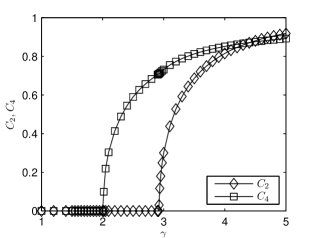
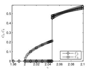
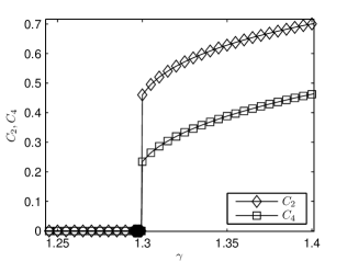
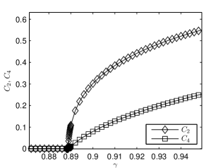
Figure 2: Numerical mean-field calculation of the order parameters $C_{2}$ and $C_{4}$ as functions of $\gamma$ (inverse temperature), for several values of $\kappa$ (two-fold distortion in the interaction): (a) $\kappa=0.4$. (b) $\kappa=0.75$. (c) $\kappa=1.5$. (d) $\kappa=2.25$.

III Mean-field results

The model is now completely defined by two dimensionless parameters: $\gamma=\rho_{0}\bar{U}/(k_{B}T)$ is the ratio of interaction energy to temperature, and $\kappa$ represents the breaking of four-fold symmetry in the interparticle interaction. We would like to determine the phase diagram in terms of these two parameters. As a first step, we minimize the free energy of Eq. (II) numerically using Mathematica. We then do analytic calculations to obtain exact values for second-order transitions and special points in the phase diagram.

Figure 2 shows the numerical mean-field results for the order parameters $C_{2}$ and $C_{4}$ as functions of $\gamma$, for several values of $\kappa$. These plots represent experiments in which the temperature is varied, for particles with a fixed interaction. When the four-fold symmetry is only slightly broken by the small value $\kappa=0.4$, there are two second-order transitions, first from the high-temperature isotropic phase to the intermediate tetratic phase, and then from the tetratic phase to the low-temperature nematic phase. For a larger value $\kappa=0.75$, the isotropic-tetratic transition is still second-order, but now the tetratic-nematic transition is first-order, with a discontinuous change in $C_{2}$. For $\kappa=1.5$, the two transitions merge into a single first-order transition directly from isotropic to nematic, with discontinuities in both $C_{2}$ and $C_{4}$, and the tetratic phase does not occur. Finally, for the largest value $\kappa=2.25$, the isotropic-nematic transition becomes second-order; this behavior corresponds to the prediction of 2D Maier-Saupe theory with a simple $\cos 2\theta_{12}$ interaction.

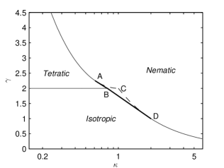
Figure 3: Phase diagram of the model in terms of $\gamma$ (inverse temperature) and $\kappa$ (two-fold distortion in the interaction). The grey solid lines represent second-order transitions, and the dark solid lines are first-order transitions. The dashed lines indicate the extrapolated second-order transitions, which give the cooling limits of the metastable phases. Point B (0.79,2) is the triple point, and A (0.61,2.2) and D (2,1) are the two tricritical points. Point C (1,2) is the intersection of the extrapolated second-order transitions.

The numerical mean-field results are summarized in the phase diagram of Fig. 3. The system has an isotropic phase at low $\gamma$ (high temperature) and a nematic phase at high $\gamma$ (low temperature). It also has an intermediate tetratic phase, as long as the symmetry-breaking $\kappa$ is sufficiently small. The temperature range of the tetratic phase is very large for small $\kappa$, then it decreases as $\kappa$ increases, and finally vanishes at the triple point B. In this mean-field approximation, the isotropic-tetratic transition is always second-order and independent of $\kappa$. The tetratic-nematic transition is second-order for small $\kappa$, then becomes first-order at the tricritical point A. The direct isotropic-nematic transition is second-order for large $\kappa$, then becomes first-order at the tricritical point D. Point C is the intersection of the extrapolated second-order transitions, and represents the limit of metastability of the tetratic phase.

To calculate second-order transitions and special points in the phase diagram, we minimize the free energy of Eq. (II) analytically. For this calculation, we expand the free energy as a power series in the order parameters $C_{2}$ and $C_{4}$, which gives

$$\frac{F}{k_{B}T} = \frac{\gamma\kappa(2-\gamma\kappa)}{8}C_{2}^{2}+\frac{\gamma(2-\gamma)}{4}C_{4}^{2}-\frac{\kappa^{2}\gamma^{3}}{8}C_{2}^{2}C_{4}$$ (11)

$$+\frac{\kappa^{4}\gamma^{4}}{64}C_{2}^{4}+\frac{\gamma^{4}}{64}C_{4}^{4}+\ldots.$$

Note that this expression is exactly what would be expected in a Landau expansion based on symmetry; it is always an even function in $C_{2}$, but it is an even function of $C_{4}$ only when $C_{2}=0$.

To find the isotropic-tetratic transition, we set $C_{2}=0$ in the expansion, because this order parameter vanishes in both of those phases. The second-order isotropic-tetratic transition then occurs when the coefficient of $C_{4}^{2}$ passes through 0. Hence, the transition is at

$$\gamma=2,$$ (12)

independent of $\kappa$.

For the second-order isotropic-nematic transition, we see that the isotropic phase becomes unstable when $\partial^{2}F/\partial C_{2}^{2}=\partial^{2}F/\partial C_{4}^{2}=\partial^{2}F/\partial C_{2}\partial C_{4}=0$, all evaluated at $C_{2}=C_{4}=0$. These equations have two solutions, one of which corresponds to the isotropic-tetratic transition found above. The other solution, representing the isotropic-nematic transition, is

$$\gamma=\frac{2}{\kappa}.$$ (13)

On the nematic side of this transition, we find $C_{4}=\kappa^{2}\gamma^{2}C_{2}^{2}/[4(2-\gamma)]$; i.e. the order parameters $C_{2}$ and $C_{4}$ increase with different critical exponents. We substitute that relation into the expansion (11) to obtain an effective free energy in terms of $C_{2}$ alone,

$$\frac{F_{\textrm{eff}}}{k_{B}T}=\frac{\gamma\kappa(2-\gamma\kappa)}{8}C_{2}^{2}+\frac{\gamma^{4}\kappa^{4}(1-\gamma)}{32(2-\gamma)}C_{2}^{4}+\ldots.$$ (14)

The tricritical point D occurs when the coefficients of both $C_{2}^{2}$ and $C_{2}^{4}$ vanish in this expansion, which is at $\gamma=1$ and $\kappa=2$.

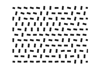
Figure 4: A snapshot of the spins on a triangular lattice in the tetratic phase. The shape of the rectangles is just a schematic illustration of the symmetry of their interaction.

For the second-order tetratic-nematic transition, we cannot use the expansion of Eq. (11) because $C_{4}$ is not necessarily small; instead we return to the free energy of Eq. (II). Anywhere in the tetratic phase we must have $\partial F/\partial C_{4}=0$, which implies

$$C_{4}=\frac{I_{1}(C_{4}\gamma)}{I_{0}(C_{4}\gamma)},$$ (15)

where $I_{0}$ and $I_{1}$ are modified Bessel functions of the first kind. At the tetratic-nematic transition, we also have $\partial^{2}F/\partial C_{2}^{2}=0$, evaluated at $C_{2}=0$, which implies

$$2-\gamma\kappa=\frac{\gamma\kappa I_{1}(C_{4}\gamma)}{I_{0}(C_{4}\gamma)}.$$ (16)

These two equations implicitly determine the second-order tetratic-nematic transition line shown in Fig. 3. To find the tricritical point A, we expand the free energy in powers of $C_{2}$, for $C_{4}$ satisfying Eq. (15), and we require that the coefficients of $C_{2}^{2}$ and $C_{2}^{4}$ both vanish. As a result, the tricritical point A occurs at $\gamma=2.2496$, $\kappa=0.6116$ and $C_{4}=0.4535$.

(a) (b) (c) (d)

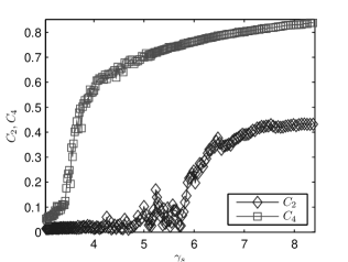
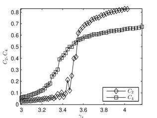
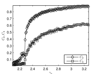
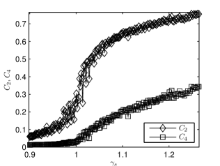
Figure 5: Simulation results for the order parameters $C_{2}$ and $C_{4}$ as functions of $\gamma$ (inverse temperature), for several values of $\kappa$ (two-fold distortion in the interaction): (a) $\kappa=0.3$. (b) $\kappa=0.5$. (c) $\kappa=1$. (d) $\kappa=3$.

The first-order transition lines in the phase diagram cannot be calculated analytically; instead they are determined by numerical minimization of the free energy. The triple point B occurs where the first-order transition lines intersect the second-order isotropic-tetratic transition of Eq. (12). This point is found numerically at $\gamma=2$ and $\kappa=0.79$.

Point C is the intersection of the extrapolated second-order transitions of Eqs. (12) and (13), which occurs at $\gamma=2$ and $\kappa=1$. It represents the highest value of the symmetry breaking $\kappa$ where the tetratic phase can even be metastable, beyond the the triple point B where it ceases to be a stable phase.

IV Monte Carlo simulations

So far, the calculations presented in this paper have all used mean-field theory. Of course, mean-field theory is an approximation, which tends to exaggerate the tendency toward ordered phases. In order to assess the validity of mean-field theory, we perform Monte Carlo simulations for a lattice model of the same system. In this lattice model, we use the Hamiltonian

$$H=-J\sum_{\left<i,j\right>}\left(\kappa\cos[2(\theta_{i}-\theta_{j})]+\cos[4(\theta_{i}-\theta_{j})]\right),$$ (17)

summed over nearest-neighbor sites $i$ and $j$ on a 2D triangular lattice, as shown in Fig. 4. This lattice Hamiltonian corresponds to the model presented in the previous sections if we take the parameter $\gamma=6J/(k_{B}T)$, because each lattice site interacts with six nearest neighbors.

We simulate this model on a lattice of size $100\times 100$ with periodic boundary conditions, using the standard Metropolis algorithm Metropolis et al. (1953). On each lattice site, the spin is described by an orientation angle $\theta$. In each trial Monte Carlo step, a spin is chosen randomly, its orientation is changed slightly, and the resulting change in the energy $\Delta E$ is calculated. If energy decreases, the change is definitely accepted. If not, the change is accepted with a probability of $\exp\left[-\Delta E/(k_{B}T)\right]$. Usually, for a constant temperature, each Monte Carlo cycle of the simulation consists of 10000 trial steps, and 50000 cycles are used for each temperature. However, near phase transitions, especially near first-order transitions, additional Monte Carlo cycles are used to eliminate metastable states. The phase diagram is calculated by cooling the system from high temperature with decreasing the temperature in steps of 0.01, or steps of 0.005 near phase transitions. During the last half of the simulation cycles, the order parameters are calculated and time-averaged.

To calculate the nematic order parameter $C_{2}$, we use the 2D nematic order tensor

$$Q_{\alpha\beta}=2\left(\left<n_{\alpha}n_{\beta}\right>-\left<n_{\alpha}n_{\beta}\right>_{\textrm{iso}}\right),$$ (18)

averaged over all lattice sites. Here, ${\bf n}=(\cos\theta,\sin\theta)$ is the unit vector representing each spin, and $\left<n_{\alpha}n_{\beta}\right>_{\textrm{iso}}=\frac{1}{2}\delta_{\alpha\beta}$ is the average in the isotropic phase. The positive eigenvalue of this tensor is $C_{2}$.

For the tetratic order parameters $C_{4}$, we use the generalized tensor method of Zheng and Palffy-Muhoray Zheng and Palffy-Muhoray (2007). We consider the fourth-order tetratic order tensor

$$T_{\alpha\beta\gamma\delta}=4\left(\left<n_{\alpha}n_{\beta}n_{\gamma}n_{\delta}\right>-\left<n_{\alpha}n_{\beta}n_{\gamma}n_{\delta}\right>_{\textrm{iso}}\right),$$ (19)

averaged over all lattice sites. Here, we are subtracting off the isotropic average $\left<n_{\alpha}n_{\beta}n_{\gamma}n_{\delta}\right>_{\textrm{iso}}=\frac{1}{8}(\delta_{\alpha\beta}\delta_{\gamma\delta}+\delta_{\alpha\gamma}\delta_{\beta\delta}+\delta_{\alpha\delta}\delta_{\beta\gamma})$. To calculate the eigenvalues, we unfold this fourth-order tensor into a second-order tensor ($4\times 4$ matrix), which we diagonalize using standard methods. The four eigenvalues are $0$, $-C_{4}$, $\frac{1}{2}\left(C_{4}-(16C_{2}^{2}+C_{4}^{2})^{1/2}\right)$, and $\frac{1}{2}\left(C_{4}+(16C_{2}^{2}+C_{4}^{2})^{1/2}\right)$. (In the tetratic phase, with $C_{2}=0$, they reduce to $0$, $-C_{4}$, $+C_{4}$, and $0$.) Thus, using the previously calculated value of $C_{2}$, we can extract $C_{4}$.

Figure 5 shows the simulation results for the order parameters $C_{2}$ and $C_{4}$ as functions of $\gamma$, for several values of $\kappa$. These results are quite simular to the numerical mean-field results of Fig. 2, although the quantitative values of $\gamma$, $\kappa$, and the order parameters are somewhat different. For a small symmetry breaking $\kappa=0.3$, there are two second-order phase transitions. The order parameter $C_{4}$ increases continuously at the high-temperature isotropic-tetratic transition, and $C_{2}$ increases continuously at the lower-temperature tetratic-nematic transition. For a slightly larger value of $\kappa=0.5$, the tetratic-nematic transition becomes first-order, with an apparently discontinuous increase in $C_{2}$ (within the precision of the simulation). For $\kappa=1$, the intermediate tetratic phase disappears, and there is just a single first-order isotropic-nematic transition, with apparently discontinuous increases in both $C_{2}$ and $C_{4}$. Finally, for the largest value $\kappa=3$, the isotropic-nematic transition becomes second-order, with continuous increases in both $C_{2}$ and $C_{4}$.

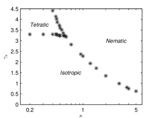
Figure 6: Simulation results for the phase diagram in terms of $\gamma$ (inverse temperature) and $\kappa$ (two-fold distortion in the interaction). The triple point is at approximately $\gamma=3.2$ and $\kappa=0.60$.

The simulation results are summarized in the phase diagram of Fig. 6. This phase diagram shows a high-temperature isotropic phase, an intermediate tetratic phase, and a low-temperature nematic phase. The temperature range of the tetratic phase is very large when the symmetry breaking $\kappa$ is small, then it decreases as $\kappa$ increases, and eventually vanishes at the triple point, which is approximately given by $\gamma=3.2$ and $\kappa=0.60$. Compared with the mean-field phase diagram of Fig. 3, the simulation results show the transitions at lower temperature (higher $\gamma$) than in mean-field theory. This difference is reasonable because mean-field theory always exaggerates the tendency toward ordered phases.

V Conclusions

In this paper, we propose a model for the statistical mechanics of particles with almost-four-fold symmetry. In contrast with earlier work on particles with a hard-core excluded-volume interaction, we consider particles with a soft interaction, analogous to Maier-Saupe theory of nematic liquid crystals. We investigate this model through two complementary techniques, mean-field calculations and Monte Carlo simulations. Both of these techniques predict a phase diagram with a low-temperature nematic phase, an intermediate tetratic phase, and a high-temperature isotropic phase. They make consistent predictions for the order of the transitions and the temperature dependence of the order parameters, although they do not agree in all quantitative details.

The main result of this study is that the tetratic phase can exist up to a surprisingly high value of the symmetry breaking $\kappa$ in the microscopic interaction. We find the maximum $\kappa=0.79$ in mean-field theory, or 0.60 in Monte Carlo simulations. Even taking the lower Monte Carlo value, this implies that the interaction in the parallel direction $(1+\kappa)$ can be about four times larger than the interaction in the perpendicular direction $(1-\kappa)$. Hence, the tetratic phase can form even for particles with quite a substantial two-fold component in the interaction energy, i.e. for fairly rod-like particles.

It is interesting to note that our phase diagram is quite similar to the phase diagram found by density-functional theory for hard rectangles; see Fig. 3 of Ref. Martínez-Ratón et al. (2005). In that theory, the phase diagram shows isotropic, tetratic, and nematic phases, and the tetratic phase can exist for rectangles with aspect ratio of up to 2.21:1. That theory shows the same arrangement of the phases, and even the same first- and second-order phase transitions, with tricritical points on the isotropic-nematic and tetratic-nematic transition lines. This phase diagram seems to be a generic feature of particles with four-fold symmetry broken down to two-fold. Thus, we can expect to see tetratic phases in 2D experiments and simulations, even if the particles are moderately extended.