Non-linear spin wave theory results for the frustrated $S=\frac{1}{2}$ Heisenberg antiferromagnet on a body-centered cubic lattice

Abstract

At zero temperature the sublattice magnetization of the quantum spin-$1/2$ Heisenberg antiferromagnet on a body-centered cubic lattice with competing first and second neighbor exchange ($J_{1}$ and $J_{2}$) is investigated using the non-linear spin wave theory. The zero temperature phases of the model consist of a two sublattice Néel phase for small $J_{2}$ (AF₁) and a collinear phase at large $J_{2}$ (AF₂). We show that quartic corrections due to spin-wave interactions enhance the sublattice magnetization in both the AF₁ and the AF₂ phase. The magnetization corrections are prominent near the classical transition point of the model and in the $J_{2}>J_{1}$ regime. The ground state energy with quartic interactions is also calculated. It is found that up to quartic corrections the first order phase transition (previously observed in this model) between the AF₁ and the AF₂ phase survives.

I Introduction

In recent years thermodynamic properties of frustrated quantum Heisenberg antiferromagnets have been of intense interest both theoretically and experimentally in condensed matter physics. Diep (2004); Sachdev (2001) The phase diagram of the quantum spin-$1/2$ Heisenberg antiferromagnetic (AF) model on two-dimensional (2D) lattices with nearest neighbor ($J_{1}$) and next nearest neighbor interactions ($J_{2}$) have been studied extensively by different methods. Rastelli et al. (1979); Reatto and Tassi (1985); Sachdev ; Sachdev (1992); Harris et al. (1992); Dotsenko and Sushkov (1994); Huse and Rutenberg (1992); Chubukov (1992); Chubukov et al. (1994); Gelfand et al. (1989); Sushkov et al. (2001); Weihong et al. (1999); Singh et al. (1999); Starykh and Balents (2004); Kotov et al. (1999); An et al. (2001); Honda et al. (2002); Svistov and et. al ; Gochev (1994) For the square lattice with nearest neighbor (NN) exchange interaction only, the ground state is antiferromagnetically ordered at zero temperature. Addition of next nearest neighbor (NNN) interactions break the AF order. The competition between the NN and NNN interactions for the square lattice is characterized by the frustration parameter $p$. It has been found that a quantum spin liquid phase exists between $p_{1c}\approx 0.38$ and $p_{2c}\approx 0.60$. For $p<p_{1c}$ the lattice is AF-ordered whereas for $p>p_{2c}$ a collinear phase emerges. In the collinear state the NN spins have a parallel orientation in the vertical direction and antiparallel orientation in the horizontal direction or vice versa.

Motivated by the results for the 2D lattices some work has been done by analytical and numerical techniques to understand the magnetic phase diagram of three dimensional (3D) lattices. Oguchi et al. (1985); Ignatenko et al. (2008); Oitmaa and Zheng (2004); Schmidt et al. (2002); Viana et al. (2008) Linear spin-wave theory, exact diagonalization, and linked-cluster series expansions (both at zero and finite temperature) have been utilized to study the 3D quantum spin-$1/2$ Heisenberg AF on a body-centered-cubic lattice (bcc) lattice. Schmidt et al. (2002); Oitmaa and Zheng (2004) It has been found that the lattice does not have a quantum disordered phase and a first-order phase transition from the AF-phase (AF₁) to lamellar state (AF₂) occurs at $p_{c}=0.53$ or J₂/J${}_{1}\approx$ 0.705. The first-order nature of the phase transition from the AF₁ to the AF₂ phase in the model is inferred from a kink in the ground state energy of the system. In one and 2D due to reduced phase space quantum fluctuations play an important role in determining the quantum critical points of the system at low temperature. However, in 3D the phase space available is greater and quantum fluctuations play a lesser role. Hence, the absence of the quantum disordered phase for the BCC lattice.

In this work, we study the 3D quantum spin-$1/2$ AF on a bcc lattice using the non-linear spin wave theory where we consider interactions between spin waves up to quartic terms in the Hamiltonian. We compute the effect of these higher order terms on the sublattice magnetization (see Fig 2). The corrections to the magnetization become important as the classical transition point p_c=0.5 is approached. Also, our calculations re-confirm the first order nature of the phase transition found in Refs. Schmidt et al., 2002; Oitmaa and Zheng, 2004 up to quartic interactions (see Fig 3).

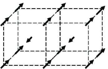
(a)  AF₁ phase

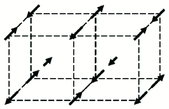
(b)  AF₂ phase

Figure 1: AF₁ and AF₂ ordered phases of the bcc lattice. In the AF₁ phase all $A$-sublattice spins point in the direction of an arbitrary unit vector while $B$-sublattice spins point in the opposite direction. For the AF₂ phase there are two interpenetrating Néel states each living on the initial sublattices $A$ and $B$.

The paper is organized as follows. In Section II we begin with a brief description of the properties of the bcc lattice relevant to our calculations. We then set-up the Hamiltonian for the Heisenberg spin-$1/2$ AF on the bcc lattice. The classical ground state configurations of the model and the different phases are then discussed. Next we map the spin Hamiltonian to the Hamiltonian of interacting bosons and the non-linear spin-wave theory for the two phases are developed. The sublattice magnetizations and the ground state energies for the two phases are numerically calculated and the results are plotted and discussed in Section III. Finally we summarize our results in Section IV.

II Formalism

Body-centered-cubic lattice consists of two interpenetrating, identical simple cubic lattices, each of which consists of two interpenetrating, identical face-centered lattices. This makes the bcc lattice a 3D bi-bipartite cubic lattice. The basis vectors of the bcc lattice connecting eight ($z_{1}=8$) nearest neighbors are (in units of simple cubic lattice spacing) ${\bf a_{1}}=(1,1,-1),\;{\bf a_{2}}=(1,-1,1),\;{\bf a_{3}}=(-1,1,1)$ and the lattice vectors connecting six ($z_{2}=6$) next-nearest neighbors are ${\bf b_{1}}=(\pm 2,0,0),\;{\bf b_{2}}=(0,\pm 2,0)$ and ${\bf b_{3}}=(0,0,\pm 2)$. On such a lattice the Hamiltonian for a spin-$1/2$ Heisenberg AF with first and second neighbor interactions is

$$H=\frac{1}{2}J_{1}\sum_{\langle ij\rangle}{\bf S}_{i}\cdot{\bf S}_{j}+\frac{1}{2}J_{2}\sum_{[ij]}{\bf S}_{i}\cdot{\bf S}_{j}.$$ (1)

where $J_{1}$ is the NN and $J_{2}$ is the frustrating NNN exchange constants. Both couplings are considered AF, i.e. $J_{1},J_{2}>0$.

II.1 Classical ground state configurations

The limit of infinite spin, $S\rightarrow\infty$ corresponds to the classical Heisenberg model. We assume that the set of possible spin configurations of the system are described by $S_{i}=S{\bf u}e^{i{\bf q}\cdot{\bf r_{i}}}$, where ${\bf u}$ is a vector expressed in terms of an arbitrary orthonormal basis and ${\bf q}$ defines the relative orientation of the spins on the lattice. Villain (1959) The classical ground state energy of the system expressed as a function of the parameters $J_{1}$ and $J_{2}$ takes the form

$$E_{\bf k}/NJ_{1}=\frac{1}{2}S^{2}z_{1}[\gamma_{1{\bf k}}+p\gamma_{2{\bf k}}],$$ (2)

with the structure factors

$$\gamma_{1{\bf k}} = \cos(k_{x})\cos(k_{y})\cos(k_{z}),$$ (3)

$$\gamma_{2{\bf k}} = \Big{[}\cos(2k_{x})+\cos(2k_{y})+\cos(2k_{z})\Big{]}/3.$$ (4)

where $N$ is the number of sites on the lattice and $p=z_{2}J_{2}/z_{1}J_{1}$ is defined to be the parameter of frustration.

At zero temperature, the classical ground state for the bcc lattice has two phases. In the limit of small $p$ or $J_{2}<<J_{1}$ three isolated minima in energy, $E_{0}/NJ_{1}=-4S^{2}(1-p)$ occur at the wave-vectors $(\pi,0,0),(0,\pi,0)$ and $(0,0,\pi)$. They correspond to the classical two-sublattice Néel state (AF₁ phase) where all $A$-sublattice spins point in the direction of an arbitrary unit vector ${\bf{\hat{n}}}$ while $B$-sublattice spins point in the opposite direction $-{\bf{\hat{n}}}$.

In the other limit, for large $p$ or $J_{2}>>J_{1}$, there is a single minimum in energy, $E_{0}/NJ_{1}=-4S^{2}p$ at ${\bf k}=(\pi/2,\pi/2,\pi/2)$. In this case the classical ground state consists of two interpenetrating Néel states (AF₂ phase) each living on the initial sublattices $A$ and $B$. The two phases are shown in Fig. 1.

The classical limit for the phase transition from AF₁ to AF₂ for the 3D model on the bcc lattice is at the critical value $p_{c}=2z_{2}/3z_{1}=1/2$ i.e. when $J_{2}/J_{1}=2/3$. This is similar to the spin-$1/2$ $J_{1}-J_{2}$ model on a 2D square lattice where the critical value of $p_{c}=1/2$ or $J_{2}/J_{1}=1/2$.

II.2 Non-linear spin wave theory

The Hamiltonian in Eq. 1 can be mapped into an equivalent Hamiltonian of interacting bosons by transforming the spin operators to bosonic operators $a,a^{\dagger}$ for $A$ sublattice and $b,b^{\dagger}$ for $B$ sublattice using the well-known Holstein-Primakoff transformations Holstein and Primakoff (1940)

$$S_{Ai}^{+} \approx \sqrt{2S}\Big{(}1-\frac{a_{i}^{\dagger}a_{i}}{4S}\Big{)}a_{i},\;\;S_{Ai}^{-}\approx\sqrt{2S}a_{i}^{\dagger}\Big{(}1-\frac{a_{i}^{\dagger}a_{i}}{4S}\Big{)},$$

$$S_{Ai}^{z} = S-a^{\dagger}_{i}a_{i},$$

$$S_{Bj}^{+} \approx \sqrt{2S}b_{j}^{\dagger}\Big{(}1-\frac{b_{j}^{\dagger}b_{j}}{4S}\Big{)},\;\;S_{Bj}^{-}\approx\sqrt{2S}\Big{(}1-\frac{b_{j}^{\dagger}b_{j}}{4S}\Big{)}b_{j},$$

$$S_{Bj}^{z} = -S+b^{\dagger}_{j}b_{j},$$ (5)

In these transformations we have kept terms up to the order of $1/S$. Next using the Fourier transforms

$$a_{i}=\sqrt{\frac{2}{N}}\sum_{\bf k}e^{-i{\bf k\cdot R_{i}}}a_{\bf k},\;\;\;b_{j}=\sqrt{\frac{2}{N}}\sum_{\bf k}e^{-i{\bf k\cdot R_{j}}}b_{\bf k},$$

the real space Hamiltonian is transformed to the ${\bf k}$-space Hamiltonian. The reduced Brillouin zone contains $N/2$ ${\bf k}$ vectors as the unit cell is a magnetic supercell consisting of an $A$-site and a $B$-site. In the following two sections we study the cases $J_{2}<J_{1}$ and $J_{2}>J_{1}$ separately.

II.2.1 $J_{2}<J_{1}$: AF₁ phase

In this phase the classical ground state is the two-sublattice Néel state (see Fig. 1). For the NN interaction spins in $A$ sublattice interacts with spins in $B$ sublattice and vice-versa. On the other hand for the NNN exchange $J_{2}$ connects spins on the same sublattice $A$ with $A$ and $B$ with $B$. Substituting Eq. 5 in Eq. 1, expanding the radical, and restricting to terms only up to the anharmonic quartic terms, we obtain the ${\bf k}$-space Hamiltonian

$$H=H^{(0)}+H^{(2)}+H^{(4)}.$$ (6)

The classical ground state energy $H^{(0)}$ and the quadratic terms $H^{(2)}$ are

$$H^{(0)} = -\frac{1}{2}NJ_{1}S^{2}z_{1}(1-p)$$ (7)

$$H^{(2)} = J_{1}Sz_{1}\sum_{\bf k}\Big{[}A_{0{\bf k}}(a_{\bf k}^{\dagger}a_{\bf k}+b_{\bf k}^{\dagger}b_{\bf k})$$ (8)

$$+ B_{0{\bf k}}(a^{\dagger}_{\bf k}b^{\dagger}_{-\bf k}+a_{-\bf k}b_{\bf k})\Big{]},$$

with the coefficients $A_{0{\bf k}}$ and $B_{0{\bf k}}$ defined as

$$A_{0{\bf k}} = 1-p(1-\gamma_{2{\bf k}}),$$ (9)

$$B_{0{\bf k}} = \gamma_{1{\bf k}}.$$ (10)

The quartic terms in the Hamiltonian $H^{(4)}$ are

$$H^{(4)} = -J_{1}\sum_{\langle ij\rangle}\Big{[}a_{i}^{\dagger}a_{i}b^{\dagger}_{j}b_{j}+\frac{1}{4}\Big{(}a_{i}b^{\dagger}_{j}b_{j}b_{j}+a_{i}^{\dagger}a_{i}a_{i}b_{j}+h.c.\Big{)}\Big{]}$$ (11)

$$+ \frac{1}{2}J_{2}\sum_{[ij]}\Big{[}a^{\dagger}_{i}a_{i}a^{\dagger}_{j}a_{j}-\frac{1}{4}\Big{(}a_{i}a^{\dagger}_{j}a_{j}^{\dagger}a_{j}+a_{i}^{\dagger}a_{i}a_{i}a_{j}^{\dagger}+h.c.\Big{)}$$

$$+ a\leftrightarrow b\Big{]}.$$

These terms are evaluated by applying the Hartree-Fock decoupling process. Chernyshev and Zhitomirsky In the harmonic approximation the following Hartree-Fock averages are non-zero for the bcc-lattice Heisenberg AF:

$$u = \langle a_{i}^{\dagger}a_{i}\rangle=\langle b_{i}^{\dagger}b_{i}\rangle=\frac{1}{2}\Big{[}\frac{2}{N}\sum_{\bf k}\frac{A_{0{\bf k}}}{\omega_{0{\bf k}}}-1\Big{]},$$ (12)

$$v = \langle a_{i}b_{j}\rangle=\langle a_{i}^{\dagger}b_{j}^{\dagger}\rangle=-\frac{1}{2}\Big{[}\frac{2}{N}\sum_{\bf k}\frac{\gamma_{1{\bf k}}B_{0{\bf k}}}{\omega_{0{\bf k}}}\Big{]},$$ (13)

$$w = \langle a_{i}^{\dagger}a_{j}\rangle=\langle b_{i}^{\dagger}b_{j}\rangle=\frac{1}{2}\Big{[}\frac{2}{N}\sum_{\bf k}\frac{\gamma_{2{\bf k}}A_{0{\bf k}}}{\omega_{0{\bf k}}}\Big{]},$$ (14)

where $\omega_{0{\bf k}}=\sqrt{A_{0{\bf k}}^{2}-B_{0{\bf k}}^{2}}.$

The contributions of the decoupled quartic terms to the harmonic Hamiltonian in Eq. 8 are to renormalize the values of $A_{0{\bf k}}$ and $B_{0{\bf k}}$ which are now

$$A_{\bf k} = \Big{(}1-\frac{u+v}{S}\Big{)}-p[1-\gamma_{2{\bf k}}]\Big{(}1-\frac{u-w}{S}\Big{)},$$ (15)

$$B_{\bf k} = \gamma_{1{\bf k}}\Big{(}1-\frac{u+v}{S}\Big{)},$$ (16)

$$\omega_{\bf k} = \sqrt{A_{\bf k}^{2}-B_{\bf k}^{2}}.$$ (17)

The quartic corrections to the ground state energy is calculated from the four-boson averages. In the leading order they are decoupled into the bilinear combinations (Eqs. 12 – 14) using Wick’s theorem. The corresponding four boson terms are,

$$\langle a^{\dagger}_{i}a_{i}b^{\dagger}_{j}b_{j}\rangle = u^{2}+v^{2},\;\;\;\langle a^{\dagger}_{i}b^{\dagger}_{j}b_{j}b_{j}\rangle=2uv,$$

$$\langle a^{\dagger}_{i}a_{i}a_{i}b_{j}\rangle = 2uv,\;\;\;\langle a^{\dagger}_{i}a_{i}a_{j}^{\dagger}a_{j}\rangle=u^{2}+w^{2},$$ (18)

$$\langle a_{i}a_{j}^{\dagger}a_{j}^{\dagger}a_{j}\rangle = 2uw,\;\;\;\langle a^{\dagger}_{i}a_{i}a_{i}a_{j}^{\dagger}\rangle=2uw.$$

This yields the ground state energy correction from the quartic terms

$$\delta E^{(4)}=-\frac{1}{2}NJ_{1}z_{1}\Big{[}(u+v)^{2}-p(u-w)^{2}\Big{]}.$$ (19)

Summing all the corrections together the ground state energy takes the form

$$E/NJ_{1} = -\frac{1}{2}z_{1}S(S+1)(1-p)+\frac{1}{2}z_{1}S\Big{[}\frac{2}{N}\sum_{\bf k}\omega_{\bf k}\Big{]}$$

$$+ \frac{1}{2}z_{1}\Big{[}(u+v)(1-u-v)-p(u-w)(1-u+w)\Big{]}.$$

and the sublattice magnetization $\langle S_{\alpha}\rangle$ at zero temperature is given by

$$\langle S_{\alpha}\rangle=S\Big{[}1-\frac{1}{2S}\Big{\{}\frac{2}{N}\sum_{\bf k}\frac{A_{\bf k}}{\omega_{\bf k}}-1\Big{\}}\Big{]}.$$ (21)

Using Eqs. 15, 16, and  17 we numerically evaluate $E/NJ_{1}$ and $\langle S_{\alpha}\rangle$. For the bcc lattice the k-sum is replaced by an integral over the Brillouin zone Flax and Raich (1969)

$$\frac{2}{N}\sum_{\bf k}\rightarrow\frac{1}{\pi^{3}}\int_{0}^{\pi}\int_{0}^{\pi}\int_{0}^{\pi}\;dk_{x}dk_{y}dk_{z}.$$ (22)

II.2.2 $J_{2}>J_{1}$: AF₂ phase

The classical ground state for $J_{2}>J_{1}$ corresponds to a four sublattice state where each of the $A$ and $B$ sublattice is itself antiferromagnetically ordered (see Fig. 1). For the NN exchange there are four $A-A$, four $B-B$, and eight $A-B$ type interactions between the sublattices. In case of NNN exchanges there are a total of twelve $A-B$ type interactions. Adding all their contributions together up to the quadratic terms the harmonic Hamiltonian takes the same form as Eq. 8 with

$$H^{(0)} = -\frac{1}{2}NJ_{1}S^{2}z_{1}p,$$ (23)

$$A_{0{\bf k}} = \frac{1}{2}(\gamma_{1{\bf k}}+2p),$$ (24)

$$B_{0{\bf k}} = \frac{1}{2}(\gamma_{1{\bf k}}+2p\gamma_{2{\bf k}}).$$ (25)

The quartic terms in the Hamiltonian for this case are

$$H^{(4)} = -J_{1}\sum_{\langle ij\rangle}\Big{[}a_{i}^{\dagger}a_{i}b^{\dagger}_{j}b_{j}+\frac{1}{4}\Big{(}a_{i}b^{\dagger}_{j}b_{j}b_{j}+a_{i}^{\dagger}a_{i}a_{i}b_{j}+h.c.\Big{)}\Big{]}$$ (26)

$$+ \frac{1}{2}J_{1}\sum_{\langle ij\rangle}\Big{[}a^{\dagger}_{i}a_{i}a^{\dagger}_{j}a_{j}-\frac{1}{4}\Big{(}a_{i}a^{\dagger}_{j}a_{j}^{\dagger}a_{j}+a_{i}^{\dagger}a_{i}a_{i}a_{j}^{\dagger}+h.c.\Big{)}$$

$$+ a\leftrightarrow b\Big{]}-J_{2}\sum_{\langle ij\rangle}\Big{[}a_{i}^{\dagger}a_{i}b^{\dagger}_{j}b_{j}+\frac{1}{4}\Big{(}a_{i}b^{\dagger}_{j}b_{j}b_{j}+a_{i}^{\dagger}a_{i}a_{i}b_{j}$$

$$+ h.c.\Big{)}\Big{]}.$$

These terms are decoupled and evaluated in the same way as before. The renormalized values of the coefficients $A_{\bf k}$ and $B_{\bf k}$ are

$$A_{\bf k} = \frac{1}{2}\Big{[}\gamma_{1{\bf k}}\Big{(}1-\frac{u-{\overline{w}}}{S}\Big{)}-\frac{v+{\overline{w}}}{S}+2p\Big{(}1-\frac{u+{\overline{v}}}{S}\Big{)}\Big{]},$$

$$B_{\bf k} = \frac{1}{2}\Big{[}\gamma_{1{\bf k}}\Big{(}1-\frac{u+v}{S}\Big{)}+2p\gamma_{2{\bf k}}\Big{(}1-\frac{u+{\overline{v}}}{S}\Big{)}\Big{]},$$ (28)

where

$${\overline{v}} = -\frac{1}{2}\Big{[}\frac{2}{N}\sum_{\bf k}\frac{\gamma_{2{\bf k}}B_{0{\bf k}}}{\omega_{0{\bf k}}}\Big{]},$$ (29)

$${\overline{w}} = \frac{1}{2}\Big{[}\frac{2}{N}\sum_{\bf k}\frac{\gamma_{1{\bf k}}A_{0{\bf k}}}{\omega_{0{\bf k}}}\Big{]}.$$ (30)

In Eqs. II.2.2 and 28 $u,v$ have the same form as in Eqs. 12 – 13 but they are evaluated with the coefficients $A_{0\bf k}$ and $B_{0\bf k}$ in Eqs. 24 and  25. The quartic corrections to the ground state energy is

$$\delta E^{(4)}=\frac{1}{2}NJ_{1}z_{1}\Big{\{}(u-{\overline{w}})^{2}-(u+v)^{2}-p(u+{\overline{v}})^{2}\Big{\}}.$$ (31)

Combining all these corrections the ground state energy is

$$E/NJ_{1} = -\frac{1}{2}z_{1}S(S+1)p+\frac{1}{2}z_{1}S\Big{[}\frac{2}{N}\sum_{\bf k}\omega_{\bf k}\Big{]}$$ (32)

$$+ \frac{1}{4}z_{1}\Big{[}(v+{\overline{w}})(1-2u-v+{\overline{w}})$$

$$+ 2p(u+{\overline{v}})(1-u-{\overline{v}})\Big{]}.$$

The sublattice magnetization and ground state energy are then obtained numerically using Eqs. 21, II.2.2, 28, and 32.

III Results

In Fig. 2 we show the results for the sublattice magnetization, $\langle S_{\alpha}\rangle$, obtained numerically from Eq. 21 for both AF₁ and AF₂ phases with (dashed line) and without (solid line) quartic corrections. In the AF₁ ordered phase or the two sublattice Néel phase where $A$ and $B$ sublattice spins point in the opposite directions, sublattice magnetization decreases monotonically with increase in $p$ till $p\approx 0.5$. The curve starts at $\approx 0.44$ for $p=0$ and ends at $\approx 0.34$ for $p=0.5$. The gradual decrease in $\langle S_{\alpha}\rangle$ is expected with increase in $p$ as increasing strength of NNN interaction $J_{2}$ aligns the spins antiferromagnetically along the horizontal and the vertical directions. The quartic corrections produce a change in the sublattice magnetization, $\langle S_{\alpha}\rangle$, which becomes significant as one approaches the classical transition point p_c=0.5 (see Fig. 2). With quartic corrections the magnetization curve starts at $\approx 0.44$ for $p=0$ and ends at $\approx 0.38$ for $p=0.49$. At $p=0$ (no frustration) there is no quartic corrections to $\langle S_{\alpha}\rangle$. This can be observed from Eqs. 15– 17, 21 as the correction factor $(1-(u+v)/S)$ cancels out in Eq. 21. At the wave-vector ${\bf k}=(\pi/2,\pi/2,\pi/2)$ spin-wave theory calculations become unstable (at $p_{c}\approx 0.5$) since the coefficient $A_{{\bf k}}$ becomes equal to $B_{{\bf k}}$.

Figure 2: Sublattice magnetization, $\langle S_{\alpha}\rangle$, is plotted versus $p$ for AF₁ and AF₂ ordered phases. In the AF₁ phase with increase in $p$ the system aligns the spins antiferromagnetically along the horizontal and the vertical directions – thus decreasing the sublattice magnetization. In the AF₂ phase $\langle S_{\alpha}\rangle$ mostly stays the same and then shows a slight decrease (without quartic corrections) as $p$ approaches the critical value $p_{c}=0.5$ from above. However with the quartic corrections $\langle S_{\alpha}\rangle$ remains almost constant at $\approx 0.43$. In both cases quartic corrections to the Hamiltonian of the system enhance the magnetic order.

Figure 3: Ground state energy per site, E/NJ₁, is plotted as a function of the frustration parameter $p=z_{2}J_{2}/z_{1}J_{1}$ without (solid lines) and with (dashed lines) quartic corrections for both AF₁ ($p<0.5$) and AF₂ ($p>0.5$) ordered phases. For the bcc-lattice $z_{1}=8$ and $z_{2}=6$. Spin wave theory becomes unstable at the classical transition point, i.e. $p\approx 0.5$. After extrapolation (not indicated in the figure above) we find that the two energies meet at $p\approx 0.53$ or $J_{2}/J_{1}\approx 0.705$. The kink in the energy at this value of $p$ indicates a first order quantum phase transition from AF₁ to AF₂ phase.

In the AF₂ ordered phase or the lamellar phase with two interpenetrating Néel states, sublattice magnetization stays mostly flat except for a slight decrease (without quartic corrections) as $p$ approaches the critical value $p_{c}$ from above. The curve starts at $\approx 0.42$ for $p=1$ and ends at $\approx 0.41$ for $p=0.5$. However with quartic corrections the curve has a very small upward turn. This upward curve has been observed in previous numerical works on this model. Oitmaa and Zheng (2004); Schmidt et al. (2002) For the AF₂ phase, quartic fluctuations produce an overall enhancement of the magnetization over the high-$p$ values (0.5 to 1). But for low-$p$ (0 to 0.5), with increase in frustration quantum spin fluctuations play a dominant role as seen in Fig. 2.

In Fig. 3 we plot the ground state energy per site, E/NJ₁, for the AF₁ and AF₂ phases with and without quartic corrections as a function of the frustration parameter $p=z_{2}J_{2}/z_{1}J_{1}$. $p_{c}=0.5$ is the classical transition point where a phase transition from the AF₁ phase to the AF₂ phase occur. The quadratic calculation agrees well with the results of  Oitmaa and Zheng, 2004; Schmidt et al., 2002. The quartic corrections to the energy are shown by the dashed lines in Fig. 3. At $p=0$ calculated energy with the quartic correction is slightly lower than the energy calculated without the quartic interaction terms. This small decrease from the linear spin wave theory calculation is due to the ground state energy correction which is negative (as seen in Eq. 19) from the quartic terms (self-energy Hartree diagrams). This trend for low-$p$ continues till $p\approx 0.38$ after which the energy with quartic corrections become dominant. For large $p$, we find the energy with quartic corrections to be lower than the energy calculated without the quartic interactions in the interval $\approx 0.70-1$. In both the phases quantum spin fluctuations tend to maintain the magnetic order by lowering the ground state energies. As $p$ approaches the critical value $p_{c}$ from both phases, frustration increases causing the ground state energies to increase. Then $1/S$ corrections due to spin fluctuations play a lesser role. As mentioned in the magnetization calculation our non-linear spin wave analysis becomes unstable at the classical transition point $p_{c}=0.5$. After extrapolation of the ground state energy curve from the AF₁ phase in the regime where non-linear spin wave theory breaks down we find that the energies from the two phases meet at $p\approx 0.53$. not The kink at this point signals a first-order phase transition occurs from AF₁ to AF₂ phase.

IV Conclusions

In this work we have investigated the zero temperature $1/S$ corrections to the sublattice magnetization and ground state energy of a spin-$1/2$ Heisenberg frustrated antiferromagnet on a bcc lattice using the framework of non-linear spin wave theory. We have found that $1/S$ corrections due to spin-wave interactions cause noticeable changes to the sublattice magnetization for both the two sublattice Néel phase (small NNN interaction $J_{2}$) and the AF₂ phase or the lamellar phase (large $J_{2}$). As non-linear spin wave theory calculations become unstable close to the classical transition point we are unable to analyze the nature of phase transition using this method. We also confirm that up to quartic corrections the system undergoes a first-order phase transition as indicated by a kink in the energy calculation.

V Acknowledgment

One of us (K.M.) thanks O. Starykh for helpful discussions.

References

- Diep (2004) H. T. Diep, Frustrated Spin Systems (World Scientific, Singapore, 2004), 1st ed.
- Sachdev (2001) S. Sachdev, Quantum Phase Transitions (Cambridge University Press, Cambridge, UK, 2001), 1st ed.
- Rastelli et al. (1979) E. Rastelli, A. Tassi, and L. Reatto, Physica 97B, 1 (1979).
- Reatto and Tassi (1985) E. R. L. Reatto and A. Tassi, J. Phys. C: Solid State Phys. 18, 353 (1985).
- (5) S. Sachdev, eprint cond-matstr-el/0901.4103.
- Sachdev (1992) S. Sachdev, Phys. Rev. B 45, 12 377 (1992).
- Harris et al. (1992) A. B. Harris, C. Kallin, and A. J. Berlinsky, Phys. Rev. B 45, 2899 (1992).
- Dotsenko and Sushkov (1994) A. V. Dotsenko and O. Sushkov, Phys. Rev. B 50, 13 821 (1994).
- Huse and Rutenberg (1992) D. A. Huse and A. D. Rutenberg, Phys. Rev. B 45, 7536 (1992).
- Chubukov (1992) A. Chubukov, Phys. Rev. Lett. 69, 832 (1992).
- Chubukov et al. (1994) A. Chubukov, S. Sachdev, and T. Senthil, J, Phys.: Condens. Matter 6, 8891 (1994).
- Gelfand et al. (1989) M. P. Gelfand, R. R. P. Singh, and D. A. Huse, Phys. Rev. B 40, 10801 (1989).
- Sushkov et al. (2001) O. P. Sushkov, J. Oitmaa, and Z. Weihong, Phys. Rev. B 63, 104420 (2001).
- Weihong et al. (1999) Z. Weihong, R. H. McKenzie, and R. R. P. Singh, Phys. Rev. B 59, 14 367 (1999).
- Singh et al. (1999) R. R. P. Singh, Z. Weihong, C. J. Hammer, and J. Oitmaa, Phys. Rev. B 60, 7278 (1999).
- Starykh and Balents (2004) O. Starykh and L. Balents, Phys. Rev. Lett. 93, 127202 (2004).
- Kotov et al. (1999) V. N. Kotov, J. Oitmaa, O. P. Sushkov, and Z. Weihong, Phys. Rev. B 60, 14613 (1999).
- An et al. (2001) J. An, C.-D. Gong, and H.-Q. Lin, J. Phys.: Condens. Matter 13, 115 (2001).
- Honda et al. (2002) Z. Honda, K. Katsumata, and K. Yamada, J. Phys.: Condens. Matter 14, L625 (2002).
- (20) L. E. Svistov and et. al, eprint cond-mat.str-el/0603617.
- Gochev (1994) I. G. Gochev, Phys. Rev. B 49, 9594 (1994).
- Oguchi et al. (1985) T. Oguchi, H. Nishimori, and Y. Taguchi, J. Phys. Soc. Japan 54, 4494 (1985).
- Ignatenko et al. (2008) A. N. Ignatenko, A. A. Katanin, and V. Y. Irkhin, JETP Letts. 87, 1 (2008).
- Oitmaa and Zheng (2004) J. Oitmaa and W. Zheng, Phys. Rev. B 69, 064416 (2004).
- Schmidt et al. (2002) R. Schmidt, J. Schulenburg, and J. Richter, Phys. Rev. B 66, 224406 (2002).
- Viana et al. (2008) J. R. Viana, J. R. de Sousa, and M. Continentino, Phys. Rev. B 77, 172412 (2008).
- Villain (1959) J. Villain, J. Phys. Chem. Solids 11, 303 (1959).
- Holstein and Primakoff (1940) T. Holstein and H. Primakoff, Phys. Rev. 58, 1098 (1940).
- (29) A. L. Chernyshev and M. E. Zhitomirsky, eprint cond-mat.str-el/0901.4803.
- Flax and Raich (1969) L. Flax and J. Raich, Phys. Rev. 185, 797 (1969).
- (31) To avoid confusion we have not shown the extrapolated line in Fig. 3.