The scalar complex potential of the electromagnetic field

Abstract

In this paper, we define a scalar complex potential $\mathcal{S}$ for an arbitrary electromagnetic field. This potential is a modification of the two scalar potential functions introduced by E. T. Whittaker. By use of a complexified Minkowski space $M$, we decompose the usual Lorentz group representation on $M$ into a product of two commuting new representations. These representations are based on the complex Faraday tensor. For a moving charge and for any observer, we obtain a complex dimensionless scalar which is invariant under one of our new representations. The scalar complex potential is the logarithm of this dimensionless scalar times the charge value. We define a conjugation on $M$ which is invariant under our representation. We show that the Faraday tensor is the derivative of the conjugate of the gradient of the complex potential. The real part of the Faraday tensor coincides with the usual electromagnetic tensor of the field.

The potential $\mathcal{S}$, as a complex-valued function on space-time, is described as an integral over the distribution of the charges generating the electromagnetic field. This potential is like a wave function description of the field. If we chose the Bondi tetrad (called also Newman-Penrose basis) as a basis on $M$, the components of the Faraday vector at each point may be derived from $\mathcal{S}$ by $F_{j}=E_{j}+iB_{j}={\partial}^{\nu}(\alpha_{j})_{\nu}^{\lambda}{\partial}_{\lambda}\mathcal{S}$, where $(\alpha_{j})$ are the known $\alpha$-matrices of Dirac. This fact indicates that our potential may build a ”bridge” between classical and quantum physics.

PACS: 02.30.EM;02.90.+p; 03.50.De .

Keywords: Whittaker potential; retarded potential; complexified Minkowski space; Lorentz group representations, Bondi tetrad; electromagnetic field; wave function of a field; Faraday vector.

I Introduction

In general, the electromagnetic field tensor ${F}$, expressed by a $4\times 4$ antisymmetric matrix, is used to describe the electromagnetic field intensity. This tensor provides a convenient expression for the Lorentz force and therefore is used to describe the motion of charged particles in this field. Another way to describe an electromagnetic field is by use of the 4-potential. In a chosen gauge, the 4-potential transforms as a 4-vector. The electromagnetic field tensor is defined as the derivative of the 4-potential.

In 1904 E. T. Whittaker introduced Whittaker two scalar potential functions. He showed that the electromagnetic field can be expressed in terms of the second derivatives of these functions. H. S. Ruse improved Ruse the result of Whittaker and showed that these two functions transform as invariants. We show that it is possible to combine these two scalar potential functions into one complex-valued function $\mathcal{S}$ on complexified Minkowski space, which we call the scalar complex potential of the electromagnetic field.

Complexified space-time was also used by Barut Barut for introducing a classical theory of fields and particles. In FriedmanPoinc this space was used for different representations of the Poincaré group on relativistic phase space and in FS and F04 for the description of the motion of a charge in an electromagnetic field. It turns out to be easer to express and calculate the scalar complex potential of the electromagnetic field by the use of a Bondi tetrad for complexified Minkowski space. Such a basis is used widely, see for example PenroseRindler , ODonnell . The connection of the relativistic phase space to the Bondi tetrad is described in FriedmanNP . We use the complex Faraday tensor $\mathcal{F}$, which was introduced in Silberstein1 and used in Silberstein2 and FD . The real part of this tensor coincides with the usual electromagnetic tensor of the field. The additional symmetries of this tensor make it attractive to solve evolution equations and to obtain new representations of the Lorentz group.

An electromagnetic field is generated by a collection of moving charges. Thus, a description of an electromagnetic field can be obtained by integrating the fields of moving charges. We show that for a moving charge and observer point in space-time, there is a complex dimension-less scalar which is invariant under some representation of the Lorentz group. The scalar complex potential $\mathcal{S}$ is defined to be the logarithm of this scalar. We show that the Faraday tensor $\mathcal{F}$ is an appropriately defined second order derivative of the scalar complex potential.

In classical mechanics, the negative of the gradient of a scalar potential equals the force. This is true for forces which generate linear acceleration. Such forces are defined by a one-form (since their line integral gives the work). The derivative of a scalar function is also a one-form. Hence, the derivative of a potential could be equal to the negative of the force. But in classical mechanics we also have rotating forces, which are described by two-forms. Such forces cannot be expressed as derivatives of a scalar potential. In special relativity, the electromagnetic field is expressed by a two-form. So, it is natural to assume that a kind of second derivative of a scalar potential will define the force. Note that the usual differential form derivative of a gradient is zero. Therefore, we define a Lorentz invariant conjugation on the complex space-time. We show that the derivative of the conjugate of the gradient of the complex potential equals the Faraday tensor $\mathcal{F}$ of the field.

In Section 2 we recall the definition of the Bondi tetrad on the complexified Minkowski space $M$ and the transformation from the usual basis to it. In Section 3 we introduce a complex Faraday tensor and define the complex analog of the $curl$ operator on $M$. In Section 4 we show that this tensor is decomposable if we use Bondi tetrad for $M$. The Faraday tensor is used in Section 5 to define two Lorentz group representations on the complexified space-time. For each representation we define a conjugation on $M$ which is invariant under it. In section 6 we introduce an invariant scale-free scalar associated with a null-vector. The logarithm of this scalar becomes the scalar complex potential of a moving charge. This potential is introduced in section 7. In Section 8 we calculate the 4-potential of a moving charge as the conjugate of the gradient of the complex potential. In Section 9 we derive the Faraday tensor $\mathcal{F}$ of the field of a moving charge as the derivative of the 4-potential. We give an explicit formula for such a field. In Section 10 we show how to extend the scalar complex potential to arbitrary electromagnetic field. We show that it satisfies the wave equation and obtain an explicit form of the complex $curl$ operator under this representation.

II Complexified Minkowski space with a Bondi tetrad

Let $K$ be an inertial reference frame with basis $\{\mathbf{e}_{\mu}\}$, for $\mu=0,1,2,3,$ and coordinates $(ct,x,y,z)=x^{\mu},$ where $c$ denotes the speed of light. For the rest of the paper we will use units in which $c=1$ and thus we will omit $c$ from equations. Greek indices range over $\{0,1,2,3\}$ and Latin indices over $\{1,2,3\}$. The inner product of two 4-vectors is defined, as usual, as

$$\mathbf{a}\cdot\mathbf{b}=\eta_{\mu\nu}a^{\mu}b^{\nu},\;\;\eta_{\mu\nu}=diag(1,-1,-1,-1).$$ (1)

The space of 4-vectors with this inner product is Minkowski space-time. We now complexify Minkowski space-time by allowing the coefficients $x^{\mu}$ to be complex numbers. As a space this is equivalent to $\mathbf{C}^{4}$. We extend the inner product (1) to a symmetric complex bilinear form. We will call such a space with such a bilinear form on it the complexified Minkowski space and denote it by $M$.

One possible interpretation of $M$ is the following: Consider the state space of a zero spin particle which is described by a complex-valued function $\psi$ on the space-time. The gradient operator, describing a generalized momentum, maps the space-time into $M$ since $\nabla\psi\in\mathbf{C}^{4}$ and the inner product (1) on $M$ is induced from the inner product on space-time. Another possible interpretation of $M$ is: An electromagnetic field is described by a two-tensor $F_{\mu\nu}$ defining the action of the field on the 4-velocity $u^{\mu}$ of a test charge $q$, expressed by equation $\frac{m}{q}\frac{dU^{\mu}}{d\tau}=F^{\mu}_{\nu}U^{\nu}$. The 4-velocity can be considered as a tangent vector to the path of the charge in Minkowski space-time. A typical charge is a collection of electrons. So, we can think of a test charge as a single electron. But a state of an electron describing its evolution depends also on the spin $S$ of the electron, as can be seen from the Stern-Gerlach experiment. The evolution of the spin in the field is given by the BMT equation which, if we assume that the Land$\grave{e}$ factor of the electron to be equal 2, is $\frac{m}{q}\frac{dS^{\mu}}{d\tau}=F^{\mu}_{\nu}S^{\nu}$. Note that the spin evolution is the same as the evolution of the 4-velocity. By complexifying the tangent space of Minkowski space-time, we can define a complex 4-vector $x^{\mu}=U^{\mu}+iS^{\mu}$ that will describe the state of the electron and the space $M$ containing all such state vectors. With this notation the evolution equation will become $\frac{m}{q}\frac{dx^{\mu}}{d\tau}=F^{\mu}_{\nu}x^{\nu}$. Note that since $S$ is a pseudo-vector and $U$ is a vector, in order that $x$ will be well defined $i$ must be a pseudo-scalar which changes its sign with the change of orientation in space. For other possible interpretations of $M$, see also F04 and FriedmanPoinc .

The Bondi null tetrad ( BT , in short), called also Newman-Penrose basis, on $M$ is defined by

$$\mathbf{n}_{0}=\mathbf{n}=\frac{1}{\sqrt{2}}(\mathbf{e}_{0}+\mathbf{e}_{3}),\;\mathbf{n}_{1}=\bar{\mathbf{m}}=\frac{1}{\sqrt{2}}(\mathbf{e}_{1}-i\mathbf{e}_{2}),\;$$

$$\mathbf{n}_{2}=\mathbf{m}=\frac{1}{\sqrt{2}}(\mathbf{e}_{1}+i\mathbf{e}_{2}),\;\mathbf{n}_{3}=\mathbf{l}=\frac{1}{\sqrt{2}}(\mathbf{e}_{0}-\mathbf{e}_{3}).$$ (2)

For the significance of the BT see PenroseRindler , ODonnell and FriedmanNP . Note that application of complex conjugation on $M$, which is equivalent to replacing $i$ with $-i$, maps the BT into itself, but exchanges $\mathbf{n}_{1}$ with $\mathbf{n}_{2}$. This mean that also here $i$ is a pseudo-scalar which with the change of orientation, that may be expressed by change of the order of the basis vectors, changes its sign.

We will denote by $y^{\mu}$ the coordinates of a vector in $M$ with respect to the BT, meaning $x^{\mu}\mathbf{e}_{\mu}=y^{\mu}\mathbf{n}_{\mu}.$ Then, the relation between the coordinates is

$$x^{0}=\frac{1}{\sqrt{2}}(y^{0}+y^{3}),\;x^{1}=\frac{1}{\sqrt{2}}(y^{1}+y^{2}),\;x^{2}=i\frac{1}{\sqrt{2}}(y^{2}-y^{1}),\;x^{3}=\frac{1}{\sqrt{2}}(y^{0}-y^{3}),$$ (3)

or inversely,

$$y^{0}=\frac{1}{\sqrt{2}}(x^{0}+x^{3}),\;y^{1}=\frac{1}{\sqrt{2}}(x^{1}+ix^{2}),\;y^{2}=\frac{1}{\sqrt{2}}(x^{1}-ix^{2}),\;y^{3}=\frac{1}{\sqrt{2}}(x^{0}-x^{3}).$$ (4)

The coordinate transformation could be expressed by the transfer matrix $L=L_{j}^{k}$ given by

$$L=\frac{1}{\sqrt{2}}\left(\begin{array}[]{cccc}1&0&0&1\\ 0&1&i&0\\ 0&1&-i&0\\ 1&0&0&-1\\ \end{array}\right),\;\;L^{-1}=\frac{1}{\sqrt{2}}\left(\begin{array}[]{cccc}1&0&0&1\\ 0&1&1&0\\ 0&-i&i&0\\ 1&0&0&-1\\ \end{array}\right).$$ (5)

Thus,

$$y^{\nu}=L_{\mu}^{\nu}x^{\mu},\;\;x^{\nu}=(L^{-1})_{\mu}^{\nu}y^{\mu}\,.$$ (6)

The metric tensor $\eta$ in the BT is given by

$$\tilde{\eta}=\left(\begin{array}[]{cccc}0&0&0&1\\ 0&0&-1&0\\ 0&-1&0&0\\ 1&0&0&0\\ \end{array}\right)=\tilde{\eta}^{-1}.$$ (7)

The bilinear symmetric scalar product of two 4-vectors $\mathbf{a}=a^{\mu}\mathbf{n}_{\mu}$ and $\mathbf{b}=b^{\mu}\mathbf{n}_{\mu}$ is given by

$$\mathbf{a}\cdot\mathbf{b}=\tilde{\eta}_{\mu\nu}a^{\mu}b^{\nu}.$$

This, for example, implies that

$$(\mathbf{a})^{2}=\mathbf{a}\cdot\mathbf{a}=0\;\;\Leftrightarrow\;\;a^{0}a^{3}=a^{1}a^{2}\;\;\Leftrightarrow\;\;\frac{a^{2}}{a^{0}}=\frac{a^{3}}{a^{1}}\;\;\Leftrightarrow\;\;\frac{a^{1}}{a^{0}}=\frac{a^{3}}{a^{2}}\,.$$ (8)

In case $a^{0}=0$, the last identities need to be reversed $\frac{a^{0}}{a^{2}}=\frac{a^{1}}{a^{3}},\;\frac{a^{0}}{a^{1}}=\frac{a^{2}}{a^{3}}.$ In these coordinates, the lowering of indices is denoted by $a_{\mu}=\tilde{\eta}_{\mu\nu}a^{\nu}$. For example,

$$y_{0}=y^{3},\;\;y_{1}=-y^{2},\;\;y_{2}=-y^{1},\;\;y_{3}=y^{0}.$$ (9)

III Operator Representation of the Faraday Vector

An electromagnetic field can be defined by an electric field intensity $\mathbf{E}(\mathbf{r},t)$ and a magnetic field intensity $\mathbf{B}(\mathbf{r},t)$. Equivalently, one can define a complex 3D-vector, called the Faraday vector, as

$$\mathbf{F}=\mathbf{E}+i\mathbf{B}$$ (10)

in order to represent the electromagnetic field. Note that since $i$ is a pseudo-scalar and $\mathbf{B}$ is a pseudo-vector, the expression $i\mathbf{B}$ is a vector which is independent of the chosen orientation of the space. The Faraday vector is used to describe the Lorentz invariant field constants. See, for example, Landau .

An alternative way to describe an electromagnetic field is by use of the 4-potential $A=A_{\mu}$. It is known that the 4-potential $A=A_{\mu}$ and the $j=1,2,3$ components of the electric and the magnetic field intensities $\mathbf{E},\mathbf{B}$ are connected by

$$E_{j}=\frac{\partial A_{0}}{\partial x^{j}}-\frac{\partial A_{j}}{\partial x^{0}}=A_{0,j}-A_{j,0},\;\;B_{j}=\varepsilon_{j}^{kl}\frac{\partial A_{k}}{\partial x^{l}}=\varepsilon_{j}^{kl}A_{k,l}\,,$$ (11)

where $\varepsilon^{klj}$ denotes the antisymmetric 3D Levi-Civita tensor, with $\varepsilon^{123}=-1$. From this we get that the components of the Faraday vector satisfy

$$F_{j}=E_{j}+iB_{j}=\frac{\partial A_{0}}{\partial x^{j}}-\frac{\partial A_{j}}{\partial x^{0}}+i\varepsilon_{j}^{kl}\frac{\partial A_{k}}{\partial x^{l}}.$$ (12)

We introduce matrices

$$(K_{1})_{\nu}^{\mu}=\frac{1}{2}\left(\begin{array}[]{cccc}0&1&0&0\\ 1&0&0&0\\ 0&0&0&-i\\ 0&0&i&0\\ \end{array}\right),\;(K_{2})_{\nu}^{\mu}=\frac{1}{2}\left(\begin{array}[]{cccc}0&0&1&0\\ 0&0&0&i\\ 1&0&0&0\\ 0&-i&0&0\\ \end{array}\right),\;(K_{3})_{\nu}^{\mu}=\frac{1}{2}\left(\begin{array}[]{cccc}0&0&0&1\\ 0&0&-i&0\\ 0&i&0&0\\ 1&0&0&0\\ \end{array}\right)$$ (13)

and differential operators ${\partial}_{\mu}=(\frac{\partial}{\partial x^{0}}\frac{\partial}{\partial x^{1}}\frac{\partial}{\partial x^{2}}\frac{\partial}{\partial x^{3}})=\frac{\partial}{\partial x^{\mu}}$ and ${\partial}^{\mu}=\eta^{\mu\nu}{\partial}_{\nu}$. With this notation we can rewrite equation (12) as

$$F_{j}=-2{\partial}^{\nu}(K_{j})^{\mu}_{\nu}A_{\mu}.$$ (14)

In FD we introduce a complex Faraday tensor for the description of an electromagnetic field. This tensor is a complex matrix (mixed tensor)

$$\mathcal{F}^{\beta}_{\alpha}=\frac{1}{2}\left(\begin{array}[]{cccc}0&F_{1}&F_{2}&F_{3}\\ F_{1}&0&-iF_{3}&iF_{2}\\ F_{2}&iF_{3}&0&-iF_{1}\\ F_{3}&-iF_{2}&iF_{1}&0\\ \end{array}\right)=\sum_{j=1}^{3}F_{j}(K_{j})^{\beta}_{\alpha}\,,$$ (15)

with $F_{j}$ are defined by (10).

Substituting (14) into (15) we introduce a differential operator

$$(\nabla_{c}\times)^{\beta\mu}_{\alpha}=\sum_{j=1}^{3}(K_{j})_{\alpha}^{\beta}{\partial}^{\nu}(K_{j})^{\mu}_{\nu}.$$ (16)

This operator plays the role of a complex $curl$ on $M$ since

$$\mathcal{F}_{\alpha}^{\beta}=-(\nabla_{c}\times)^{\beta\mu}_{\alpha}A_{\mu}\,.$$

IV Complex Faraday tensor in BT

We will need the representation of the Faraday tensor in BT. We will denote by $\widetilde{\mathcal{F}}$ the matrix of $\mathcal{F}$ in this representation. By the usual formula of basis transformation we get

$$\widetilde{\mathcal{F}}^{\beta}_{\alpha}=L\mathcal{F}^{\beta}_{\alpha}L^{-1}=\frac{1}{2}\left(\begin{array}[]{cccc}F_{3}&F_{1}-iF_{2}&0&0\\ F_{1}+iF_{2}&-F_{3}&0&0\\ 0&0&F_{3}&F_{1}-iF_{2}\\ 0&0&F_{1}+iF_{2}&-F_{3}\\ \end{array}\right).$$ (17)

This show that the Faraday tensor become decomposable in BT. Thus it can be simplified if we introduce the following tensor decomposition.

The tensor decomposition of a $4\times 4$ matrix as a tensor product of $2\times 2$ matrices is defined by use of the binary representation of numbers. Each of our indices $\mu=0,1,2,3$ can be considered as a pair of indices $(\mu_{0},\mu_{1})$ with value in $\mu_{k}\in\{0,1\}$ by

$$0\longmapsto 00,\;\;1\longmapsto 01,\;\;2\longmapsto 10,\;\;3\longmapsto 11\,.$$

The tensor decomposition of a two tensor $D=D_{jk}$ is defined by

$$D=a\otimes b,\;\;D_{\mu\nu}=D_{(\mu_{0},\mu_{1})(\nu_{0},\nu_{1})}=a_{\mu_{0}\nu_{0}}\,b_{\mu_{1}\nu_{1}}\,.$$ (18)

For example, the tensor $\tilde{\eta}$ can be decomposed as $\tilde{\eta}=\left(\begin{array}[]{cc}0&1\\ -1&0\\ \end{array}\right)\otimes\left(\begin{array}[]{cc}0&1\\ -1&0\\ \end{array}\right):=\tilde{\eta}_{2}\otimes\tilde{\eta}_{2}\,.$

The following properties of the tensor decomposition can be verified directly from the definition:

$$a\otimes(b+c)=(a\otimes b)+(a\otimes c),\;\;F(a\otimes b)=(Fa)\otimes b=a\otimes Fb$$ (19)

and

$$(a\otimes b)(c\otimes d)=ac\otimes bd,$$ (20)

where $a,b,c,d$ are $2\times 2$ matrices and $F$ is a constant.

With this notation and the properties of the tensor decomposition, we can rewrite (17) as

$$\widetilde{\mathcal{F}}^{\beta}_{\alpha}=I_{2}\otimes\sum_{j}F_{j}\frac{1}{2}\sigma_{j}=\sum_{j}F_{j}\widetilde{K}_{j},$$ (21)

where $\sigma_{j}$ denote the usual Pauli matrices, and $I_{2}$ is the $2\times 2$ identity matrix. The matrices $K_{j}$ in BT therefore become

$$(\widetilde{K}_{j})^{\mu}_{\nu}=I_{2}\otimes\frac{1}{2}\sigma_{j}.$$ (22)

Formula (14) becomes

$$F_{j}=-2\tilde{\partial}^{\nu}(\tilde{K}_{j})^{\mu}_{\nu}\tilde{A}_{\mu}=-\tilde{\partial}^{\nu}(I_{2}\otimes\sigma_{j})^{\mu}_{\nu}\tilde{A}_{\mu},$$ (23)

where $\tilde{\partial}_{\mu}=(\frac{\partial}{\partial y^{0}}\frac{\partial}{\partial y^{1}}\frac{\partial}{\partial y^{2}}\frac{\partial}{\partial y^{3}})=\frac{\partial}{\partial y^{\nu}}$, $\tilde{\partial}^{\mu}=\tilde{\eta}^{\mu\nu}\tilde{\partial}_{\nu}=\left(\begin{array}[]{c}\tilde{\partial}_{3}\\ -\tilde{\partial}_{2}\\ -\tilde{\partial}_{1}\\ \tilde{\partial}_{0}\\ \end{array}\right)$ and $\tilde{A}_{\mu}$ is the representation of ${A}_{\mu}$ in BT.

The analog of the differential operator $curl$ becomes

$$(\widetilde{\nabla}_{c}\times)^{\beta\mu}_{\alpha}=\sum_{j=1}^{3}2(\tilde{K}_{j})_{\alpha}^{\beta}{\tilde{\partial}}^{\nu}(\tilde{K}_{j})^{\mu}_{\nu}\,$$ (24)

and

$$\widetilde{\mathcal{F}}_{\alpha\beta}=(\widetilde{\nabla}_{c}\times)^{\beta\mu}_{\alpha}\tilde{A}_{\mu}\,.$$ (25)

The complex Faraday tensor $\mathcal{F}^{\beta}_{\alpha}$ defined by (15) is an extension of usual electromagnetic tensor $F^{\beta}_{\alpha}$ in the following way:

$$F^{\beta}_{\alpha}=2Re\mathcal{F}^{\beta}_{\alpha}=\mathcal{F}^{\beta}_{\alpha}+(\mathcal{F}^{*})^{\beta}_{\alpha}\,,$$ (26)

where $(\mathcal{F}^{*})^{\beta}_{\alpha}$ denote the complex conjugate of $\mathcal{F}^{\beta}_{\alpha}$. In BT, the tensor $(\mathcal{F}^{*})^{\beta}_{\alpha}$ becomes

$$(\widetilde{\mathcal{F}}^{*})^{\beta}_{\alpha}=L\mathcal{F}^{*}L^{-1}=\sum_{j}\bar{F}_{j}\frac{1}{2}\sigma^{*}_{j}\otimes I_{2}\,.$$ (27)

¿From this, (21) and (20) it follows that

$$[\mathcal{F},\mathcal{F}^{*}]=0\,.$$ (28)

V Representations of the Lorentz group on $M$

In the previous section we used both the complex Faraday tensor $\mathcal{F}^{\beta}_{\alpha}$ and the usual electromagnetic tensor $F^{\beta}_{\alpha}$ to describe the electromagnetic field action on the complexified Minkowski space $M$. As it was shown in FriedmanPoinc , such operators may be considered as elements of the action of Lie algebra of the Lorentz group on $M$. An electric field, which is connected to acceleration, can be considered as the generator of a boost, and a magnetic field can be considered as the generator of a rotation. Thus, by use of the above operators we can introduce 3 representations of the Lorentz group: $\tilde{\pi}$ based on $\mathcal{F}^{\beta}_{\alpha}$, $\tilde{\pi}^{*}$ based on $(\mathcal{F}^{*})^{\beta}_{\alpha}$ and $\pi$ based on $F^{\beta}_{\alpha}$ on $M$.

We define first the representation $\tilde{\pi}$. A generator $\xi$ of a boost $B_{k}$ in direction $\mathbf{k}=(k_{1},k_{2},k_{3})$ with $|\mathbf{k}|=1$, can be identified with an electric field $\mathbf{E}=(k_{1},k_{2},k_{3})$. Using the BT for $M$, from (10) and (21), we can represent this generator on $M$ as $\xi=I_{2}\otimes\sum k_{j}\frac{1}{2}\sigma_{j}$. Thus, the representation $\tilde{\pi}$ of the boost $B_{k}$ , using (19) and (20), is

$$\tilde{\pi}(B_{k})=\exp(\xi\psi)=\exp((I_{2}\otimes\sum k_{j}\frac{1}{2}\sigma_{j})\psi)=I_{2}\otimes\exp(\sum k_{j}\sigma_{j}\frac{\psi}{2})$$

for some constant $\psi$. Using the fact that $(\sum k_{j}\sigma_{j})^{2}=I_{2}$, we get

$$\tilde{\pi}(B_{k})=I_{2}\otimes\left(\begin{array}[]{cc}\cosh\frac{\psi}{2}+k_{3}\sinh\frac{\psi}{2}&(k_{1}-ik_{2})\sinh\frac{\psi}{2}\\ (k_{1}+ik_{2})\sinh\frac{\psi}{2}&\cosh\frac{\psi}{2}-k_{3}\sinh\frac{\psi}{2}\\ \end{array}\right)$$ (29)

A generator $\eta$ of a rotation $R_{k}$ about the direction $\mathbf{k}=(k_{1},k_{2},k_{3})$, with $|\mathbf{k}|=1$, can be identified with a magnetic field $\mathbf{B}=(k_{1},k_{2},k_{3})$.Using the BT for $M$, from (10) and (21), we can represent this generator on $M$ as $\eta=I_{2}\otimes i\sum k_{j}\frac{1}{2}\sigma_{j}.$ Thus, the representation $\tilde{\pi}$ of the rotation $R_{k}$ , using (19) and (20), is

$$\tilde{\pi}(R_{k})=\exp(\eta\varphi)=\exp((I_{2}\otimes i\sum k_{j}\frac{1}{2}\sigma_{j})\varphi)=I_{2}\otimes\exp(i\sum k_{j}\sigma_{j}\frac{\varphi}{2})$$

for some constant $\varphi$. Since $i(\sum k_{j}\sigma_{j})^{2}=-I_{2}$, we get

$$\tilde{\pi}(R_{k})=I_{2}\otimes\left(\begin{array}[]{cc}\cos\frac{\varphi}{2}+k_{3}i\sin\frac{\varphi}{2}&(ik_{1}+k_{2})\sin\frac{\varphi}{2}\\ (ik_{1}-k_{2})\sin\frac{\varphi}{2}&\cos\frac{\varphi}{2}-k_{3}i\sin\frac{\varphi}{2}\\ \end{array}\right)$$ (30)

for some constant $\varphi.$ Thus, we have a full description of the representation $\tilde{\pi}$ of the Lorentz group on $M$.

To obtain the representation $\pi$ based on the usual electromagnetic tensor $F^{\beta}_{\alpha}$, we use (26) expressing the connection of this tensor to the complex Faraday tensor. For boost $B_{k}$ in direction $\mathbf{k}$, using (26) and (28) we get

$$\pi(B_{k})=\exp\left((\xi+\xi^{*})\psi\right)=\exp\left(\xi\psi\right)\exp\left(\xi^{*}\psi\right)=\tilde{\pi}(B_{k})\tilde{\pi}^{*}(B_{k}).$$ (31)

This defines the usual representation of a boost on the Minkowski space. Similarly, one can check that $\pi(R_{k})$ defines the usual representation of a rotation on Minkowski space.

Note that all our representations are reducible. For representation $\pi$, the real and imaginary parts of $M$ are invariant. The operation of complex conjugation preserving $ReM$ and reversing $ImM$, So that the complex conjugate $y^{*}$ of a vector of $M$ is $y^{*}=Re\,y-iIm\,y$. This conjugation commutes with, and is invariant under, the representation $\pi$. Similarly, for representation $\tilde{\pi}$, from (29) and (30) there are two invariant subspaces $M_{1}=span\{\mathbf{n}_{0},\mathbf{n}_{1}\}$ and $M_{2}=span\{\mathbf{n}_{2},\mathbf{n}_{3}\}$. As a result, we introduce a conjugation, denoted by $y^{\#}$, defined by the action of an operator $J$

$$J=\left(\begin{array}[]{cc}1&0\\ 0&-1\\ \end{array}\right)\otimes I_{2},\;\Rightarrow\;(y^{0},y^{1},y^{2},y^{3})^{\#}=(y^{0},y^{1},-y^{2},-y^{3})$$ (32)

which preserves $M_{1}$ and reverses $M_{2}$. This conjugation replaces the complex conjugation for the representation $\pi$. It commutes with, and is invariant under, the representation $\tilde{\pi}$. A similar conjugation exists also for the representation $\tilde{\pi}^{*}$.

VI Lorentz invariant scale-free scalar associated with a null-vector

Claim Let $a$ be a null-vector with coordinates $a^{\mu}$ in the NP-basis. Then, the dimension-less constant $\zeta=\frac{a^{2}}{a^{0}}$ is an invariant scalar with respect to representation $\tilde{\pi}$ on $M$.

This constant coincides with the “single complex parameter” occurring during the stereographic projection of the celestial sphere to the Agrand plane (see PenroseRindler v.1 p.15).

Let us first check that $\frac{a^{2}}{a^{0}}$ is invariant under a boost $B_{k}$. By (29), replacing $\frac{\psi}{2}$ with $\psi$, we have

$$\left(\begin{array}[]{c}a^{0^{\prime}}\\ a^{1^{\prime}}\\ a^{2^{\prime}}\\ a^{3^{\prime}}\\ \end{array}\right)=\tilde{\pi}(B_{k})\left(\begin{array}[]{c}a^{0}\\ a^{1}\\ a^{2}\\ a^{3}\\ \end{array}\right)=\left(\begin{array}[]{c}a^{0}(\cosh\psi+k_{3}\sinh\psi)+a^{1}(k_{1}-ik_{2})\sinh\psi\\ a^{0}(k_{1}+ik_{2})\sinh\psi+a^{1}(\cosh\psi-k_{3}\sinh\psi)\\ a^{2}(\cosh\psi+k_{3}\sinh\psi)+a^{3}(k_{1}-ik_{2})\sinh\psi\\ a^{2}(k_{1}+ik_{2})\sinh\psi+a^{3}(\cosh\psi-k_{3}\sinh\psi)\\ \end{array}\right),$$

implying, by the last equation of (8), that

$$\frac{a^{2^{\prime}}}{a^{0^{\prime}}}=\frac{a^{2}(\cosh\psi+k_{3}\sinh\psi)+a^{3}(k_{1}-ik_{2})\sinh\psi}{a^{0}(\cosh\psi+k_{3}\sinh\psi)+a^{1}(k_{1}-ik_{2})\sinh\psi}$$

$$=\frac{a^{2}}{a^{0}}\,\frac{\cosh\psi+k_{3}\sinh\psi+\frac{a^{3}}{a^{2}}(k_{1}-ik_{2})\sinh\psi}{\cosh\psi+k_{3}\sinh\psi+\frac{a^{1}}{a^{0}}(k_{1}-ik_{2})\sinh\psi}=\frac{a^{2}}{a^{0}}\,.$$

Let us now check that $\frac{a^{0}}{a^{2}}$ is invariant under a rotation $R_{k}$. By use of (30), replacing $\frac{\varphi}{2}$ with $\varphi$, we have

$$\left(\begin{array}[]{c}a^{0^{\prime}}\\ a^{1^{\prime}}\\ a^{2^{\prime}}\\ a^{3^{\prime}}\\ \end{array}\right)=\tilde{\pi}(R_{k})\left(\begin{array}[]{c}a^{0}\\ a^{1}\\ a^{2}\\ a^{3}\\ \end{array}\right)=\left(\begin{array}[]{c}a^{0}(\cos\varphi+k_{3}i\sin\varphi)+a^{1}(ik_{1}+k_{2})\sin\varphi\\ a^{0}(ik_{1}-k_{2})\sin\varphi+a^{1}(\cos\varphi-k_{3}i\sin\varphi)\\ a^{2}(\cos\varphi+k_{3}i\sin\varphi)+a^{3}(ik_{1}+k_{2})\sin\varphi\\ a^{2}(ik_{1}-k_{2})\sin\varphi+a^{3}(\cos\varphi-k_{3}i\sin\varphi)\\ \end{array}\right),$$

implying, by the last equation of (8), that

$$\frac{a^{2^{\prime}}}{a^{0^{\prime}}}=\frac{a^{2}(\cos\varphi+k_{3}i\sin\varphi)+a^{3}(ik_{1}+k_{2})\sin\varphi}{a^{0}(\cos\varphi+k_{3}i\sin\varphi)+a^{1}(ik_{1}+k_{2})\sin\varphi}$$

$$=\frac{a^{2}}{a^{0}}\frac{\cos\varphi+k_{3}i\sin\varphi+\frac{a^{3}}{a^{2}}(ik_{1}+k_{2})\sin\varphi}{\cos\varphi+k_{3}i\sin\varphi+\frac{a^{1}}{a^{0}}(ik_{1}+k_{2})\sin\varphi}=\frac{a^{2}}{a^{0}}\,.$$

Thus, we have shown that the dimension-less constant $\zeta=\frac{a^{2}}{a^{0}}$ is invariant under the representation $\tilde{\pi}$ of the Lorentz transformations and thus is a scalar.

Note that repeating a similar argument for representation $\tilde{\pi}^{*}$ based on the complex adjoint Faraday tensor, satisfying (27), we get that $\zeta=\frac{a^{2}}{a^{0}}$ is not invariant under this representation. But the other pair of dimension-less constants from (8), mainly $\frac{a^{1}}{a^{0}}=\frac{a^{3}}{a^{2}}$ is invariant under this representation. For the representation $\pi$ which by (31) is the product of the representations $\tilde{\pi}$ and $\tilde{\pi}^{*}$ both constants will not be invariant.

Let us return back to the usual basis $\{\mathbf{e}_{\mu}\}$ in space-time. Let $a$ be a null-vector on the positive light-cone. We will chose spherical coordinates in space. The in the usual basis $a$ is of the form

$$a=x^{\mu}=(r,r\cos\varphi\sin\theta,r\sin\varphi\sin\theta,r\cos\theta)=r(1,\cos\varphi\sin\theta,\sin\varphi\sin\theta,\cos\theta):=r\,n(\varphi,\theta).$$ (33)

From (4) we get that our invariant dimension-less constant $\zeta=\frac{a^{2}}{a^{0}}$ in $\{\mathbf{e}_{\mu}\}$ basis is

$$\zeta=\frac{a^{2}}{a^{0}}=\frac{x^{1}-ix^{2}}{x^{0}+x^{3}}=\frac{\sin\theta}{1+\cos\theta}e^{-i\varphi}=\tan\frac{\theta}{2}e^{-i\varphi}.$$ (34)

VII Scalar complex potential of the electromagnetic field generated by a moving charge

In this section we introduce a complex scalar potential of the electromagnetic field generated by a moving point charge $q$.

Denote by $P$ a point in space-time at which we want to calculate the four potential, which we will call the observer. Denote by $f(\tau):\mathbb{R}\rightarrow\mathbb{R}^{4}$ the world-line of the charge $q$ generating our electromagnetic field. Let the point $Q=f(\tilde{\tau})$ be the unique point of intersection of the past light cone at $P$ with the world-line $f(\tau)$ of the charge. We call $\tilde{\tau}$ the the retarded time of the potential. Note that radiation emitted at $Q$ at the retarded time will reach $P$ at time $t$ corresponding to this point, and the potential at $P$ will depend on the position and the velocity of the charge only at proper time $\tilde{\tau}$, see FIG.1.

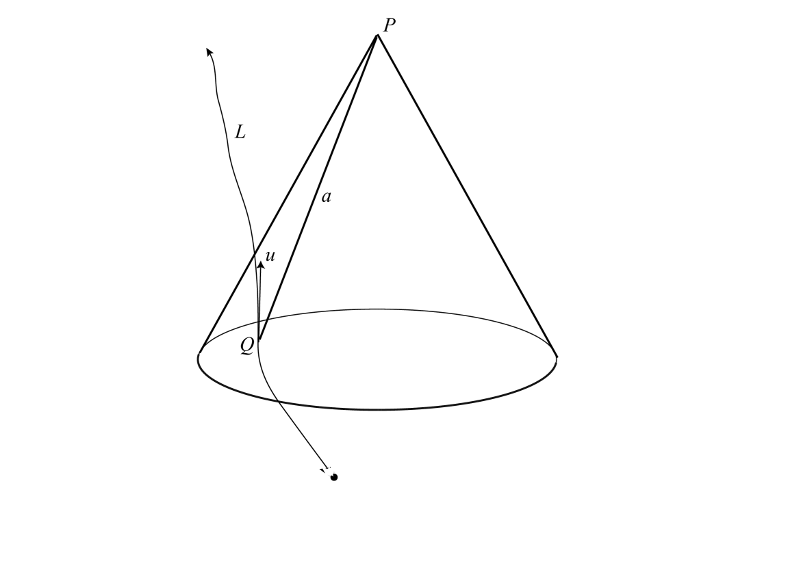
Figure 1: The four-vectors associated with an observer and a moving charge.

Let $K$ be an inertial reference frame in space-time with BT $\{\mathbf{n}_{\mu}\}.$ and coordinates $(y^{0},y^{1},y^{2},y^{3}).$ Denote by $y^{\mu}$ the coordinates of $P$ in this basis and denote by $\tilde{y}^{\mu}$ the the coordinates$Q$ of of the charge at the retarded time. Introduce a 4-vector $a=\overrightarrow{QP}$. Its coordinates in the BT are

$$a^{\mu}=y^{\mu}-\tilde{y}^{\mu}\,.$$ (35)

This vector is a null (light-like) vector in space-time and thus satisfies (8). Denote by $w=w(P)=w^{\nu}$ the 4-velocity of the charge at the point $P$ with coordinates expressed in BT, corresponding to time $\tilde{\tau}$. Note that only two 4-vectors: the null-vector $a$ defining the relative position of the charge at retarded time with respect to the point of observation of the potential, and the time-like vector $w$ of length 1 describing the 4-velocity of the charge at the retarded time, are independent of the choice of the reference frame.

From these two vectors we can generate a co-variant scalar $a\cdot w$. From the previous section, we know that there is also a dimension-less scalar $\zeta=\frac{a^{2}}{a^{0}}=\frac{a^{3}}{a^{1}}$ invariant under the representation $\tilde{\pi}$. We want the scalar potential to be a function of this dimension-less scalar.

To identify the function of the scalar potential, note that the electric force depends on the distance from the charge as $\frac{1}{r^{2}}$ and, as it was explained in the Introduction, the force has to be a second derivative of the potential. So, the natural candidate for the function of the scalar potential is a function proportional to $\ln$.

Definition We define a scalar complex potential $S(P)$ at the observer point $P$ of a moving charge $q$ by

$$S(P)=q\ln\zeta,$$ (36)

where $\zeta$ is the dimension-less scalar associated with the null vector $a=\overrightarrow{QP}$ connecting the position of the charge $Q$ at retarded time with the observer point. In BT this potential is equal

$$S(P)=q\ln\left(\frac{a^{2}}{a^{0}}\right)=q(\ln a^{2}-\ln a^{0})=q\ln\left(\frac{a^{3}}{a^{1}}\right)=q(\ln a^{3}-\ln a^{1}),$$ (37)

with $a^{\mu}$ defined by (35). For the usual basis, from (34) this potential is

$$S(P)=q\ln\zeta=q\ln\frac{x^{1}-ix^{2}}{x^{0}+x^{3}}=q\ln(\tan\frac{\theta}{2})-iq\varphi,$$ (38)

where $\varphi,\theta$, as in (33) are the angles in spherical coordinates of the space component of the vector $a=\overrightarrow{QP}$.

Our complex scalar potential $S$ is a combination $F-iG$ of the two scalar potentials introduced by Whittaker, see Whittaker and Ruse .

VIII The 4-potential and the electromagnetic field of a moving charge

For future calculations, we will need a formula for partial derivatives of $a$ and the retarded time $\tilde{\tau}$ with respect to $y^{\mu}$, for any given $\mu$. Denote by $\check{P}=P+\Delta^{\mu}P$ the point with coordinates $y+dy^{\mu}$ and by $\check{Q}=Q+\Delta^{\mu}Q$ the position of the charge at the corresponding retarded time. To first order in $dy^{\mu}$, we can write $\Delta^{\mu}Q=d\tilde{\tau}w^{\mu}$ for some $d\tilde{\tau}.$ Then the 4-vector $\check{a}=\overrightarrow{\check{Q}\check{P}}$ is approximately $\check{a}=a+dy^{\mu}-d\tilde{\tau}w^{\mu}$. Since $\check{a}$ and $a$ are null, we get, to first order,

$$(\check{a})^{2}=0\;\Rightarrow(a)^{2}-2\tilde{\eta}_{\lambda\nu}a^{\lambda}w^{\nu}d\tilde{\tau}+2\tilde{\eta}_{\mu\nu}a^{\nu}dy^{\mu}=0\;\Rightarrow\tilde{\eta}_{\mu\nu}a^{\nu}dy^{\mu}=(a\cdot w)d\tilde{\tau}.$$

Thus,

$$\frac{\partial\tilde{\tau}}{\partial y^{\mu}}=\frac{\tilde{\eta}_{\mu\nu}a^{\nu}}{a\cdot w}=\frac{a_{\mu}}{a\cdot w}.$$ (39)

From (35), the component $\nu$ of $a$ is $a^{\nu}=y^{\nu}-\tilde{y}^{\nu}$. Thus,

$$\frac{\partial a^{\nu}}{\partial y^{\mu}}=\delta_{\mu}^{\nu}-\frac{\partial\tilde{y}^{\nu}}{\partial y^{\mu}}=\delta_{\mu}^{\nu}-\frac{\partial\tilde{y}^{\nu}}{\partial\tilde{\tau}}\frac{\partial\tilde{\tau}}{\partial y^{\mu}}=\delta_{\mu}^{\nu}-\frac{w^{\nu}a_{\mu}}{a\cdot w}\,.$$ (40)

This gives

$$\frac{\partial(a\cdot w)^{-1}}{\partial y^{\mu}}=-(a\cdot w)^{-2}\frac{\partial(a\cdot w)}{\partial y^{\mu}}=-(a\cdot w)^{-2}\frac{\partial(\tilde{\eta}_{\lambda\nu}w^{\lambda}a^{\nu})}{\partial y^{\mu}}=-(a\cdot w)^{-2}\tilde{\eta}_{\lambda\nu}\left(a^{\nu}\frac{\partial w^{\lambda}}{\partial y^{\mu}}+w^{\lambda}\frac{\partial a^{\nu}}{\partial y^{\mu}}\right).$$

We assume now that $\frac{\partial w^{\lambda}}{\partial y^{\mu}}=0$, excluding accelerating charges. Then, by use of (40) and the fact that $(w)^{2}=\tilde{\eta}_{lk}w^{l}w^{k}=1$, we get

$$\frac{\partial(a\cdot w)^{-1}}{\partial y^{\mu}}=-(a\cdot w)^{-2}\tilde{\eta}_{\lambda\nu}w^{\lambda}(\delta_{\mu}^{\nu}-\frac{w^{\nu}a_{\mu}}{a\cdot w})=(a\cdot w)^{-2}(\frac{a_{\mu}}{a\cdot w}-w_{\mu})=\frac{a_{\mu}}{(a\cdot w)^{3}}-\frac{w_{\mu}}{(a\cdot w)^{2}}.$$ (41)

We define a complex 4-potential $\tilde{A}_{\mu}$ to be the conjugate to the gradient of the scalar complex potential vector. By use of (32) we have

$$\tilde{A}_{\mu}=-J_{\mu}^{\nu}\frac{\partial S}{\partial y^{\nu}}=-J_{\mu}^{\nu}\tilde{\partial}_{\nu}S=(-\frac{\partial S}{\partial y^{0}},-\frac{\partial S}{\partial y^{1}},\frac{\partial S}{\partial y^{2}},\frac{\partial S}{\partial y^{3}})\,.$$ (42)

Using (40), we get:

$$\tilde{A}_{0}=\frac{\partial S}{\partial y^{0}}=\frac{\partial q(\ln a^{3}-\ln a^{1})}{\partial y^{0}}=\frac{q}{a^{3}}\,\frac{w^{3}a_{0}}{a\cdot w}-\frac{q}{a^{1}}\,\frac{w^{1}a_{0}}{a\cdot w}=\frac{q}{a\cdot w}\left(w_{0}-a_{0}\frac{w^{1}}{a^{1}}\right),$$

$$\tilde{A}_{1}=\frac{\partial S}{\partial y^{1}}=\frac{\partial q(\ln a^{2}-\ln a^{0})}{\partial y^{1}}=\frac{q}{a^{2}}\,\frac{w^{2}a_{1}}{a\cdot w}-\frac{q}{a^{0}}\,\frac{w^{0}a_{1}}{a\cdot w}=\frac{q}{a\cdot w}\left(w_{1}-a_{1}\frac{w^{0}}{a^{0}}\right),$$

$$\tilde{A}_{2}=-\frac{\partial S}{\partial y^{2}}=\frac{\partial q(\ln a^{1}-\ln a^{3})}{\partial y^{2}}=\frac{q}{a^{1}}\,\frac{w^{1}a_{2}}{a\cdot w}-\frac{q}{a^{3}}\,\frac{w^{3}a_{2}}{a\cdot w}=\frac{q}{a\cdot w}\left(w_{2}-a_{2}\frac{w^{3}}{a^{3}}\right),$$

$$\tilde{A}_{3}=-\frac{\partial S}{\partial y^{3}}=\frac{\partial q(\ln a^{0}-\ln a^{2})}{\partial y^{3}}=\frac{q}{a^{0}}\,\frac{w^{0}a_{3}}{a\cdot w}-\frac{q}{a^{2}}\,\frac{w^{2}a_{3}}{a\cdot w}=\frac{q}{a\cdot w}\left(w_{3}-a_{3}\frac{w^{2}}{a^{2}}\right).$$

IX The electromagnetic field of a moving charge

By substituting (42) into (23) we get

$$F_{j}=-\tilde{\partial}^{\nu}(I_{2}\otimes\sigma_{j})^{\mu}_{\nu}\tilde{A}_{\mu}=\tilde{\partial}^{\nu}(I_{2}\otimes\sigma_{j})^{\mu}_{\nu}J_{\mu}^{\lambda}\tilde{\partial}_{\lambda}S.$$

Since

$$(I_{2}\otimes\sigma_{j})^{\mu}_{\nu}J_{\mu}^{\lambda}=\left(\begin{array}[]{cc}\sigma_{j}&0\\ 0&-\sigma_{j}\\ \end{array}\right)=(\alpha_{j})_{\nu}^{\lambda}\,,$$

where $(\alpha_{j})$ are the known $\alpha$-matrices of Dirac, (see LL4 ) we have:

$$F_{j}=\tilde{\partial}^{\nu}(\alpha_{j})_{\nu}^{\lambda}\tilde{\partial}_{\lambda}S.$$ (43)

This give explicit formulas for each component of the $F$:

$$F_{1}=\frac{\partial^{2}S}{\partial y^{1}\partial y^{3}}-\frac{\partial^{2}S}{\partial y^{0}\partial y^{2}},\;\;F_{2}=i\left(\frac{\partial^{2}S}{\partial y^{1}\partial y^{3}}+\frac{\partial^{2}S}{\partial y^{0}\partial y^{2}}\right)\,,$$

$$F_{3}=\frac{\partial^{2}S}{\partial y^{1}\partial y^{2}}+\frac{\partial^{2}S}{\partial y^{0}\partial y^{3}}\,.$$

By differentiating the first derivatives of $S$ and applying (40) and (41), for the potential of a moving charge we get

$$\frac{\partial^{2}S}{\partial y^{1}\partial y^{3}}=q\frac{w^{0}a_{1}+w^{2}a_{3}}{(a\cdot w)^{3}},\;\;\;\;\frac{\partial^{2}S}{\partial y^{0}\partial y^{2}}=-q\frac{w^{1}a_{0}+w^{3}a_{2}}{(a\cdot w)^{3}},$$

and

$$\frac{\partial^{2}S}{\partial y^{1}\partial y^{2}}=\frac{q}{2(a\cdot w)^{2}}-q\frac{w^{3}a_{3}+w^{1}a_{1}}{(a\cdot w)^{3}}$$

$$\frac{\partial^{2}S}{\partial y^{0}\partial y^{3}}=\frac{-q}{2(a\cdot w)^{2}}+q\frac{w^{0}a_{0}+w^{2}a_{2}}{(a\cdot w)^{3}}\,.$$

This defines a formula for the Faraday vector of the electromagnetic field of a moving charge

$$F_{j}=q\frac{a_{\mu}(\tilde{K}_{j})_{\nu}^{\mu}w^{\nu}}{(a\cdot w)^{3}}\,,$$ (44)

where $(\tilde{K}_{j})_{\nu}^{\mu}$ is defined by (22).

In the basis $\mathbf{e}_{\mu}$ this formula becomes

$$F_{j}=q\frac{x_{0}u_{j}-x_{j}u_{0}+i\varepsilon_{j}^{kl}(x_{k}u_{l})}{(x\cdot u)^{3}}\,,$$ (45)

This formula coincides with the usual formula for the field of a moving charge (see, for example, Jackson p. 573 ).

Direct calculation shows that $S$ satisfies the wave equation

$$\square^{2}S=\tilde{\partial}^{\mu}\tilde{\partial}_{\mu}=2\left(\frac{\partial^{2}S}{\partial y^{0}\partial y^{3}}-\frac{\partial^{2}S}{\partial y^{1}\partial y^{2}}\right)=0\,.$$ (46)

For the 4-potential (42) this implies that

$$\frac{\partial\tilde{A}_{3}}{\partial y^{0}}-\frac{\partial\tilde{A}_{1}}{\partial y^{2}}=0,\;\;\frac{\partial\tilde{A}_{0}}{\partial y^{3}}-\frac{\partial\tilde{A}_{2}}{\partial y^{1}}=0\,.$$ (47)

X Scalar complex potential of an electromagnetic field

Any electromagnetic field is generated by a collection of moving charges. We may assume that charges close to each other move with velocities that do not vary significantly. The sources of the electromagnetic field may be represented by the charge densities $\rho(x)$ on space-time 4-vector $x$. We assume that the potential depends additively on the charges generating the field. By choosing a BT in space-time, the scalar complex potential of the electromagnetic field is given by

$$S(y)=\int_{S^{-}(y)}\ln(\frac{a^{2}}{a^{0}})\rho(y+a)da,$$ (48)

where $S^{-}(y)$ denotes the backward light-cone at $y$.

Let us return back to the usual basis $\{\mathbf{e}_{\mu}\}$ in space-time. If we use spherical coordinates in space as in (33) and the formula (38) for the scalar potential of a charge, then we can rewrite (48) as

$$S(x)=\int_{0}^{2\pi}d\varphi\int_{0}^{\pi}\ln(\tan\frac{\theta}{2})\sin\theta d\theta\int_{0}^{\infty}\rho(x+r\,n(\varphi,\theta))r^{2}dr-i\int_{0}^{2\pi}\varphi d\varphi\int_{0}^{\pi}\sin\theta d\theta\int_{0}^{\infty}\rho(x+r\,n(\varphi,\theta))r^{2}dr\;.$$ (49)

Since equation (46) is a linear homogeneous equation it will hold for for a scalar potential of arbitrary electromagnetic field. Also equations (47) will hold for such a field. Using these equations and (25) we get obtain the following formula for the connection of the 4-potential and Faraday tensor

$$\widetilde{\mathcal{F}}_{\alpha\beta}=\left(\begin{array}[]{cc}0&1\\ -1&0\\ \end{array}\right)\otimes\left(\begin{array}[]{cc}\left(\frac{\partial\tilde{A}_{0}}{\partial y^{2}}-\frac{\partial\tilde{A}_{2}}{\partial y^{0}}\right)&\left(\frac{\partial\tilde{A}_{3}}{\partial y^{0}}-\frac{\partial\tilde{A}_{0}}{\partial y^{3}}\right)\\ \left(\frac{\partial\tilde{A}_{2}}{\partial y^{1}}-\frac{\partial\tilde{A}_{1}}{\partial y^{2}}\right)&\left(\frac{\partial\tilde{A}_{1}}{\partial y^{3}}-\frac{\partial\tilde{A}_{3}}{\partial y^{1}}\right)\\ \end{array}\right)=(-1)^{(\alpha+\beta)}\left(\frac{\partial\tilde{A}_{\alpha}}{\partial y^{\beta}}-\frac{\partial\tilde{A}_{\beta}}{\partial y^{\alpha}}\right)\,.$$ (50)

This show that our differential operator $\widetilde{\nabla}_{c}\times$ in (25) is

$$(\widetilde{\nabla}_{c}\times)^{\mu}_{\alpha\beta}=(-1)^{(\alpha+\beta)}\left(\delta^{\mu}_{\alpha}\partial_{\beta}-\delta^{\mu}_{\beta}\partial_{\alpha}\right),$$ (51)

which is close to the $curl=({\nabla}\times)^{\mu}_{\alpha\beta}=\delta^{\mu}_{\alpha}\partial_{\beta}-\delta^{\mu}_{\beta}\partial_{\alpha}$. Note that without conjugation in definition of $\tilde{A}^{\mu}$, we would get a zero answer for $\widetilde{\mathcal{F}}_{\alpha\beta}$. This corresponds to the known identity $\nabla\times\nabla S=0$ for any scalar function $S$.

XI Discussion and conclusion

We have shown that the E. T. Whittaker scalar potentials of a moving charge became one complex potential (38)on space-time. Thus, any electromagnetic field can be described by use of the complex scalar potential which is as the wave-function of Quantum Mechanics, a complex-valued function on space-time. We defined a representation $\tilde{\pi}$ of the Lorentz group on the complexified Minkowski space $M$ and its adjoint one $\tilde{\pi}^{*}$, which commutes with it. The usual representation $\pi$ of the Lorentz group on $M$ is the product of representations $\tilde{\pi}$ and $\tilde{\pi}^{*}$. We defined a Lorentz Invariant conjugation (32) on $M$ under the representation $\tilde{\pi}$.

For any electromagnetic field by use of (49) we obtain a complex-valued function, that we called the complex scalar potential, which is defined by the distribution of the charges generating the field. The components of the Faraday vector, describing the electro-magnetic force of the field, may be obtained from the potential by (43) as

$$F_{j}=\tilde{\partial}^{\nu}(\alpha_{j})_{\nu}^{\lambda}\tilde{\partial}_{\lambda}S.$$

where $(\alpha_{j})$ are the known $\alpha$-matrices of Dirac. This ones more reveals the connection between our description of the classical electromagnetic field and Quantum Mechanics. From the Claim in Section 6, it follows that the complex scalar potential is an invariant scalar under the representation $\tilde{\pi}$.

We show that the Faraday tensor $\widetilde{\mathcal{F}}$ is the complexified $curl$ defined by (51) of the conjugate of the gradient of the complex potential, which can be written as.

$$\widetilde{\mathcal{F}}=\widetilde{\nabla}_{c}\times(\widetilde{\nabla}S)^{\#}\,.$$ (52)

The real part of the Faraday tensor $\mathcal{F}$ coincides with the usual electromagnetic tensor of the field. We obtain an explicit formula for the Faraday vector (45) of a moving charge. We have shown that the complex scalar potential satisfies the wave equation (46).

Note that the complex logarithm is not defined uniquely. So,the scalar complex potential is a multi-valued function. The Aharonov-Bohm effect AharonovBohm59 revealed that in presence of an electromagnetic field the wave function of a particle is multiplied by a multi-valued function defined by the field. This is similar to our observation.

The first author would like to thank Prof. Donald Lynden-Bell for bringing to his attention the result of E. T. Whittaker and providing him with a copy of Whittaker’s paper. Both would like to thank Prof. U. Sandler, Dr. Y. Itin, Dr. V. Ostapenko and Dr. Z. Scaar for helpful discussions and remarks.

References

(1) Aharonov, Y., and Bohm, D,
Significance of Electromagnetic Potential in Quantum Theory,
Phys. Rev.115, No. 3 (1959); pp. 485-491
(2)Barut A. O., Electrodynamicsand Classical Theory of Fields & Particles Dover Publ.
NY, 1980.
(3) Baylis W. E., Electrodynamics, A Modern Geometric Approach, Progress in
Physics 17, Birkhäuser, Boston, 1999.
(4) Friedman, Y., “Representations of the Poincaré group on relativistic phase
space”, arXiv:0802.0070v1, 2008.
(5) Friedman, Y., “The relativistic phase space and Newman-Penrose basis”,
arXiv:0901.1040v1, 2009.
(6)Y. Friedman, Physical Applications of Homogeneous Balls,
Progress in Mathematical Physics 40, Birkhäuser,
Boston, (2004).
(7) Y. Friedman, M. Danziger, “The complex Faraday tensor for relativistic
evolution of a charged particle in a constant field”, PIERS 2008,
Cambridge
(8) Friedman, Y. and Semon M., “Relativistic acceleration of charged particles in
uniform and mutually perpendicular electric and magnetic fields as viewed in
the laboratory frame” , Phys. Rev. E Vol. 72, No. 2, 026603 2005.
(9) Jackson, J. D., Classical Electrodynamics, Wiley & Sons, New York, 1999.
(10) Jeans J. H., Mathematical theory of Electricity and
Magnetism, Cambridge, 575, 1923.
(11) P. O’Donnell, Introduction to 2-Spinors in
General Relativity, World Scientific Pub., 2003.
(12) R. Penrose & W. Rindler, Spinors and
space-time, Cabridge University Press, 1984.
(13) Muñoz, G. “Charged Particle in a Constant Electromagnetic Field: Covariant Solution”, American Journal of Physics, Vol. 65, No. 5 429–433, 1997.
(14) Landau, L.D. and Lifschitz E.M., The Classical Theory of Fields, Pergamon, Oxford, 1962.
(16) Ruse H. S. “ On Whittaker’s electomagnetic scalar
potetials” (1937).
(17) Silberstein L., “Nachtrag zur Abhandlung über Electromagnetische Grundgleichungen in bivektorieller
Behandlung”, Ann. Phys. Lpz.24, 783–784 (1907).
(18) Silberstein L., The Theory of Relativity Macmillan and Co., London, 1927.
(19) Whittaker E. T., “ On an expression of the
electromagnetic field due to electrons by means of two scalar
potential functions”, Proc. London Math. Soc.,
2, 367–372, 1904.