Quantum mechanics in phase space:
First order comparison between the Wigner and the Fermi function

Abstract

The Fermi $g_{F}(x,p)$ function provides a phase space description of quantum mechanics conceptually different from that based on the the Wigner function $W(x,p)$. In this paper, we show that for a peaked wave packet the $g_{F}(x,p)=0$ curve approximately corresponds to a phase space contour level of the Wigner function and provides a satisfactory description of the wave packet’s size and shape. Our results show that the Fermi function is an interesting tool to investigate quantum fluctuations in the semiclassical regime.

I Introduction

The Wigner phase space representation of quantum mechanics wigner ; wignerreview ; zachos is a very useful and enlightening approach. It is of practical interest in the description of a broad range of physical phenomena, including quantum transport processes in quantum optics schleich and condensed matter jacoboni , quantum chaos saraceno , quantum complexity benenti , decoherence zurek , quantum computation saraceno2 ; terraneo , and quantum tomography wootters . Furthermore, the phase space approach brings out most clearly the differences and similarities between classical and quantum mechanics and offers unique insights into the classical limit of quantum theory heller ; berry ; brumer ; davidovich ; habib .

The Wigner phase space distribution function of a quantum state described by a state vector $|\psi\rangle$ reads

$$W(x,p)\equiv\frac{1}{2\pi\hbar}\int_{-\infty}^{\infty}dye^{-\frac{i}{\hbar}py}\psi\left(x+\frac{y}{2}\right)\psi^{\star}\left(x-\frac{y}{2}\right).$$ (1)

(For the sake of simplicity, we consider the case of a single particle moving along a straight line). The Wigner function provides a pictorial phase-space representation of the abstract notion of a quantum state and allows us to compute the quantum mechanical expectation values of observables in terms of phase space-averages.

A different, almost unknown phase space approach is based on an old paper by Fermi fermi . As pointed out by Fermi, the state of a quantum system may be defined in two completely equivalent ways: by its wave function $\psi(x)=\langle x|\psi\rangle$ or by measuring a physical quantity $g_{F}(x,p)$. Given the measurement outcome $g_{F}(x,p)=\bar{g}$, $\psi(x)$ is obtained as solution of the eigenvalue equation $g_{F}(x,p)\psi(x)=\bar{g}\psi(x)$, where $p=-i\hbar{\partial_{x}}$. On the other hand, given the wave function $\psi(x)$ it is always possible to find an operator $g_{F}(x,p)$ such that

$$g_{F}(x,p)\psi(x)=0.$$ (2)

Using the polar decomposition

$$\psi(x)=R(x)e^{\frac{i}{\hbar}S(x)},$$ (3)

where $R(x)$ and $S(x)$ are real functions [$R(x)\geq 0$ for any $x$], it is easy to check that identity (2) is fulfilled by taking

$${g}_{F}\left(x,-i\hbar\partial_{x}\right)=\left[-i\hbar\partial_{x}-S^{\prime}(x)\right]^{2}+\hbar^{2}\frac{R^{\prime\prime}(x)}{R(x)}.$$ (4)

Equation (2) implies that the corresponding physical quantity $g_{F}(x,p)$ takes the value $\bar{g}=0$. The equation

$$g_{F}(x,p)=\left[p-S^{\prime}(x)\right]^{2}+\hbar^{2}\frac{R^{\prime\prime}(x)}{R(x)}=0$$ (5)

defines a curve in the two-dimensional phase space. In other words, as expected from Heisenberg uncertainty principle, we cannot identify a quantum particle by means of a phase-space point $(x,p)$ but we need a curve, $g_{F}(x,p)=0$. Note that it is also possible to write equation (5) in the form

$$p_{\pm}=S^{\prime}(x)\pm\sqrt{-\hbar^{2}\frac{R^{\prime\prime}(x)}{R(x)}}=mv_{M}\pm\sqrt{2mV_{Q}},$$ (6)

where $m$ is the particle mass, $v_{M}\equiv\frac{1}{m}S^{\prime}$ the Madelung’s velocity  madelung , and $V_{Q}\equiv-\frac{\hbar^{2}}{2m}\frac{R^{\prime\prime}}{R}$ the so-called quantum-mechanical potential bohm . Equation (6) locates two points, $(x,p_{+})$ and $(x,p_{-})$, in the phase space for any $x$ such that $R^{\prime\prime}(x)<0$ and $R(x)\neq 0$.

The phase space Fermi function $g_{F}(x,p)$ and the Wigner function $W(x,p)$ are at first sight unrelated. In particular, for the Fermi function there is no interpretation in terms of quasiprobabilities as for the Wigner function. On the other hand, for a Gaussian wave packet the $g_{F}(x,p)=0$ curve is an ellipse of area $\pi\hbar$ strini1 ; strini2 and coincides with the phase-space contour level along which $W(x,p)=W_{\rm max}/e$, with $W_{\rm max}$ equal to the maximum value of $W$. Different contour levels of $W$ correspond to different “equipotential curves” $g_{F}={\rm constant}$. The purpose of the present paper is to show that a similar relation exists when the Gaussian shape of the wave packet is modified, provided the wave packet remains peaked. Finally, we will comment on the significance of our results in the context of semiclassical approximations of quantum mechanics.

II Gaussian packets

Let us first consider the Gaussian packet

$$R(x)=G(x)\equiv\frac{1}{\sqrt{\sqrt{\pi}\delta}}e^{-\frac{(x-x_{0})^{2}}{2\delta^{2}}},\;\;S(x)=p_{0}x.$$ (7)

In this case Wigner function (1) reads

$$W(x,p)=\frac{1}{\pi\hbar}e^{-\frac{(x-x_{0})^{2}}{\delta^{2}}-\frac{\delta^{2}(p-p_{0})^{2}}{\hbar^{2}}},$$ (8)

while the Fermi function is given by

$$g_{F}(x,p)=\frac{\hbar^{2}(x-x_{0})^{2}}{\delta^{4}}+(p-p_{0})^{2}-\frac{\hbar^{2}}{\delta^{2}}.$$ (9)

It is clear from Eqs. (8) and (9) that for Gaussian packet (7) we have

$$W(x,p)=\frac{1}{\pi e\hbar}e^{-\frac{\delta^{2}}{\hbar^{2}}g_{F}(x,p)}.$$ (10)

Therefore, there is a one to one correspondence between the “equipotential curves” $g_{F}(x,p)=K$ and $W(x,p)=C$, with $C=\frac{1}{\pi e\hbar}e^{-\frac{\delta^{2}}{\hbar^{2}}K}$. In particular, the $g_{F}=0$ curve coincides with the curve $W=\frac{1}{\pi e\hbar}=\frac{W_{\rm max}}{e}$, with $W_{\rm max}=W(x_{0},p_{0})$ maximum value of $W$.

III Non-Gaussian packets

We now discuss the relation between the Wigner and the Fermi function when the wave packet is peaked but not Gaussian. Assuming a smooth, regular behavior of the packet around its maximum, we choose the analytic expression $R(x)=CG(x)[1+P(x)]$, with $P(x)$ polynomial [chosen so that $R(x)\geq 0$ for any $x$] and $C$ normalization constant which is irrelevant for our purposes, while $S(x)$ is a polynomial. The Wigner function is then given by the Fourier transform (1) of

$$\begin{array}[]{c}\psi\left(x+\frac{y}{2}\right)\psi^{\star}\left(x-\frac{y}{2}\right)=C^{2}G\left(x+\frac{y}{2}\right)G\left(x-\frac{y}{2}\right)\\ \\ \times\left[1+P\left(x+\frac{y}{2}\right)+P\left(x-\frac{y}{2}\right)+P\left(x+\frac{y}{2}\right)P\left(x-\frac{y}{2}\right)\right]\\ \\ \times\,e^{\frac{i}{\hbar}\left[S\left(x+\frac{y}{2}\right)-S\left(x-\frac{y}{2}\right)\right]}.\end{array}$$ (11)

III.1 Gaussian $R$

We computed numerically $W(x,p)$ for several functions $P(x)$, $S(x)$ and found that it strongly depends on $S(x)$, while the dependence on $P(x)$ is weak, as far as the wave packet remains peaked. Therefore, we first focus on the case $R(x)=G(x)$.

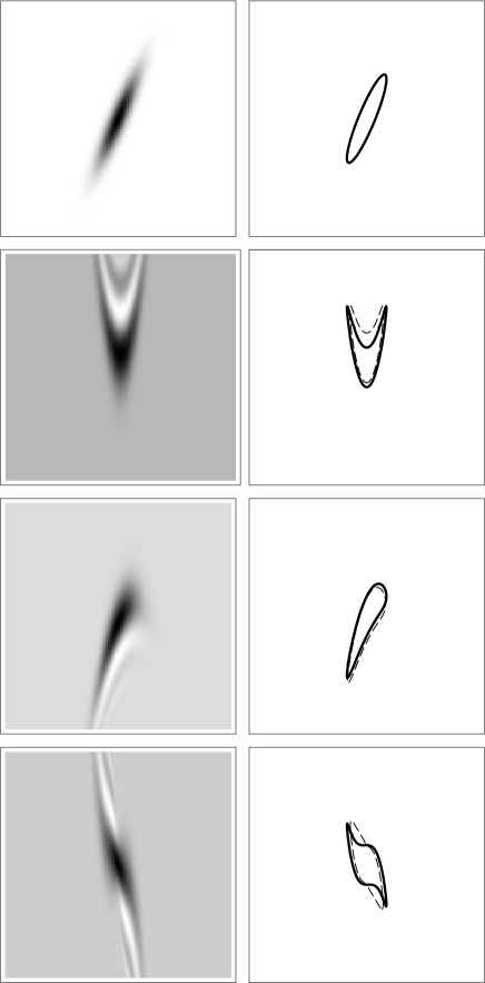
Figure 1: Plots of the Wigner function (left) and of the $g_{F}=0$ curve (right, thick full curves) for $R$ Gaussian and various $S$. Horizontal axis: $-6\leq\tilde{x}\leq 6$, with $\tilde{x}\equiv\frac{1}{\delta}(x-x_{0})$. Vertical axis: $-6\leq\tilde{p}\leq 6$, with $\tilde{p}\equiv\frac{\delta}{\hbar}(p-p_{0})$. From top to bottom: $\hbar S=\tilde{x}^{2}$, $\tilde{x}^{3}$, $\tilde{x}^{2}-\frac{1}{3}\tilde{x}^{3}$, and $-\frac{1}{2}\tilde{x}^{4}$. The thin dashed curves in the right plots correspond to the contour level $W=\frac{W_{\rm max}}{e}$ of the Wigner function. Note that for the top plot such contour level exactly coincide with the $g_{F}=0$ curve.

Wigner functions for $P(x)=0$, namely

$$\psi(x)=G(x)e^{\frac{i}{\hbar}S(x)},$$ (12)

and several $S(x)$ are shown in Fig. 1 (left plot) and compared with the corresponding $g_{F}=0$ curves (right plots). Even though the wave packets in Fig. 1, with the exception of the top plot [$S(x)\propto x^{2}$, corresponding to a squeezed state], are far from being Gaussian, the $g_{F}=0$ curve still provides a rather satisfactory description of size and shape of the wave packet in phase space.

This agreement can be explained by the following argument. If we set $P(x)=0$ and consider the expansion

$$\begin{array}[]{c}S\left(x+\frac{y}{2}\right)-S\left(x-\frac{y}{2}\right)\\ \\ =S^{\prime}(x)y+\frac{1}{24}S^{\prime\prime\prime}(x)y^{3}+O(y^{5})\approx S^{\prime}(x)y,\end{array}$$ (13)

we obtain

$$\psi\left(x+\frac{y}{2}\right)\psi^{\star}\left(x-\frac{y}{2}\right)\approx F(x,y)e^{\frac{i}{\hbar}S^{\prime}(x)y},$$ (14)

where $F(x,y)\equiv G\left(x+\frac{y}{2}\right)G\left(x-\frac{y}{2}\right)$. Therefore, the shift theorem of Fourier transform implies that, if

$${\cal F}_{y}[F(x,y)]=W_{G}(x,p),$$ (15)

with ${\cal F}_{y}$ Fourier transform with respect to the $y$-variable, then

$${\cal F}_{y}\left[F(x,y)e^{\frac{i}{\hbar}S^{\prime}(x)y}\right]=W_{G}[x,p-S^{\prime}(x)].$$ (16)

We can therefore conclude that the Wigner function corresponding to wave vector (12) reads

$$W(x,p)\approx W_{G}[x,p-S^{\prime}(x)]=\frac{1}{\pi\hbar}e^{-\frac{(x-x_{0})^{2}}{\delta^{2}}-\frac{\delta^{2}[p-S^{\prime}(x)]^{2}}{\hbar^{2}}}.$$ (17)

Hence connection (10) between the Wigner and the Fermi functions approximately holds around the peak of the wave packet. The rather good agreement between the $g_{F}=0$ curve and the contour level $W=\frac{W_{\rm max}}{e}$ is shown in the right plots of Fig. 1. We can conclude that, for peaked packets, the $g_{F}=0$ curve is close to an equipotential curve of the Wigner function, enclosing a phase space area of the order of Planck’s constant.

III.2 Non-Gaussian $R$, $S=0$

We have seen numerically that the dependence of the Wigner function on $P(x)$ is weak, as far as the wave packet remains peaked. As an example, we consider $P(x)=1+a\frac{(x-x_{0})^{2}}{\delta^{2}}$, with $a>0$ so that $R(x)>0$ for any $x$, and $S=0$. For $a<\frac{1}{2}$ the wave function $\psi(x)=R(x)$ has a single maximum at $x=0$ and the $g_{F}=0$ curve again gives a good representation of the phase-space size and shape of the wave packet (see the top plots of Fig. 2). On the other hand, for $a>\frac{1}{2}$ the wave function exhibits two maxima at $x_{\pm}=\pm\delta\sqrt{2-\frac{1}{a}}$. For $a\gg 1$ the two maxima are well separated. Such a ”cat state” exhibits non-classical features which impact on the structure of the Wigner function (see Fig. 2 bottom left, for $a=10$). Since $W(x,p=0)$ is the autocorrelation function of $R(x)$, then it reaches its maximum at $x=0$. On the other hand, the marginal $\int dpW(x,p)=|\psi(x)|^{2}=R^{2}(x)$ exhibits a minimum at $x=0$ and this is possible thanks to the negative regions of $W(x,p)$ (the white regions in Fig. 2 bottom left). For this cat state the $g_{F}=0$ curve captures the two peaks at $x_{\pm}$ (see Fig. 2 bottom right) but not the non-classical phase-space structures of the Wigner function.

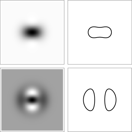
Figure 2: Plots of the Wigner function (left) and of the $g_{F}=0$ curve (right, thick full curves) for $P=1+a\tilde{x}^{2}$, $a=0.3$ (top) and $a=10$ (bottom), and $S=0$. Horizontal axis: $-4\leq\tilde{x}\leq 4$. Vertical axis: $-4\leq\tilde{p}\leq 4$.

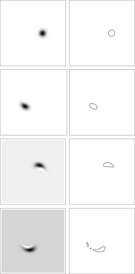
Figure 3: Plots of the Wigner function (left) and of the $g_{F}=0$ curve (right) for the quartic oscillator, with $\hbar\lambda/\omega=0.01$. Horizontal axis: $-10\leq\tilde{x}\leq 10$, with $\tilde{x}\equiv\sqrt{\frac{m\omega}{\hbar}}x$. Vertical axis: $-10\leq\tilde{p}\leq 10$, with $\tilde{p}\equiv\sqrt{\frac{1}{\hbar m\omega}}p$. From top to bottom: $t/T=0,0.4,0.8,1.2$, with $T=2\pi/\omega$. The initial Gaussian distribution is centered in $(\tilde{x},\tilde{p})=(3,0)$.

IV A dynamical example: the quartic oscillator

The $g_{F}=0$ curve is an interesting tool to investigate quantum fluctuations in the semiclassical region. As far as the wave packet remains peaked, that is, before the Ehrenfest time scale berman , its size and phase-space shape can be readily derived from the wave function (or from a semiclassical approximation of the wave function), without computing the whole Wigner function. Moreover, the distortion of the wave packet is directly related to $S^{\prime}(x)$, that is, to the Madelung’s velocity.

As a numerical illustration of the capability of the $g_{F}=0$ curve to capture relevant features of quantum fluctuations, we follow in Fig. 3 the evolution of the Wigner and Fermi functions for the quartic oscillator Hamiltonian

$$H=\hbar\omega a^{\dagger}a+\hbar^{2}\lambda(a^{\dagger})^{2}a^{2}.$$ (18)

Here, $a=\sqrt{\frac{1}{\hbar m\omega}}(m\omega x+ip)$, $\omega$ is the frequency of the harmonic part of the oscillator and $\hbar\lambda$ gives the strength of the nonlinearity. This model has been widely investigated in the context of quantum to classical transition berman ; milburn ; angelo ; oliveira and also used to explain important experimental results bloch . Model (18) is integrable, see Refs. milburn ; oliveira for the evolution of classical and quantum phase-space distributions. Details on the computation of the Fermi function are given in the Appendix.

In Fig. 3 we compare the evolution the Wigner function with the evolution of the $g_{F}=0$ Fermi function, for the quartic oscillator, starting from an initial Gaussian wave packet $|\alpha\rangle$ ($a|\alpha\rangle=\alpha|\alpha\rangle$). It is clear that, as far as the wave packet remains peaked, the $g_{F}=0$ curve reproduces both size and shape of quantum fluctuations. This is the case for times smaller than the Ehrenfest time scale $t_{E}\sim\frac{1}{\hbar\lambda|\alpha|}$ berman , until which the centroid of the wave packet follows a classical trajectory. For longer times the Wigner function develops interference fringes, while the $g_{F}=0$ function splits into several curves. We point out that the $g_{F}(x,p)=0$ function (6) singles out only two $p$-values (or none) for any $q$. Therefore, it cannot reproduce the whole phase space structure of the wave packet when the Wigner function does not exhibit a single peak but a non-monotonous behavior along $p$ [see the bottom plot of Fig. 3 (left)].

V Concluding remarks

In summary, we have shown that the phase space structure of a peaked wave packet can be satisfactorily described by the $g_{F}=0$ Fermi curve. In spite of the fact that the Wigner and the Fermi functions are at first sight two completely unrelated phase space descriptions of quantum mechanics, a link between them exists and is based on the shift theorem of Fourier transform. Such theorem also allows us to understand the shape of the Wigner function for perturbed Gaussian packets in terms of the Madelung’s velocity. Our theoretical results, corroborated by numerical simulations for the quartic oscillator model, show that the Fermi function is an interesting tool to investigate the phase-space size and shape of quantum fluctuations in the semiclassical regime.

While the Fermi function $g_{F}(x,p)$ fully determines the state of a quantum system, the extension of the results obtained in this paper to generic states encounters difficulties. Knowledge of the $g_{F}(x,p)=0$ curve is in general not sufficient. The complete determination of the state of a system requires the extension of this curve to the complex $p$-plane. That is, consideration of the complex values of $p_{\pm}$, obtained from Eq. (6) when $R^{\prime\prime}>0$, is needed. We then obtain $S^{\prime}=\frac{p_{+}+p_{-}}{2}$, $\hbar^{2}\frac{R^{\prime\prime}}{R}=-\left(\frac{p_{+}-p_{-}}{2}\right)^{2}$, from which the $g_{F}$ operator (4) and consequently the wave function $\psi(x)$ are determined. Any phase space description of quantum mechanics necessarily involves features beyond classical intuition: negative quasiprobabilities in the case of the Wigner function, complex momenta for the Fermi curve.

Appendix A Fermi function for the quartic oscillator

We consider as initial condition a Gaussian state (coherent state for the harmonic part of the oscillator), $|\alpha\rangle=\sum_{n=0}^{\infty}c_{n}|n\rangle$, with $c_{n}=e^{-\frac{1}{2}|\alpha|^{2}}\frac{\alpha^{n}}{\sqrt{n!}}$, $a|\alpha\rangle=\alpha|\alpha\rangle$, $H|n\rangle=E_{n}|n\rangle$, $E_{n}=\hbar\omega+\hbar^{2}\lambda n(n-1)$. The state of the quartic oscillator at time $t$ is then given by $|\psi(t)\rangle=\sum_{n=0}^{\infty}c_{n}e^{-\frac{i}{\hbar}E_{n}t}|n\rangle$. In the coordinate representation,

$$\begin{array}[]{c}\phi_{n}(x)\equiv\langle x|n\rangle\\ \\ =\left(\frac{m\omega}{\pi\hbar}\right)^{1/4}\frac{1}{2^{n/2}\sqrt{n!}}H_{n}\left(\sqrt{\frac{m\omega}{\hbar}}x\right)e^{-\frac{1}{2}\frac{m\omega}{\hbar}x^{2}},\end{array}$$ (19)

where $H_{n}$ denotes the $n$-th Hermite polynomial.

In order to compute the Fermi function, we write $\psi=\psi_{R}+i\psi_{I}$, so that

$$\begin{array}[]{c}\frac{R^{\prime\prime}}{R}=\frac{1}{(\psi_{R}^{2}+\psi_{I}^{2})^{2}}(\psi_{R}\psi_{R}^{\prime}+\psi_{I}\psi_{I}^{\prime})^{2}\\ \\ +\frac{1}{\psi_{R}^{2}+\psi_{I}^{2}}\left[(\psi_{R}^{\prime})^{2}+(\psi_{I}^{\prime})^{2}+\psi_{R}\psi_{R}^{\prime\prime}+\psi_{I}\psi_{I}^{\prime\prime}\right],\end{array}$$ (20)

$$S^{\prime}=\frac{\psi_{R}\psi_{I}^{\prime}-\psi_{R}^{\prime}\psi_{I}}{\psi_{R}^{2}+\psi_{I}^{2}}.$$ (21)

Finally, the $g_{F}=0$ curve is obtained from (5). Note that in computing the derivatives of $\psi_{R}$ and $\psi_{I}$, we took advantage of the relation $H_{n}^{\prime}=2nH_{n-1}$. This property of Hermite polynomials allowed us to avoid numerical errors in the computation of the derivatives $R^{\prime\prime}$ and $S^{\prime}$.

References

- (1) E. Wigner, Phys. Rev. 40, 749 (1932).
- (2) M. Hillery, R.F. O’Connell, M.O. Scully, and E.P. Wigner, Phys. Rep 106, 121 (1984).
- (3) C. K. Zachos, D. B. Fairlie, and T. L. Curtright (Eds.), Quantum mechanics in phase space (World Scientific, Singapore, 2005).
- (4) W. P. Schleich, Quantum optics in phase space (Wiley-VCH Verlag, Berlin, 2001).
- (5) C. Jacoboni and P. Bordone, Rep. Prog. Phys. 67, 1033 (2004).
- (6) M. Saraceno, Ann. Phys. (NY) 199, 37 (1990).
- (7) G. Benenti and G. Casati, Phys. Rev. E 79, 025201(R) (2009).
- (8) W.H. Zurek, Rev. Mod. Phys. 75, 715 (2003).
- (9) C. Miquel, J. P. Paz, and M. Saraceno, Phys. Rev. A 65, 062309 (2002).
- (10) M. Terraneo, B. Georgeot, and D. L. Shepelyansky, Phys. Rev. E 71, 066215 (2005).
- (11) K. S. Gibbons, M. J. Hoffman, and W. K. Wootters, Phys. Rev. A 70, 062101 (2004).
- (12) E.J. Heller, J. Chem. Phys. 65, 1289 (1976).
- (13) M. V. Berry and N. L. Balazs, J. Phys. A 12, 625 (1979).
- (14) J. Gong and P. Brumer, Phys. Rev. A 68, 062103 (2003).
- (15) A.R.R. Carvalho, R.L. de Matos Filho, and L. Davidovich, Phys. Rev. E 70, 026211 (2004).
- (16) B.D. Greenbaum, S. Habib, K. Shizume, and B. Sundaram, Phys. Rev. E 76, 046215 (2007).
- (17) E. Fermi, Rend. Lincei 11, 980 (1930), reprinted in Nuovo Cimento 7, 361 (1930) [An english translation of Fermi’s paper is available upon request to giuliano.strini@mi.infn.it].
- (18) E. Madelung, Z. Phys. 40, 332 (1926).
- (19) D. Bohm, Phys. Rev. 85, 166 (1952).
- (20) A. M. Grassi and G. Strini, in R. Bonifacio (Ed.), Mysteries, puzzles, and paradoxes in quantum mechanics, AIP Conference Proceedings 461, 287 (1999).
- (21) G. Benenti and G. Strini, Am. J. Phys. 77, 546 (2009).
- (22) G. P. Berman and G. M. Zaslavsky, Physica A 91, 450 (1978); G. M. Zaslavsky, Phys. Rep. 80, 157 (1981).
- (23) G. J. Milburn, Phys. Rev. A 33, 674 (1986).
- (24) R. M. Angelo, L. Sanz, and K. Furuya, Phys. Rev. E 68, 016206 (2003).
- (25) A. C. Oliveira, M. C. Nemes, and K. M. Fonseca Romero, Phys. Rev. E 68, 036214 (2003); A. C. Oliveira, J. G. Peixoto de Faria, and M. C. Nemes, Phys. Rev. E 73, 046207 (2006).
- (26) M. Greiner, O. Mandel, T. W. Hänsch, and I. Bloch, Nature 419, 51 (2002).