Entanglement and Fidelity for Holonomic Quantum Gates

Abstract

We study entanglement and fidelity of a two-qubit system when a noisy holonomic, non-Abelian, transformation is applied to one of them. The source of noise we investigate is of two types: one due to a stochastic error representing an imprecise control of the fields driving the evolution; the other due to an interaction between the two near qubits. The peculiar level structure underlying the holonomic operator leads us to introduce the reduced logical entanglement which is the fraction of entanglement in the logical space. The comparison between entanglement and fidelity shows how they are differently affected by the noise and that, in general, the first is more robust than the latter. We find a range of physical parameters for which both fidelity and reduced logical entanglement are well preserved.

I Introduction

Entanglement is one of the most striking features of quantum mechanics. Its meaning and implications have been deeply discussed since the early days of the theory but, in the last twenty years, its study has found a new impulse due to its application to quantum information rev_mod_phys . Entanglement has a crucial role in quantum teleportation and quantum cryptography and it is believed to be essential in quantum algorithms—the system must pass through a state of maximum entanglement during the computation. Since quantum systems are very sensitive to perturbations and to the influence of external noise, many efforts have been made in order to understand when this precious resource may be lost and how it may be preserved duan ; carvalho ; cai .

With the aim of a robust and error free manipulation of quantum information, geometric quantum computation has been proposed about ten years ago jones ; falci . According to this approach, the quantum information is processed by means of operators depending only on global and geometric features of the system’s evolution. This feature has been shown to be powerful in creating and manipulating quantum information with high state fidelity high_fid . In its non-Abelian version, called holonomic quantum computation, various implementations have been proposed for systems such as trapped ions unanyan ; DCZ , Josephson junction JJ , Bose-Einstein condensate BE , neutral atoms neutral_atoms , quantum dots controlled by lasers solinas . The main advantage of this approach is robustness of the single qubit logical gate against both parametric and environmental errors. Parametric errors are due to imprecise control of the fields driving the system evolution; they have been shown to cancel out if the control fields fluctuate fast enough carollo1 ; dechiara ; carollo2 ; kuvshinov ; robustness_solinas . Also in the case of environmental errors, the holonomic operators show an intrinsic robustness parodi1 ; parodi2 .

In the present paper we extend the holonomic approach to a noisy two-qubit system in order to understand if and how the entanglement is preserved in holonomic quantum computation. The question is not trivial even when, as in the case of the present paper, only one of the two qubits undergoes a holonomic transformation. In fact, it is typical of holonomic systems that the logical space, i.e., the space of degenerate states which go through a non-Abelian phase change, is embedded in a larger space wilczek-zee . In our case the logical space is is embedded in a four dimensional space, the system’s Hilbert space, as described in the next section. Since the evolution is not confined to the logical space, the entanglement cannot be estimated directly in terms of the von-Neumann entropy of the subsystems wootters , rather one should first project the evolved quantum state onto the logical space. This projection leads to a non-unitary evolution in the logical space, that does not, in general, preserve the entanglement. We also calculate the fidelity and compare it with the entanglement, when the system is affected by noise.

We consider two types of noise: a parametric error that goes off whenever the driving fields are turned off, and a “coupling error” due to undesired interactions between the two qubits. We show that the holonomic operators are robust under parametric error. Moreover, we show that entanglement and fidelity are differently affected by these noises and that entanglement is more robust than fidelity. As one may expect, entanglement is influenced by the coupling between the qubits, however, we are able to single out a regime in which both entanglement and fidelity are preserved.

The paper is organized as follows. In Sec. II we give a brief review of the holonomic approach to quantum computation; in Sec. III we define the reduced logical entanglement and we calculate it in the presence of a parametric noise. In Sec. IV we evaluate the fidelity. In Sec. V we analyze both entanglement and fidelity in the presence of an undesired coupling between the two qubits. In Sec. VI we conclude.

II Holonomic Computation

We briefly review the main features of holonomic quantum computation for a system (hereafter called system A) described by a four-dimensional Hilbert space $\mathcal{H}_{A}$, with a level structure of three excited degenerate states $|i\rangle$ ($i=0,1,a$) at energy $\epsilon$, and ground state $|G\rangle$, set for convenience at energy 0.

The system is driven by time-dependent laser fields, with AC frequency in resonance with $\epsilon$, inducing transitions between ground and excited states. In the rotating frame representation the Hamiltonian governing the evolution of the system is ($\hbar=1$) DCZ

$$H_{0}(t)=\sum_{i=0,1,a}\left(\Omega_{i}(t)|i\rangle\langle G|+h.c.\right)\,,$$ (1)

where $\Omega_{i}(t)$ are the time-dependent Rabi frequencies of the laser fields. The Hamiltonian $H_{0}(t)$ has four eigenstates: two bright states

$$\left\{\begin{array}[]{lll}|B_{1}(t)\rangle&=&\frac{1}{\displaystyle\sqrt{2}\Omega(t)}(\Omega(t)|G\rangle+\sum_{i}\Omega_{i}(t)|i\rangle)\\ |B_{2}(t)\rangle&=&\frac{1}{\displaystyle\sqrt{2}\Omega(t)}(-\Omega(t)|G\rangle+\sum_{i}\Omega_{i}(t)|i\rangle)\end{array}\right.\,,$$ (2)

where

$$\Omega(t)=\sqrt{\sum_{i=0,1,a}|\Omega_{i}(t)|^{2}}\;,$$ (3)

and two dark states

$$\left\{\begin{array}[]{lll}|D_{1}(t)\rangle&=&\frac{\displaystyle\Omega_{a}(t)(\Omega_{1}(t)|1\rangle+\Omega_{0}(t)|0\rangle)-(\Omega(t)^{2}-|\Omega_{a}(t)|^{2})|a\rangle}{\displaystyle(\Omega(t)\sqrt{|\Omega_{1}(t)|^{2}+|\Omega_{0}(t)|^{2}})}\\ |D_{2}(t)\rangle&=&\frac{\displaystyle\Omega_{0}(t)|1\rangle-\Omega_{1}(t)|0\rangle}{\displaystyle\sqrt{|\Omega_{1}(t)|^{2}+|\Omega_{0}(t)|^{2}}}\end{array}\right.\,.$$ (4)

The bright states have energy $E_{\pm}(t)=\pm\Omega(t)$ (the positive value is associated with $|B_{1}\rangle$), while the dark states have zero energy. The time evolution operator associated with (1) is

$$U_{0}(t)={\mathcal{T}}e^{-i\int_{0}^{t}d\tau{H_{0}}(\tau)}\;,$$ (5)

where ${\mathcal{T}}$ is the time-ordering operator.

The modulation of the phase and the intensity of the laser fields drives adiabatically the Hamiltonian along a loop in the space of the Rabi frequencies—the parameter space—with $H_{0}(0)=H_{0}(T)$, where $T$ is the final adiabatic time. We shall assume that the Rabi frequencies have the following time-dependence

$$\left\{\begin{array}[]{lll}\Omega_{0}(t)&=&{\Omega}\sin\theta(t)\cos\phi(t)\\ \Omega_{1}(t)&=&{\Omega}\sin\theta(t)\sin\phi(t)\\ \Omega_{a}(t)&=&{\Omega}\cos\theta(t)\end{array}\right.\,,$$ (6)

where ${\Omega}$ is a constant. This means that we assume that the parameter space is the surface of a sphere of radius $\Omega$ and that the adiabatic loop represented by (6) is a closed curve on it. Note that the energies $E_{\pm}(t)$ of the bright states do dot depend on time and have constant value $\Omega$. We shall assume that $t=0$ and $t=T$ correspond to the north pole on the sphere. Thus, from (2), (4) and (6),

$$|D_{1}(0)\rangle = |D_{1}(T)\rangle=|0\rangle\,,$$ (7)

$$|D_{2}(0)\rangle = |D_{2}(T)\rangle=|1\rangle\,,$$ (8)

$$|B_{1}(0)\rangle = |B_{1}(T)\rangle=\frac{1}{\sqrt{2}}(|a\rangle+|G\rangle)\,,$$ (9)

$$|B_{2}(0)\rangle = |B_{2}(T)\rangle=\frac{1}{\sqrt{2}}(|a\rangle-|G\rangle)\,.$$ (10)

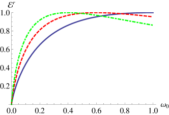
Figure 1: (color online) Left: Loop on the sphere of radius $\Omega$ in the parameter space which produces the desired logical operator with $\eta=\pi/2$. In the calculation of the integral (15) the loop begins in $(\theta_{m},0)$ (with $\theta_{m}$ near to the north pole), the evolution is along a meridian up to $(\theta_{M},0)$, then along a parallel up to $(\theta_{M},\phi_{M})$, along a meridian again up to $(\theta_{m},\phi_{M})$ and finally along a parallel back to $(\theta_{m},0)$. We recover the desired loop, that starts and ends at the north pole, in the limit $\theta_{m}\rightarrow 0$. The angle variables are supposed to depend linearly on time. Right: Entanglement as a function of $\omega_{0}$, for $\alpha=0$, with $\omega_{1}=0.4$ (dot-dashed), $0.6$ (dashed), $1$ (solid line).

Under the adiabatic condition $\Omega T\gg 1$, the adiabatic theorem guarantees that any superposition of the dark states at $t=0$ will end up in another superposition of dark states at $t=T$, and that this transformation is realized by the unitary holonomic operator DCZ

$$U_{0}(T)={\mathcal{T}}e^{-\int_{0}^{T}dt{A}(t)}\;,$$ (11)

obtained from (5) in the adiabatic limit ${\Omega}T\gg 1$; ${A}(t)$ in (11) is the connection operator with matrix elements

$$A_{ij}(t)=\langle D_{i}(t)|\frac{d}{dt}|D_{j}(t)\rangle\,,\quad{}i,j=1,2\,.$$ (12)

Equation (11) is the core of the holonomic approach to quantum computation: in view of (7), (8) and (11), the states $|0\rangle$ and $|1\rangle$ can be regarded as logical states spanning the two-dimensional logical space $\mathcal{L}_{A}\subset\mathcal{H}_{A}$ (the “A-qubit”) on which $U_{0}(T)$ acts as logical operator.

The main feature of the holonomic approach consists in the fact that $U_{0}(T)$ depends only on the area spanned by the curve (6). To see how this comes about, let us evaluate the RHS of (11): for the matrix (12) one finds

$$A(t)=\left(\begin{array}[]{cc}0&-\dot{\phi(t)}\cos\theta(t)\\ \dot{\phi(t)}\cos\theta(t)&0\end{array}\right)$$ (13)

whence,

$$U_{0}(T)=\left(\begin{array}[]{cc}\cos\eta&\sin\eta\\ -\sin\eta&\cos\eta\end{array}\right)\,,$$ (14)

where

$$\eta=\int_{0}^{T}dt\dot{\phi(t)}\cos\theta(t)$$ (15)

is the solid angle spanned on the sphere during the evolution. Therefore, if one wishes to construct, for example, a logical NOT operation, one has just to drive the external fields in such a way that the closed curve (6) spans a solid angle $\eta=\pi/2$. In fact, for this value of $\eta$ , the matrix (14) does what a NOT should do, namely, it exchanges the logical qubits $|0\rangle$ and $|1\rangle$ (modulo a sign).

In order to evaluate the integral (15), we proceed in the following way:

1. We choose a curve as in Fig. 1 consisting in a sequence of evolutions along meridians and parallels where $\theta_{M}$, $\phi_{M}$ are the maximal angles spanned during the evolution. Therefore, the solid angle spanned by the curve is $\eta=\phi_{M}(1-\cos\theta_{M})$.

2. Since the north pole of the sphere is a singular point of the parametrization (6), we choose a loop along meridians and parallels which starts (and ends) at the angles $(\theta_{m},0)$, (Fig. 1). The value of the integral for the loop starting and ending at the north pole, is recovered in the limit $\theta_{m}\rightarrow 0$ loopnote .

We shall now include the effect of parametric noise in the model. In view of the adiabatic evolution, it is reasonable to assume that the lasers are stable up to a relative error in the ratio between noise and signal. Thus the effect of an imprecise control of the driving fields is easily modeled by replacing the Rabi frequencies $\Omega_{i}(t)$ in (1) with $\widetilde{\Omega}_{i}(t)=\Omega_{i}(t)+\delta\Omega_{i}(t)$, where $\delta\Omega_{i}(t)$ are random fluctuations proportional to the intensities $\Omega_{i}(t)$ with $\delta\Omega_{i}(t)\ll\Omega_{i}(t)$. (From now on, for easiness of notation, we shall omit the explicit time dependence in the formulas and write, e.g., $\delta\Omega_{i}$ instead of $\delta\Omega_{i}(t)$.)

To compute the perturbed geometric operator $\widetilde{U}(T)$ by means of the perturbed connection $\widetilde{A}$, we pass from the Cartesian coordinates $\Omega_{i}+\delta\Omega_{i}$ to the spherical ones,

$$\widetilde{\Omega} = \Omega+\Delta\Omega\,,$$

$$\widetilde{\theta} = \theta+\Delta\theta\,,$$

$$\widetilde{\phi} = \phi+\Delta\phi\,.$$ (16)

From (6),

$$\widetilde{\Omega} = \sqrt{\sum_{i}(\Omega_{i}+\delta\Omega_{i})^{2}}\,,$$

$$\widetilde{\theta} = \arccos\left(\frac{\Omega_{a}+\delta\Omega_{a}}{\Omega+\delta\Omega}\right)\,,$$

$$\widetilde{\phi} = \arctan\left(\frac{\Omega_{0}+\delta\Omega_{0}}{\Omega_{1}+\delta\Omega_{1}}\right)\,.$$ (17)

By straightforward computation, one obtains the series expansion for $\Delta\Omega$, $\Delta\theta$ and $\Delta\phi$ in the small parameters $\delta\Omega_{i}\ll\Omega_{i}$

$$\Delta{\Omega} = \delta\Omega+\delta^{2}\Omega+O(\delta^{3})\,,$$

$$\Delta{\theta} = \delta\theta+\delta^{2}\theta+O(\delta^{3})\,,$$

$$\Delta{\phi} = \delta\phi+\delta^{2}\phi+O(\delta^{3})\;.$$ (18)

Here the “$\delta^{n}$”-terms collect terms of order $n$ in $\delta\Omega_{i}$, e.g.,

$$\delta\theta = \frac{\delta\Omega_{0}\Omega_{0}\Omega_{a}+\delta\Omega_{1}\Omega_{1}\Omega_{a}+\delta\Omega_{a}\left(\Omega_{a}^{2}-\Omega^{2}\right)}{\Omega^{2}\sqrt{\Omega_{0}^{2}+\Omega_{1}^{2}}}\,,$$

$$\delta\phi = \frac{\Omega_{0}\delta\Omega_{1}-\Omega_{1}\delta\Omega_{0}}{\Omega_{0}^{2}+\Omega_{1}^{2}}\,.$$ (19)

The perturbed solid angle is written as

$$\widetilde{\eta}=\eta+\delta\eta+\delta^{2}\eta+O(\delta^{3})\,,$$

with first order correction

$$\delta\eta=-\int_{0}^{T}dt(\dot{\phi}\delta\theta\sin\theta+\delta\dot{\phi}\cos\theta)\,.$$ (20)

The perturbed dark states $|\widetilde{D}_{i}\rangle$ are easily obtained from (4) by replacing $\Omega_{i}$ with $\widetilde{\Omega}_{i}$. Up to the second order in $\delta\Omega_{i}$ and at the final time $t=T$, one finds

$$|\widetilde{D}_{1}\rangle = \left(1-\frac{1}{2}\delta^{2}\theta-\frac{1}{2}\delta^{2}\phi\right)|D_{1}\rangle$$

$$+ (\delta\phi+\delta^{2}\phi)|D_{2}\rangle-\frac{\delta\theta+\delta^{2}\theta}{\sqrt{2}}\left(|B_{1}\rangle+|B_{2}\rangle\right)\,,$$

$$|\widetilde{D}_{2}\rangle = -(\delta\phi+\delta^{2}\phi)|D_{1}\rangle+(1-\frac{\delta^{2}\phi_{1}}{2})|D_{2}\rangle\,.$$ (21)

Note that $|\widetilde{D}_{1}\rangle$ is a superposition of both unperturbed dark and bright states thus leading to a population leakage from the unperturbed dark space to the unperturbed bright space.

The perturbed final operator $\widetilde{U}(T)$, written in the basis $\{|\widetilde{D}_{1}\rangle,|\widetilde{D}_{2}\rangle\}$, can be read directly from equation (14), by replacing $\eta$ with $\widetilde{\eta}=\eta+\delta\eta$. In particular, for $\eta=\pi/2$, up to second order,

$$\widetilde{U}(T)=\left(\begin{array}[]{ll}-\delta\eta-\delta^{2}\eta&\quad 1-\frac{(\delta\eta)^{2}}{2}\\ \\ -1+\frac{(\delta\eta)^{2}}{2}&\quad-\delta\eta-\delta^{2}\eta\end{array}\right)\,.$$ (22)

III Entanglement in multilevel systems

We shall now analyze a two-qubit system. We begin by specifying the model that we shall investigate:

1. We consider the composite system formed by two replicas of the system considered in the previous section—one will be called system A and the other system B. The Hilbert space of the composite is then $\mathcal{H}_{A}\otimes\mathcal{H}_{B}$, where $\mathcal{H}_{B}$, the Hilbert space of system B, is a replica of $\mathcal{H}_{A}$.

2. The logical space of the composite is $\mathcal{L}_{A}\otimes\mathcal{L}_{B}$, where, as before, $\mathcal{L}_{A}$ is the logical space of system A, spanned by the logical states $|0\rangle$ and $|1\rangle$, and $\mathcal{L}_{B}$ is the replica of $\mathcal{L}_{A}$ contained in $\mathcal{H}_{B}$. Following the standard terminology, we shall call $\mathcal{L}_{A}$ the A-qubit and $\mathcal{L}_{B}$ the B-qubit.

3. We shall assume that only the A-qubit undergoes information processing (for sake of concreteness, we shall assume that the A-qubit performs a logical NOT operation).

4. The initial state of the system is taken to be the maximally entangled state

   $$\Psi=\frac{1}{\sqrt{2}}(|00\rangle+|11\rangle)\,.$$ (23)

We note that the relevant simplifying assumption is 3, while 4 is rather standard for the kind of problem we wish to address here (see below). Note that assumption 3 allows two possibilities for representing the time evolution of the two-qubit system:

• a unitary transformation of the form $U\otimes I$, where $U$ governs the dynamics of the system A (e.g., as given by (22)), and $I$ is the identity in $\mathcal{H}_{B}$;

• a unitary transformation which accounts for the interaction between the two qubits.

Case a) will be addressed in this section and case b) in Sect. V.

Our aim is to study how the entanglement of the two qubits is preserved by the dynamics and to do this we need a quantitative estimate of the entanglement.

When a system is composed by two sub-systems A and B, the entanglement of the composite system, in the case of pure states, can be estimated in terms of the von Neumann entropy

$$\mathcal{E}=-\mbox{Tr}(\rho_{A}\log_{2}\rho_{A})=-\mbox{Tr}(\rho_{B}\log_{2}\rho_{B})\,.$$ (24)

where $\rho_{A}$ and $\rho_{B}$ are the reduced density matrices of the sub-systems wootters . However, since in our model the qubits are embedded in a larger space, formula (24) cannot be directly applied.

To arrive at a suitable estimator of entanglement, we proceed as follows: Let $P$ denote the projector on the logical subspace $\mathcal{L}_{A}$ of $\mathcal{H}_{A}$ and let $P\otimes P$ be the projector onto $\mathcal{L}_{A}\otimes\mathcal{L}_{B}$. Consider

$$\rho^{r}=P\otimes P\rho P\otimes P$$ (25)

and

$$\rho_{A}^{r}=\mbox{Tr}_{B}\rho^{r}\,.$$ (26)

Then the quantity

$$\mathcal{E}^{r}=-\mbox{Tr}(\rho_{A}^{r}\log_{2}\rho_{A}^{r})\,,$$ (27)

is analogous to (24), and can be regarded as an estimator of the fraction of entanglement in the logical subspace (see also nihira-stroud ). Hereafter we shall refer to to $\mathcal{E}^{r}$ as the reduced logical entanglement or, when no ambiguity will arise, simply as the entanglement.

We wish now to obtain a convenient formula for $\mathcal{E}^{r}$ (under the assumption a) specified above). Firstly, we evaluate

$$\rho_{A}^{r}=\mbox{Tr}_{B}\left(P\otimes PU\otimes I|\Psi\rangle\langle\Psi|U^{*}\otimes IP\otimes P\right)$$ (28)

without relying on any specific form of the unitary $U$. To this end we note that a generic transformation $U$ of the logical qubit basis can be written as

$$U|0\rangle = PU|0\rangle+P^{\perp}U|0\rangle$$

$$U|1\rangle = PU|1\rangle+P^{\perp}U|1\rangle\;.$$ (29)

Let

$$\sqrt{\omega_{0}}=\left\|PU|0\rangle\right\|\;,\;\;\sqrt{\omega_{1}}=\left\|PU|1\rangle\right\|$$ (30)

and denote by $|\psi_{0}\rangle$, $|\psi_{1}\rangle$, $|\psi_{0}^{\bot}\rangle$, and $|\psi_{1}^{\bot}\rangle$ the vectors obtained by normalization from $PU|0\rangle$, $PU|1\rangle$, $P^{\bot}U|0\rangle$, and $P^{\perp}U|1\rangle$ respectively. Then

$$U|0\rangle = \sqrt{\omega_{0}}|\psi_{0}\rangle+\sqrt{1-\omega_{0}}|\psi_{0}^{\bot}\rangle$$

$$U|1\rangle = \sqrt{\omega_{1}}|\psi_{1}\rangle+\sqrt{1-\omega_{1}}|\psi_{1}^{\bot}\rangle\,.$$ (31)

It is useful to introduce the scalar product

$$\alpha=\langle\psi_{0}|\psi_{1}\rangle\,.$$ (32)

Note that the coefficients $\sqrt{1-\omega_{i}}$ represent the leakage of the populations and that in general $\alpha$ is different from zero. Therefore

$$U\otimes I|\Psi\rangle = \frac{1}{\sqrt{2}}\left[\sqrt{\omega_{0}}|\psi_{0}0\rangle+\sqrt{1-\omega_{0}}|\psi_{0}^{\bot}0\rangle\right.$$ (33)

$$\left.+\sqrt{\omega_{1}}|\psi_{1}1\rangle+\sqrt{1-\omega_{1}}|\psi_{1}^{\bot}1\rangle\right]\,,$$

and

$$PU\otimes I|\Psi\rangle=\frac{1}{\sqrt{\omega_{0}+\omega_{1}}}[\sqrt{\omega_{0}}|\psi_{0}0\rangle+\sqrt{\omega_{1}}|\psi_{1}1\rangle]\,.$$ (34)

Noting that $|\psi_{1}\rangle$ can be decomposed into its components along and orthogonal to $|\psi_{0}\rangle$: $|\psi_{1}\rangle=\alpha|\psi_{0}\rangle+\beta|\widetilde{\psi}_{0}\rangle$ with $\langle\psi_{0}|\widetilde{\psi}_{0}\rangle=0$, $\alpha$ given in (32), and $\beta=\sqrt{1-\alpha^{2}}$, we find

$$PU\otimes I|\Psi\rangle=\frac{\sqrt{\omega_{0}}|\psi_{0}0\rangle+\alpha\sqrt{\omega_{1}}|\psi_{0}1\rangle+\beta\sqrt{\omega_{1}}|\widetilde{\psi}_{0}1\rangle}{\sqrt{\omega_{0}+\omega_{1}}}\,.$$ (35)

Thus, we may evaluate (28) in the $\{|\psi_{0}\rangle\,,|\widetilde{\psi}_{0}\rangle\}$ basis,

$$\rho_{A}^{r}=\frac{1}{\omega_{0}+\omega_{1}}\left(\begin{array}[]{ll}\omega_{1}\alpha^{2}+\omega_{0}&\quad\alpha\sqrt{1-\alpha^{2}}\omega_{1}\\ \\ \alpha\sqrt{1-\alpha^{2}}\omega_{1}&\quad-\left(\alpha^{2}-1\right)\omega_{1}\end{array}\right)\,,$$ (36)

whence

$$\mathcal{E}^{r}=-(\lambda_{-}\log_{2}\lambda_{-}+\lambda_{+}\log_{2}\lambda_{+})\,,$$ (37)

where

$$\lambda_{\pm}=\frac{\omega_{0}+\omega_{1}\pm\sqrt{\omega_{0}^{2}+2\left(2\alpha^{2}-1\right)\omega_{1}\omega_{0}+\omega_{1}^{2}}}{2\left(\omega_{0}+\omega_{1}\right)}$$ (38)

are the eigenvalues of $\rho_{A}^{r}$.

In Fig. 1 (right), $\mathcal{E}^{r}$ is plotted as a function of $\omega_{0}$ for $\alpha=0$ and different values of $\omega_{1}$. It follows immediately from (37) and (38) that $\mathcal{E}^{r}=1$ for $\alpha=0$ and $\omega_{0}=\omega_{1}$ (this includes the trivial case of no leakage for which $\omega_{0}=\omega_{1}=1$, as well as non-trivial cases of population leakage with $\omega_{0}=\omega_{1}<1$). For $\alpha\neq 0$, it is always $\mathcal{E}^{r}<1$.

We now specialize to the case $U=\widetilde{U}(T)$, with $\widetilde{U}(T)$ given by (22). Keeping the contributions up to the second order in the perturbations $\delta\Omega_{i}$, we obtain

$$P\widetilde{U}(T)|0\rangle = \sqrt{\omega_{0}}|\psi_{0}\rangle=\left(\delta\phi+\delta^{2}\phi-\delta\eta-\delta^{2}\eta\right)|0\rangle$$

$$+\left(\frac{\delta\phi^{2}}{2}-\delta\eta\delta\phi+\frac{(\delta\eta)^{2}}{2}-1\right)|1\rangle$$

$$P^{\perp}\widetilde{U}(T)|0\rangle = \sqrt{1-\omega_{0}}|\psi_{0}^{\bot}\rangle=\frac{\delta\theta\delta\eta}{\sqrt{2}}\left(|a\rangle+|G\rangle\right)$$

$$P\widetilde{U}(T)|1\rangle = \sqrt{\omega_{1}}|\psi_{1}\rangle$$

$$= \Big{(}1-\frac{\delta\theta^{2}}{2}-\frac{\delta\phi^{2}}{2}-\frac{(\delta\eta)^{2}}{2}+\delta\phi\delta\eta\Big{)}|0\rangle$$

$$+ \Big{(}\delta\phi+\delta^{2}\phi-\delta\eta-\delta^{2}\eta\Big{)}|1\rangle$$

$$P^{\perp}\widetilde{U}(T)|1\rangle = \sqrt{1-\omega_{1}}|\psi_{1}^{\bot}\rangle$$ (39)

$$= -\frac{\delta\theta+\delta^{2}\theta}{\sqrt{2}}\left(|a\rangle+|G\rangle\right)$$

and

$$\alpha = O(\delta^{3})$$

$$\omega_{0} = 1+O(\delta^{4})$$

$$\omega_{1} = 1-\frac{(\delta\theta)^{2}}{8}+O(\delta^{3})\,.$$ (40)

In the above equations $\delta\theta$ and $\delta\phi$ are evaluated at $t=T$. From (6) and (19) it follows that $\delta\theta=0$ and that one can set $\delta\phi=0$. Thus $\alpha=0$ and $\omega_{0}=\omega_{1}=1$, whence, as above, $\mathcal{E}^{r}=1$.

IV Fidelity

If the system is subject to noise sources, the fidelity $\mathcal{F}$ is used to quantify the “distance” between the perturbed final state $\mathcal{U}(T)\Psi$, due to a perturbed evolution $\mathcal{U}$, and the final unperturbed state $U_{0}(T)\otimes I\Psi$, with $U_{0}(T)$ given by (14). For composite systems, $\mathcal{F}$ provides an estimation of the performance of logical operators that supplement the information already provided by $\mathcal{E}^{r}$. The explicit formula for the fidelity is

$$\mathcal{F}=\left|\langle\mathcal{U}(T)\Psi|U_{0}(T)\otimes I\Psi\rangle\right|\,.$$ (41)

For the case we wish to consider first, $\mathcal{U}(T)=\widetilde{U}(T)\otimes I$, with $\widetilde{U}(T)$ given by (22). From (39), by a straightforward computation, one obtains

$$\mathcal{F}=1-\frac{(\delta\theta)^{2}}{4}-\frac{(\delta\phi)^{2}}{2}-\frac{(\delta\eta)^{2}}{2}+\delta\phi\delta\eta+O(\delta^{3})\,.$$ (42)

Since, the terms $\delta\theta$ and $\delta\phi$ are evaluated at time $T$, their contribution is zero and thus

$$\mathcal{F}\approx 1-\frac{(\delta\eta)^{2}}{2}\,.$$ (43)

The fidelity depends on the error $\delta\eta$ relative to the area spanned during the perturbed evolution, it then appears to be less robust than entanglement.

We shall now estimate $\delta\eta$ for a simple model of noise. We first integrate by parts the second term in Eq. (20) neglecting the contribution at the endpoints

$$\delta\eta=-\int dt(\dot{\phi}\delta\theta+\dot{\theta}\delta\phi)\sin\theta\,.$$ (44)

We consider the loop in Fig. 1 passing near the north pole and then take the limit for $\theta_{m}\rightarrow 0$, in the notation of the figure caption. We separate the contribution of four different parts depending on the evolution along meridians and parallels (cf. Fig. 1) and denote by $\int_{i}f(t)dt$ the contribution along the $i$th path. We have

$$\delta\eta = -\int_{1,3}dt\dot{\theta}\delta\phi\sin\theta-\sin\theta_{M}\int_{2}dt\dot{\phi}\delta\theta$$ (45)

$$-\sin\theta_{m}\int_{4}dt\dot{\phi}\delta\theta\,.$$

Note that in the limit of $\theta_{m}\rightarrow 0$ the fourth integral gives no contribution. We now suppose that the perturbations $\delta\Omega_{i}$ fluctuate randomly over a time scale $\tau\ll T$ and go off whenever the driving fields are turned off, i.e. that they are of the form

$$\delta\Omega_{i}(t) = \Omega_{i}(t)Z_{i}(t)=$$ (46)

$$= \Omega_{i}(t)\sum_{k=0}^{n-1}h\left(\frac{t-k\tau}{\tau}\right)Z^{i}_{k}\,,$$

where $h(x)$ is the “box” function, which is equal to $1$ in the interval $0\leq x<1$ and zero elsewhere, $n=T/\tau$, and $Z^{i}_{k}$ are independent Gaussian random variables, with zero average and variance $\sigma^{2}$.

Using (6) and (19) we can explicitly write the contributions for the separate evolutions. Along the first meridian we have no contribution since $\phi=0$. The only non-zero contributions are along the second and third paths; we suppose that $\theta$ and $\phi$ depend linearly on time (see also loopnote ) and write $\dot{\theta}=v_{\theta}$ and $\dot{\phi}=-v_{\phi}$. We thus obtain

$$\delta\eta =v_{\phi}\cos\theta_{M}\sin^{2}\theta_{M}\int_{2}dt\left(Z_{0}\cos^{2}\phi+Z_{1}\sin^{2}\phi-Z_{a}\right)+$$

$$-\frac{v_{\theta}}{2}\sin 2\phi_{M}\int_{3}dt\left(Z_{0}-Z_{1}\right)\sin\theta\,.$$ (47)

Inserting (46) in (47) one can perform the integration and the expansion at first order in $\tau/T=1/n\ll 1$

$$\delta\eta =4\phi_{M}\cos\theta_{M}\sin^{2}\theta_{M}\times$$

$$\times\sum_{k=0}^{n-1}\Big{[}\frac{Z^{0}_{k}\cos^{2}(k\tau v_{\phi})}{n}-\frac{Z^{1}_{k}\sin^{2}(k\tau v_{\phi})}{n}-\frac{Z^{a}_{k}}{n}\Big{]}+$$

$$-2\left(\theta_{M}-\theta_{m}\right)\sin\left(2\phi_{M}\right)\sum_{k=0}^{n-1}\frac{\sin\left(k\tau v_{\theta}\right)\left(Z_{k}^{0}-Z_{k}^{1}\right)}{n}\,.$$ (48)

Using the independence of the random variables $Z_{k}^{i}$, from the central limit theorem it follows that for $n\gg 1$

$$(\delta\eta)^{2}\approx\frac{\sigma^{2}}{n}=\frac{\sigma^{2}\tau}{T}\,,$$ (49)

which expresses the cancellation effect already discussed in robustness_solinas for large $n$. Thus the fidelity (43) becomes

$$\mathcal{F}\approx 1-\frac{\sigma^{2}}{2}\frac{\tau}{T}\,.$$ (50)

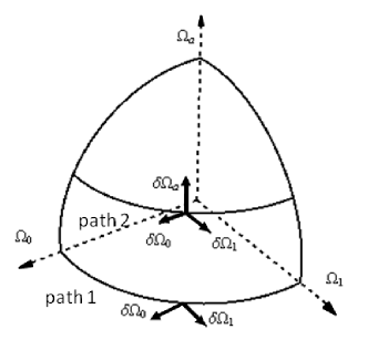
Figure 2: Evolution along the equator (path $1$ with $\theta_{M}=\pi/2$) and along a generic parallel (path $2$). In the first case, only the perturbation $\delta\Omega_{0}$ and $\delta\Omega_{1}$ for the laser turned on are present.

The above calculation is valid for any loop in the parameter space which moves along a parallel and meridian and spans a $\pi/2$ solid angle. Among these loops, there is one which is particularly interesting. If $\theta_{M}=\pi/2$ and $\phi_{M}=\pi/2$, we are moving on the $\Omega_{a}-\Omega_{0}$ plane, along the equator and on the $\Omega_{a}-\Omega_{1}$ plane. As can be seen from (47), with this loop the contributions along the second and third paths are zero and $\delta\eta=0$ independently of the characteristics of the noise (variance and correlation time). In other words, this loop makes the system completely robust against this particular perturbation. This fact has a simple geometrical and physical interpretation. We recall that the loop describes the way we turn on and off the lasers. The above loop is the one in which we have always one laser completely turned off while modulating the intensities of the other two; for example, in Fig. 2 is shown the evolution along the equator (path $1$) when $\Omega_{a}$ laser turned off and we are modulating the $\Omega_{0}$ and $\Omega_{1}$ intensities. Along this path, $\delta\Omega_{a}=0$ while we have perturbation of the other two lasers. However, the perturbations $\delta\Omega_{0}$ and $\delta\Omega_{1}$ produce only radial and $\delta\theta$ perturbation which do not affect the solid angle along this path. In other words, choosing this particular loop, along the single paths, we eliminate the part of perturbation which can modify the solid angle spanned and as result the angle is spanned without error.

V Coupled Qubits

In a more realistic situation, the two qubits can also interact. This interaction allows to manipulate the two systems as a whole and it is the basis for constructing two qubit gates. Ideally, one can control the coupling strength and turn it on and off depending on the logical gate. However, if the interaction cannot be perfectly turned off, its presence results in a new source of noise. Here, we choose to describe it with a simple model with

$$H_{I}=\chi|11\rangle\langle 11|\,.$$ (51)

As before, only the A qubit undergoes an information process. Due to the specific form of the coupling (51) only the state $|1\rangle$ of qubit B will feel the additional interaction. It is then convenient to analyze the evolution in the dark-bright basis for the qubit A and in the state $|1\rangle$ for the quit B: $\{|D_{1}1\rangle,|D_{2}1\rangle,|B_{1}1\rangle,|B_{2}1\rangle\}$ (neglecting, for the moment, additional errors induced by the imprecise control). If $\Omega\gg\chi$, and the system starts in a superposition of dark states, the transition to the bright states are negligible and the evolution stay in the dark space $\{|D_{1}1\rangle,|D_{2}1\rangle\}$. The Hamiltonian $H_{I}$ in this basis is

$$H_{I}=\chi\left(\begin{array}[]{ll}\cos^{2}\theta\sin^{2}\phi&\quad\cos\theta\cos\phi\sin\phi\\ \\ \cos\theta\cos\phi\sin\phi&\quad\cos^{2}\phi\end{array}\right).$$ (52)

Thus, one sees that $H_{I}$ breaks the energy degeneracy $E_{1}=E_{2}=0$ of the two dark states $|D_{1}\rangle$ and $|D_{2}\rangle$, relative to the unperturbed Hamiltonian (1). The new eigenvalues are easily evaluated by diagonalization in the presence of $H_{I}$,

$$\bar{E}_{1}=0\,,\quad\bar{E}_{2}=\chi(\cos^{2}\phi+\cos^{2}\theta\sin^{2}\phi)\,.$$ (53)

The corresponding eigenvectors can be written as a superposition of the unperturbed dark states

$$|{\bar{D}}_{1}(t)\rangle = \alpha(t)|D_{1}(t)\rangle-\beta(t)|D_{2}(t)\rangle$$

$$|{\bar{D}}_{2}(t)\rangle = \beta(t)|D_{1}(t)\rangle+\alpha(t)|D_{2}(t)\rangle\,,$$ (54)

with

$$\alpha(t) = \frac{\displaystyle{\cos\phi(t)}}{\displaystyle{\sqrt{\cos^{2}\phi(t)+\cos^{2}\theta(t)\sin^{2}\phi(t)}}}$$

$$\beta(t) = \frac{\displaystyle{\cos\theta(t)\sin\phi(t)}}{\displaystyle{\sqrt{\cos^{2}\phi(t)+\cos^{2}\theta(t)\sin^{2}\phi(t)}}}\,.$$ (55)

These coefficients satisfy boundaries conditions, related to the closed loop in Fig. (1) with $\theta(0)=\theta(T)=\phi(0)=\phi(T)=0$

$$\alpha(0)=\alpha(T)=1\,,\quad\beta(0)=\beta(T)=0\,,$$ (56)

and normalization

$$\alpha^{2}(t)+\beta^{2}(t)=1.$$ (57)

Note that the energy shift (53), induced by the perturbation, may produce important modifications during the time evolution since non-Abelian effects are based on the assumption of degeneracy. If $\chi T\gg 1$ the perturbed dark states are separated during the evolution and no holonomic operator (11) can be produced. For this reason we shall focus, in the following, on the more relevant case $\chi T\leq 1$, which preserve the logical space.

The evolution operator is now

$$U_{\chi}(T)=\mathcal{T}e^{-i\int_{0}^{T}\left[H_{I}(t)-i\bar{A}(t)\right]dt}\,.$$ (58)

(Note that the first term in the exponential, which represents the dynamic contribution of the perturbed dark states, is absent in (11) since there the dark states are degenerate). Using the new basis $\{|{\bar{D}(t)}_{1}1\rangle,|{\bar{D}(t)}_{2}1\rangle\}$,

$$\bar{A}_{ij}(t)=\langle{\bar{D}}_{i}(t)1|\frac{d}{dt}|{\bar{D}}_{j}(t)1\rangle\quad i,j=1,2\,,$$

and thus

$$\bar{A(t)}=\left(\begin{array}[]{ll}\alpha\dot{\alpha}+\beta\dot{\beta}&\quad\beta\dot{\alpha}-\alpha\dot{\beta}-\cos\theta\dot{\phi}\\ \alpha\dot{\beta}-\beta\dot{\alpha}+\cos\theta\dot{\phi}&\quad\alpha\dot{\alpha}+\beta\dot{\beta}\end{array}\right)\,.$$ (59)

The integral $\int_{0}^{T}\bar{A}(t)dt$ in (58) can be evaluated using (55), (56) and (57). The integrals of the diagonal terms in (59) are always zero because they represent the derivative of the norm of the dark states, which is time independent. For the off-diagonal part, it can be easily shown that $\alpha\dot{\beta}-\beta\dot{\alpha}=\dot{\alpha}/(1-\alpha^{2})^{1/2}$ gives no contribution once it is integrated along the closed loop. Thus

$$\int_{0}^{T}\bar{A}(t)dt=\left(\begin{array}[]{ll}0&\quad-\eta\\ \eta&\quad\;0\end{array}\right)\,.$$ (60)

The integral $\int_{0}^{T}H_{I}(t)dt$ in (58) can be evaluated by performing the integration along the loop shown in Fig. 1 with constant velocities. One obtains

$$\int_{0}^{T}H_{I}(t)dt=\int_{0}^{T}\bar{E}_{2}dt=\chi T\gamma(\theta_{M},\phi_{M})$$ (61)

with

$$\gamma(\theta_{M},\phi_{M}) = \frac{1}{3}+\frac{\sin 2\theta_{M}\sin^{2}\phi_{M}+\left(3+\cos 2\phi_{M}\right)\theta_{M}}{12\theta_{M}}$$ (62)

$$+ \frac{\sin 2\phi_{M}\sin^{2}\theta_{M}+\left(3+\cos 2\theta_{M}\right)\phi_{M}}{12\phi_{M}}\,.$$

Here, $\theta_{M}$ and $\phi_{M}$ satisfy $\phi_{M}(1-\cos\theta_{M})=\eta$, with $\eta$ the solid angle spanned on the sphere during the evolution given in (15).

From (60) and (61), one may evaluate the RHS of (58) and obtain, in the logical basis $\{|0\rangle,|1\rangle\}$, the matrix

$$U_{\chi}(T)=\frac{1}{\mu}\left(\begin{array}[]{ll}e^{i\frac{\chi T\gamma}{2}}K_{-}&\quad 2e^{i\frac{\chi T\gamma}{2}}\eta\sin\frac{\mu}{2}\\ \\ -2e^{i\frac{\chi T\gamma}{2}}\eta\sin\frac{\mu}{2}&\quad e^{i\frac{\chi T\gamma}{2}}K_{+}\end{array}\right),$$ (63)

where

$$K_{\pm}=\left(\mu\cos\frac{\mu}{2}\pm i\chi T\gamma\sin\frac{\mu}{2}\right),\quad\mu=\sqrt{4\eta^{2}+(\chi T\gamma)^{2}}\,.$$ (64)

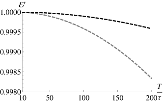
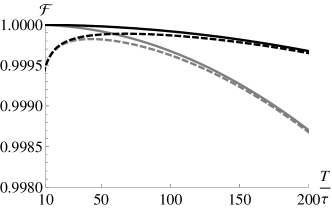
Figure 3: Left: Entanglement as a function of $T/\tau$ for $\sigma=0.1$ and $\chi\tau=10^{-3}$ (grey dashed line); $\chi\tau=5~{}10^{-4}$ (black dashed line). Right: Fidelity as a function of $T/\tau$ for $\sigma=0$ and $\chi\tau=10^{-3}$ (grey solid line), $\sigma=0$ and $\chi\tau=5~{}10^{-4}$ (black solid line), $\sigma=0.1$ and $\chi\tau=10^{-3}$ (grey dashed line), $\sigma=0.1$ and $\chi\tau=5~{}10^{-4}$ (black dashed line). In all the plots the loop is as in Fig. 1 and with the choosen $\theta_{M}$ and $\phi_{M}$ we have $\gamma=0.75$.

We shall consider as initial state the maximally entangled state (23). From (7), (8), (23) and (54) it follows that

$$|\Psi\rangle=\frac{1}{\sqrt{2}}(|{\bar{D}}_{1}(0)0\rangle+|{\bar{D}}_{2}(0)1\rangle)\,.$$ (65)

Note that the time evolution of $|{\bar{D}}_{1}(0)0\rangle$ is driven by the unitary operator $U_{0}(T)$ in (14), since the interaction does not affect the state $|0\rangle$ of qubit B. On the other hand, $|{\bar{D}}_{2}(0)1\rangle$ evolves with the perturbed unitary operator $U_{\chi}(T)$ in (63). Thus, to study the evolution of $\Psi$ it is useful to introduce the operator

$$\mathcal{U}(T)=U_{0}(T)\otimes\left(\begin{array}[]{ll}1&0\\ 0&0\end{array}\right)+U_{\chi}(T)\otimes\left(\begin{array}[]{ll}0&0\\ 0&1\end{array}\right)\,.$$ (66)

Here, as usual, $U_{0}(T)$ and $U_{\chi}(T)$ act on the qubit A, while the other two matrices act on the qubit B and are expressed in the $|0\rangle,|1\rangle$ basis for B. Then

$$\mathcal{U}(T)|{\bar{D}}_{1}(0)0\rangle\!\! = \!\!\cos\eta|00\rangle-\sin\eta|10\rangle$$

$$\mathcal{U}(T)|{\bar{D}}_{2}(0)1\rangle\!\! = \!\frac{e^{i\frac{\chi T\gamma}{2}}}{\mu}\!\!\left(2\eta\sin\frac{\mu}{2}|01\rangle+K_{+}\!|11\rangle\right)$$ (67)

Let us now evaluate (26) at $t=T$,

$$\rho_{A}^{r}=\mbox{Tr}_{B}\left(P\otimes P\mathcal{U}(T)|\Psi\rangle\langle\Psi|\mathcal{U}^{*}(T)P\otimes P\right)\,,$$ (68)

and thus, from (66),

$$\rho_{A}^{r}=\frac{1}{2\mu}\left(\begin{array}[]{ll}\qquad\mu&\quad e^{-\frac{i\chi T\gamma}{2}}\left(2\eta\cos\eta\sin\frac{\mu}{2}-K_{-}\sin\eta\right)\\ \\ e^{\frac{i\chi T\gamma}{2}}\left(2\eta\cos\eta\sin\frac{\mu}{2}-K_{+}\sin\eta\right)&\quad\qquad\mu\end{array}\right).$$ (69)

The calculation of $\mathcal{E}^{r}$ is now straightforward by using (37) and (69). Here, we quote the lowest order expansions in the coupling $\chi$

$$\mathcal{E}^{r}=1-\frac{(\gamma\chi T)^{2}\sin^{4}(\eta)}{8\eta^{2}}+O((\chi T)^{3}))\,.$$ (70)

Note that the presence of the qubits coupling affects the entanglement inducing a quadratically decreasing behavior in $\chi$. Only in the limit $\eta\to 0$ (no holonomic transformation) the entanglement is still preserved, $\mathcal{E}^{r}=1$, irrespectively on the coupling. Indeed, in this case the time evolved state, starting from a maximally entangled state (65) differs from the initial state by a phase factor $|\Psi(T)\rangle=(|00\rangle+\exp(-i\chi T)|11\rangle)/\sqrt{2}$, which does not affect the entanglement.

The fidelity (41) can now be evaluated for $\mathcal{U}(T)$ given by (66) (see also (67)). One finds

$$\mathcal{F} = 1-\left(7+8\eta^{2}+8\eta\sin(2\eta)-8\cos(2\eta)+\cos(4\eta)\right)\times$$ (71)

$$\times\frac{(\gamma\chi T)^{2}}{256\eta^{2}}+O((\chi T)^{3}))\,.$$

Note that, differently from the entanglement, even in the absence of holonomic transformation ($\eta=0$) the fidelity is affected by the coupling, i.e.,

$$\mathcal{F}|_{\eta=0}=1-\frac{(\gamma\chi T)^{2}}{8}+O((\chi T)^{3}))\,.$$

We shall now take into account the effect of the parametric noise and consider the case of a perturbation to the logical NOT operation with $\eta=\pi/2$. The perturbed unitary operator $\widetilde{U}_{\chi}$ is obtained from (63) by means of the substitutions

$$\eta \rightarrow \widetilde{\eta}=\frac{\pi}{2}+\delta\eta$$

$$\mu \rightarrow \widetilde{\mu}=\sqrt{(\pi+2\delta\eta)^{2}+(\chi T\gamma)^{2}}$$

$$K_{\pm} \rightarrow \widetilde{K}_{\pm}=\left(\tilde{\mu}\cos\frac{\tilde{\mu}}{2}\pm i\chi T\gamma\sin\frac{\widetilde{\mu}}{2}\right)$$

and the evolution operator which extends (66) is

$$\widetilde{\mathcal{U}}(T)=\widetilde{U}(T)\otimes\left(\begin{array}[]{ll}1&0\\ 0&0\end{array}\right)+\widetilde{U}_{\chi}(T)\otimes\left(\begin{array}[]{ll}0&0\\ 0&1\end{array}\right)$$ (72)

with $\widetilde{U}(T)$ given in Eq. (22), whence

$$\rho_{A}^{r}=\frac{1}{2\widetilde{\mu}}\left(\begin{array}[]{ll}\qquad\qquad\tilde{\mu}&-e^{-\frac{i\chi T\gamma}{2}}\left[\widetilde{K}_{-}\cos\delta\eta+2\tilde{\eta}\sin\delta\eta\sin\frac{\tilde{\mu}}{2}\right]\\ -e^{\frac{i\chi T\gamma}{2}}\left[\widetilde{K}_{+}\cos\delta\eta+2\tilde{\eta}\sin\delta\eta\sin\frac{\tilde{\mu}}{2}\right]\qquad\qquad\tilde{\mu}\end{array}\right).$$ (73)

Thus, from (37), (41), and (73), we finally obtain (at the lowest orders in the errors)

$$\mathcal{E}^{r} \approx 1-\frac{\left(\pi-4\delta\eta\right)(\gamma\chi T)^{2}}{2\pi^{3}}$$ (74)

$$\mathcal{F} \approx 1-\frac{(\delta\eta)^{2}}{2}-\frac{\left(8+\pi^{2}\right)(\gamma\chi T)^{2}}{32\pi^{2}}\,.$$ (75)

It should be observed that $\mathcal{E}^{r}$ is jointly reduced by coupling $\chi$ and parametric noise $\delta\eta$ (yet $\mathcal{E}^{r}=1$ for $\chi=0$ and $\delta\eta\neq 0$, in agreement with the results of Sec. III), and that the parametric noise may increase the entanglement with respect to the bare case with $\eta=\pi/2$ (in accordance with the behavior discussed in Eq. (70), where $\mathcal{E}^{r}\to 1$ for $\eta\to 0$). Moreover, note that the fidelity $\mathcal{F}$ is influenced independently by the two sources of noise. Indeed, in addition to the decrease induced by the coupling, already accounted by (71), the fidelity is also depressed by the geometric perturbation $\delta\eta$ in agreement with the results in Sec. III.

The model of parametric noise introduced in Sec. IV allows for a more quantitative analysis of (74) and (75). According to this model, $\delta\eta=\sigma\sqrt{\tau/T}$ (cf. Eq (49)), with $\sigma^{2}$ the variance and $\tau$ the time scale of the noise fluctuations; the condition of small perturbations, $\delta\eta\ll\pi/2$, implies $\sigma\sqrt{\tau/T}\ll\pi/2$. The behaviors of entanglement and fidelity are represented in Fig. 3; more precisely:

• Fig. 3 (left) shows the entanglement (74) as a function of the final time $T$ for fixed $\sigma$ and different values of $\chi\tau$. The value of $\gamma$, defined in (62), depends on the loop chosen with $0.66\leq\gamma\leq 1$. Here, $\gamma=0.75$. The behavior suggests a way to preserve entanglement: choosing not too long evolution times the dominant source of error can be minimized. In particular an evolution with $T<200\tau$ causes an error on the entanglement smaller than $1.5~{}10^{-3}$.

• Fig. 3 (right) shows the fidelity. When $\sigma=0$, i.e. no parametric error, the fidelity shows a quadratically decreasing behavior as a function of $T/\tau$ depending on the values of $\chi\tau$ (solid lines). The presence of a parametric noise changes qualitatively the behavior for small $T/\tau$. In fact, in this region independently of the $\chi$ coupling, the fidelity drops because the geometric error dominates. By increasing $T/\tau$ there is an intermediate region where the fidelity increases before fast decreasing, when the $\chi$ error prevails. Intermediate times evolution are then the more efficient to preserve the fidelity. A good choice is $50\tau<T<100\tau$. In this range of adiabatic times, both entanglement and fidelity have errors of order $5~{}10^{-4}$.

To conclude, the constraints on the time scales of our model that allow to construct holonomic gates which preserve both entanglement and fidelity and are consistent with the adiabatic approximation are:

$$\Omega^{-1}<50\tau<T<100\tau<\chi^{-1}$$ (76)

with the additional request that $\sigma\ll\sqrt{50}\pi/2$.

VI Conclusions

In the present paper we studied a noisy two-qubit system in order to understand if and how the holonomic operators preserve the entanglement. We considered a model in which only one of the two qubits undergoes a holonomic transformation. Being the two dimensional logical space embedded in an extended four dimensional Hilbert space we introduced, as possible estimator, the reduced logical entanglement which correponds to the fraction of entanglement in the logical subspace. We also calculated the fidelity and compared it with the reduced logical entanglement.

We considered two types of noise: a parametric noise that goes off whenever the driving fields are turned off, and a coupling noise due to undesired interactions between the two qubits. We have shown that the holonomic operators are robust under parametric error. In particular, the entanglement is preserved under an holonomic transformations while the fidelity is affected by such a noise but, due to geometric cancellation effects, it can reach good values for long times. In the presence also of a coupling error, we showed that the entanglement is mainly influenced by this noise and weakly by the geometric perturbation. Instead, the fidelity shows a different dependence on the adiabatic time: it is dominated by the parametric noise for not too large times and depends on the coupling error at larger times. We demonstrated that the intermediate time evolutions are the best choice. Within a realistic range of physical parameters, we found that for both entanglement and fidelity the error can be strongly reduced.

Acknowledgments

We thank E. De Vito and A. Toigo for many fruitful discussions. N. Zanghì was supported in part by INFN.

References

(1) L. Amico, R. Fazio, A. Osterloh, and V. Vedral,
Rev. Mod. Phys. 80, 517 (2008).
(2)
L.-M. Duan and G.-C. Guo, Phys. Rev. A 57, 737 (1998).
(3)
A. R. Carvalho, F. Mintert, and A. Buchleitner, Phys. Rev. Lett. 93, 230501 (2004).
(4) J.-M. Cai, Z.-W. Zhou, and G.-C. Guo, Phys. Rev. A 72, 022312 (2005).
(5)
J. A. Jones, V. Vedral, A. Ekert, and G. Castagnoli, Nature (London) 403, 869 (2000).
(6)
G. Falci, R. Fazio, G. M. Palma, J. Siewert, and V. Vedral, Nature (London) 407, 355 (2000).
(7) D. Leibfried et al., Nature 422, 412 (2003).
(8)R. G. Unanyan, B.W. Shore, and K. Bergmann, Phys. Rev. A 59, 2910 (1999).
(9) L.-M. Duan, J.I. Cirac, and P. Zoller, Science 292, 1695 (2001).
(10) L. Faoro, J. Siewert, and R. Fazio, Phys. Rev. Lett. 90, 028301 (2003).
(11) I. Fuentes-Guridi, J. Pachos, S. Bose, V. Vedral, and S. Choi,
Phys. Rev. A 66, 022102 (2002).
(12) A. Recati, T. Calarco, P. Zanardi, J. I. Cirac, and P. Zoller,
Phys. Rev. A 66, 032309 (2002).
(13) P. Solinas, P. Zanardi, N. Zanghì, and
F. Rossi, Phys. Rev. B 67, 121307(R) (2003).
(14) A. Carollo, I. Fuentes-Guridi, M. F. Santos, and
V. Vedral, Phys. Rev. Lett. 90, 160402 (2003).
(15) G. De Chiara and G. M. Palma, Phys. Rev. Lett. 91, 090404 (2003).
(16) A. Carollo, I. Fuentes-Guridi, M. F. Santos, and
V. Vedral, Phys. Rev. Lett. 92, 020402 (2004).
(17) V. I. Kuvshinov and A. V. Kuzmin, Phys. Lett. A, 316, 391 (2003).
(18) P. Solinas, P. Zanardi, and N. Zanghì,
Phys. Rev. A 70, 042316 (2004).
(19) D. Parodi, M. Sassetti, P. Solinas, P. Zanardi, and N. Zanghì,
Phys. Rev. A 73, 052304 (2006).
(20)D. Parodi, M. Sassetti, P. Solinas, and
N. Zanghì, Phys. Rev. A 76, 012337 (2007).
(21) F. Wilczek and A. Zee, Phys. Rev. Lett. 52, 2111 (1984).
(22) W. K. Wootters, Phys. Rev. Lett. 80, 2245 (1998).
(23)
The dependence of the angle variable taken for the calculation is :
and
where the evolution is considered along the path in Fig. 1.
The corresponding “speeds” are and .
(24) H. Nihira and C. R. Stroud Jr., Phys. Rev. A 72, 022337 (2005).