1 Introduction

The integrable nonlinear equations are used extensively as approximate models in hydrodynamics. They describe in a relatively simple way the competition between nonlinear and dispersive effects. The best known example in this regard is the Korteweg-de Vries (KdV) equation. The use of term integrable corresponds to the idea that such equations are in some sense exactly solvable and exhibit global regular solutions. This feature is very important for applications where in general analytical results are preferable to numerical computations.

The Camassa-Holm (CH) and Degasperis-Procesi (DP) equations [1, 2, 3] are another two integrable equations with application in the theory of water waves [1, 4, 5, 6, 7, 8, 9]. The excitement that greeted the CH and DP equations is due to their non-standard properties that set them apart from the classical soliton equations such as KdV. The first most remarkable of these properties is the presence of multi-soliton solutions consisting of a train of peaked solitary waves (or ’peakons’) [1, 10]. Another remarkable property of the CH and DP equations is the occurrence of breaking waves [1, 11, 12, 13, 14] (i.e. a solution that remains bounded while its slope becomes unbounded in finite time [15]) as well as that of smooth solutions defined for all times [10, 16, 17].

In many recent publications the problem of water waves with nonzero vorticity and especially with constant vorticity is under investigation - e.g. see the publications [6, 18, 19, 20, 21, 22, 23, 24, 25, 26, 27] and the references therein. The nonzero vorticity case arises for example in situations with underlying shear flow [6].

Our aim is to describe the derivation of shallow water model equations for the constant vorticity case and to demonstrate how these equations can be related to some other integrable systems: a two component generalization of the Camassa-Holm equation [28], Zakharov-Ito system [29, 30] and Kaup-Boussinesq system [31]. A starting point in our derivation are the equations that express the constant vorticity and the mass conservation. Another approach, based on the Green-Naghdi approximation is used in an alternative derivation of the two component Camassa-Holm equation in [32], where the occurrence of solutions in the form of breaking waves is also established. The Kaup-Boussinesq system is used as a model in hydrodynamics under slightly different assumptions in [15, 31, 33].

2 Governing equations for the inviscid fluid motion

The motion of inviscid fluid with a constant density $\rho$ is described by the Euler’s equations:

$$\frac{\partial{\bf v}}{\partial t}+({\bf v}\cdot\nabla){\bf v} = -\frac{1}{\rho}\nabla P+{\bf g},$$

$$\nabla\cdot{\bf v} = 0,$$

where ${\bf v}(x,y,z,t)$ is the velocity of the fluid at the point $(x,y,z)$ at the time $t$, $P(x,y,z,t)$ is the pressure in the fluid, ${\bf g}=(0,0,-g)$ is the constant Earth’s gravity acceleration.

Consider now a motion of a shallow water over a flat bottom, which is located at $z=0$ (Fig. 1). We assume that the motion is in the $x$-direction, and that the physical variables do not depend on $y$.

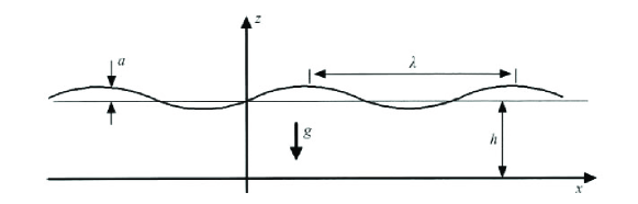
Figure 1: Water waves: general notations

Let $h$ be the mean level of the water and let $\eta(x,t)$ describes the shape of the water surface, i.e. the deviation from the average level. The pressure is $P(x,z,t)=P_{A}+\rho g(h-z)+p(x,z,t)$, where $P_{A}$ is the constant atmospheric pressure, and $p$ is a pressure variable, measuring the deviation from the hydrostatic pressure distribution.

On the surface $z=h+\eta$, $P=P_{A}$ and therefore $p=\eta\rho g$. Taking ${\bf v}\equiv(u,0,w)$ we can write the kinematic condition on the surface as $w=\eta_{t}+u\eta_{x}$ on $z=h+\eta$ [34]. Finally, there is no vertical velocity at the bottom, thus $w=0$ on $z=0$. All these equations can be written as a system

$$u_{t} + uu_{x}+wu_{z}=-\frac{1}{\rho}p_{x},$$

$$w_{t} + uw_{x}+ww_{z}=-\frac{1}{\rho}p_{z},$$

$$u_{x} + w_{z}=0,$$

$$w = \eta_{t}+u\eta_{x},\quad p=\eta\rho g\quad{\rm on}\quad z=h+\eta,$$

$$w = 0\quad{\rm on}\quad z=0.$$

Let us introduce now dimensionless parameters $\varepsilon=a/h$ and $\delta=h/\lambda$, where $a$ is the typical amplitude of the wave and $\lambda$ is the typical wavelength of the wave. Now we can introduce dimensionless quantities, according to the magnitude of the physical quantities, see [5, 34, 35] for details: $x\rightarrow\lambda x$, $z\rightarrow zh$, $t\rightarrow\frac{\lambda}{\sqrt{gh}}t$, $\eta\rightarrow a\eta$, $u\rightarrow\varepsilon\sqrt{gh}u$, $w\rightarrow\varepsilon\delta\sqrt{gh}w$, $p\rightarrow\varepsilon\rho gh$. This scaling is due to the observation that both $w$ and $p$ are proportional to $\varepsilon$ i.e. the wave amplitude, since at undisturbed surface ($\varepsilon=0$) both $w=0$ and $p=0$. The system in the new, dimensionless variables is

$$u_{t} + \varepsilon(uu_{x}+wu_{z})=-p_{x},$$

$$\delta^{2} ( w_{t}+\varepsilon(uw_{x}+ww_{z}))=-p_{z},$$

$$u_{x} + w_{z}=0,$$

$$w = \eta_{t}+\varepsilon u\eta_{x},\quad p=\eta\quad{\rm on}\quad z=1+\varepsilon\eta,$$

$$w = 0\quad{\rm on}\quad z=0.$$

3 Waves in the presence of shear

So far no assumptions have been made on the presence of shear. Now let us notice that there is an exact solution of the governing equations of the form $u=\tilde{U}(z)$, $0\leq z\leq h$, $w\equiv 0$, $p\equiv 0$, $\eta\equiv 0$. This solution represents an arbitrary underlying ’shear’ flow [6]. Let us consider waves in the presence of a shear flow. In such case the horizontal velocity of the flow will be $\tilde{U}(z)+u$. The scaling for such solution is clearly $u\rightarrow\sqrt{gh}\Big{(}\tilde{U}(z)+\varepsilon u\Big{)}$, where $u$ on the left-hand side is the horizontal velocity before the initial scaling, and the scaling for the other variables is as before. Thus, in this case we have (the prime denotes derivative with respect to $z$):

$$u_{t} + \tilde{U}u_{x}+w\tilde{U}^{\prime}+\varepsilon(uu_{x}+wu_{z})=-p_{x},$$ (1)

$$\delta^{2} ( w_{t}+\tilde{U}w_{x}+\varepsilon(uw_{x}+ww_{z}))=-p_{z},$$ (2)

$$u_{x} + w_{z}=0,$$ (3)

$$w = \eta_{t}+(\tilde{U}+\varepsilon u)\eta_{x},\quad p=\eta\quad{\rm on}\quad z=1+\varepsilon\eta$$ (4)

$$w = 0\quad{\rm on}\quad z=0.$$ (5)

We consider only the simplest nontrivial case: a linear shear, $\tilde{U}(z)=Az$, where $A$ is a constant ( $0\leq z\leq 1$). We choose $A>0$, so that the underlying flow is propagating in the positive direction of the $x$-coordinate. Burns condition [36] gives the following expression for $c$, the speed of the travelling waves in linear approximation :

$$c=\frac{1}{2}\Big{(}A\pm\sqrt{4+A^{2}}\Big{)}.$$ (6)

This expression will be derived again in our further considerations, e.g. see (15). Note that if there is no shear ($A=0$), then $c=\pm 1$.

Before the scaling the vorticity is $\omega=(U+u)_{z}-w_{x}$ or in terms of the rescaled variables ($\omega\rightarrow\sqrt{h/g}\phantom{*}\omega$),

$$\omega=A+\varepsilon(u_{z}-\delta^{2}w_{x}).$$

We are looking for a solution with constant vorticity $\omega=A$, and therefore we require that

$$u_{z}-\delta^{2}w_{x}=0.$$ (7)

This assumption amounts to considering approximate wave-solutions that are interactions of an underlying shear flow and an irrotational disturbance thereof. From (7), (3) and (5) we obtain

$$u = u_{0}-\delta^{2}\frac{z^{2}}{2}u_{0xx}+\mathcal{O}(\varepsilon^{2},\delta^{4},\varepsilon\delta^{2}),$$ (8)

$$w = -zu_{0x}+\delta^{2}\frac{z^{3}}{6}u_{0xxx}+\mathcal{O}(\varepsilon^{2},\delta^{4},\varepsilon\delta^{2}),$$ (9)

where $u_{0}(x,t)$ is the leading order approximation for $u$. Note that $u_{0}$ does not depend on $z$ since from (7) it follows that $u_{z}=0$ when $\delta\rightarrow 0$.

From (4) with (8) and (9) we obtain

$$\eta_{t}+A\eta_{x}+\Big{[}(1+\varepsilon\eta)u_{0}+\varepsilon\frac{A}{2}\eta^{2}\Big{]}_{x}-\delta^{2}\frac{1}{6}u_{0xxx}=0,$$ (10)

ignoring terms of order $\mathcal{O}(\varepsilon^{2},\delta^{4},\varepsilon\delta^{2})$.

From (2), (4), (8) and (9) we have (again, ignoring terms of order $\mathcal{O}(\varepsilon^{2},\delta^{4},\varepsilon\delta^{2})$)

$$p=\eta-\delta^{2}\Big{[}\frac{1-z^{2}}{2}u_{0xt}+\frac{1-z^{3}}{3}Au_{0xx}\Big{]}.$$

Then (1) gives (note that there is no $z$-dependence!)

$$\Big{(}u_{0}-\delta^{2}\frac{1}{2}u_{0xx}\Big{)}_{t}+\varepsilon u_{0}u_{0x}+\eta_{x}-\delta^{2}\frac{A}{3}u_{0xxx}=0.$$ (11)

Letting both the parameters $\varepsilon$ and $\delta$ to $0$, we obtain from (10), (11) the system of linear equations

$$u_{0t} + \eta_{x}=0,$$ (12)

$$\eta_{t} + A\eta_{x}+u_{0x}=0,$$ (13)

giving

$$\eta_{tt}+A\eta_{tx}-\eta_{xx}=0.$$ (14)

The linear equation (14) has a travelling wave solution $\eta=\eta(x-ct)$ with a velocity $c$ satisfying

$$c^{2}-Ac-1=0.$$ (15)

This gives the same solution for $c$ that follows from the Burns condition (6). There is one positive and one negative solution, representing left and right running waves. We assume that we have only one of these waves, then (e.g. from (12))

$$\eta=cu_{0}+\mathcal{O}(\varepsilon,\delta^{2}).$$ (16)

Let us introduce a new variable

$$\rho=1+\varepsilon\alpha\eta+\varepsilon^{2}\beta\eta^{2}+\varepsilon\delta^{2}\gamma u_{0xx},$$ (17)

for some constants $\alpha$, $\beta$ and $\gamma$. These constants will be determined in our further considerations. The variable $\rho$ will be used instead of $\eta$ as a tool for mathematical simplification of our equations. The expansion of $\rho^{2}$ in the same order of $\varepsilon$ and $\delta^{2}$ is

$$\rho^{2}=1+\varepsilon(2\alpha)\eta+\varepsilon^{2}(\alpha^{2}+2\beta)\eta^{2}+\varepsilon\delta^{2}(2\gamma)u_{0xx}.$$ (18)

With this definition one can express $\eta$ in terms of $\rho$ and write equation (10) in the form (keeping only terms of order $\mathcal{O}(\varepsilon,\delta^{2})$):

$$\frac{\rho_{t}+A\rho_{x}}{\alpha\varepsilon} + \delta^{2}\Big{(}\frac{\gamma}{\alpha}(c-A)-\frac{1}{6}\Big{)}u_{0xxx}$$ (19)

$$+ \Big{[}(1+\varepsilon\eta)u_{0}+\varepsilon\frac{A}{2}\eta^{2}+\varepsilon\frac{\beta}{\alpha}cu_{0}^{2}\Big{]}_{x}=0.$$

One can eliminate the $u_{0xxx}$-term by choosing

$$\frac{\gamma}{\alpha}=\frac{1}{6(c-A)}.$$ (20)

Equation (19) becomes

$$\frac{\rho_{t}+A\rho_{x}}{\alpha\varepsilon}+\Big{[}\Big{(}1+\varepsilon(1+\frac{Ac}{2}+\frac{\beta}{\alpha})\eta\Big{)}u_{0}\Big{]}_{x}=0.$$ (21)

With the choice

$$\alpha=1+\frac{Ac}{2}+\frac{\beta}{\alpha}$$ (22)

we can write (21) in the form

$$\rho_{t}+A\rho_{x}+\alpha\varepsilon(\rho u_{0})_{x}=0,$$ (23)

which contains only the variables $\rho$ and $u_{0}$ but not $\eta$.

4 Two component Camassa-Holm system

In this section we proceed with our derivation in a direction that leads to a two component Camassa-Holm system. Expressing $\eta$ in terms of $\rho$ in (11) we obtain (matching terms of order $\mathcal{O}(\varepsilon,\delta^{2})$):

$$m_{t}+Am_{x}-Au_{0x} + \delta^{2}\Big{(}\frac{A}{6}+\kappa(A-c)-\frac{\gamma}{\alpha}\Big{)}u_{0xxx}$$ (24)

$$+ \varepsilon\Big{(}1-\frac{\alpha^{2}+2\beta}{\alpha}c^{2}\Big{)}u_{0}u_{0x}+\frac{1}{2\varepsilon\alpha}(\rho^{2})_{x}=0,$$

where $m=u_{0}-\delta^{2}(\frac{1}{2}+\kappa)u_{0xx}$, $\kappa$ is arbitrary: we are adding and subtracting $\delta^{2}\kappa u_{0xxt}$, making use of (16). Fixing

$$\kappa=\frac{1}{A-c}\Big{(}\frac{\gamma}{\alpha}-\frac{A}{6}\Big{)}$$ (25)

leads to the disappearance of the $u_{0xxx}$ - term .

The relations (20) and (25) give

$$\kappa=\frac{1}{6(c-A)}\Big{(}A-\frac{1}{c-A}\Big{)}.$$ (26)

Thus equation (24) can be written as (matching only terms up to the order $\mathcal{O}(\varepsilon,\delta^{2})$)

$$m_{t}+Am_{x}-Au_{0x}+\varepsilon\frac{1}{3}\Big{(}1-\frac{\alpha^{2}+2\beta}{\alpha}c^{2}\Big{)}[2mu_{0x}+u_{0}m_{x}]+\frac{\rho\rho_{x}}{\varepsilon\alpha}=0.$$ (27)

Recall that $m=u_{0}-\delta^{2}Bu_{0xx}$, where (see (26) and (6))

$$B=\kappa+\frac{1}{2}=\frac{A^{2}-c^{2}+2}{3(c-A)^{2}}=\frac{1}{3c^{2}(c-A)^{2}}.$$ (28)

Note that $B$ is always positive and the denominator in (28) nonzero (since $c\neq A$ – see (15)). The rescaling $u_{0}\rightarrow\frac{1}{\alpha\varepsilon}u_{0}$, $x\rightarrow\frac{\delta}{\sqrt{B}}\phantom{*}x$, $t\rightarrow\frac{\delta}{\sqrt{B}}t$ in (27) and (23) is now only for the sake of mathematical clarity and simplicity and gives:

$$m_{t} + Am_{x}-Au_{0x}+\frac{1}{3\alpha}\Big{(}1-\frac{\alpha^{2}+2\beta}{\alpha}c^{2}\Big{)}[2mu_{0x}+u_{0}m_{x}]+\rho\rho_{x}=0,$$

$$m = u_{0}-u_{0xx},$$

$$\rho_{t} + A\rho_{x}+(\rho u_{0})_{x}=0.$$

Finally, we choose

$$\frac{1}{3\alpha}\Big{(}1-\frac{\alpha^{2}+2\beta}{\alpha}c^{2}\Big{)}=1$$ (29)

and thus

$$m_{t} + Am_{x}-Au_{0x}+2mu_{0x}+u_{0}m_{x}+\rho\rho_{x}=0,\quad m=u_{0}-u_{0xx},$$ (30)

$$\rho_{t} + A\rho_{x}+(\rho u_{0})_{x}=0.$$ (31)

The constants $\alpha$, $\beta$ and $\gamma$ can be determined from the constraints (22), (29) and (20):

$$\alpha = \frac{1}{3(1+c^{2})}+\frac{c^{2}}{3},$$ (32)

$$\beta = \Big{[}\frac{1}{3(1+c^{2})}-\frac{3+c^{2}}{6}\Big{]}\alpha,$$ (33)

$$\gamma = \frac{1}{6(c-A)}\alpha.$$ (34)

Note that from (32) it follows that $\alpha$ is always positive.

Now let us express the original variable $\eta$ in terms of the ’auxiliary’ variable $\rho$. Before the rescaling we had $\alpha\varepsilon\eta=\rho-1-\varepsilon^{2}\beta c^{2}u_{0}^{2}-\varepsilon\delta^{2}\gamma u_{0xx}$. Since in the leading order $\eta=cu_{0}$ the rescaling of $\eta$ is $\eta\rightarrow\frac{1}{\alpha\varepsilon}\eta$, thus in terms of the rescaled variables

$$\eta=\rho-1-\frac{\beta c^{2}}{\alpha^{2}}u_{0}^{2}-B\frac{\gamma}{\alpha}u_{0xx}.$$

With a Galilean transformation (that we use only to simplify our equations and to bring them to the form that is widely used), such that $\partial_{t^{\prime}}=\partial_{t}+A\partial_{x}$, $\partial_{x^{\prime}}=\partial_{x}$ ($x^{\prime}=x-At$, $t^{\prime}=t$) we obtain

$$m_{t^{\prime}} - Au_{0x^{\prime}}+2mu_{0x^{\prime}}+u_{0}m_{x^{\prime}}+\rho\rho_{x^{\prime}}=0,\quad m=u_{0}-u_{0x^{\prime}x^{\prime}}$$ (35)

$$\rho_{t^{\prime}} + (\rho u_{0})_{x^{\prime}}=0.$$ (36)

The system (35), (36) is an integrable 2-component Camassa-Holm system that appears in [28], generalizing the famous Camassa-Holm equation [1].

Let us drop the primes and write it in the form

$$m_{t} - Au_{0x}+2mu_{0x}+u_{0}m_{x}+\rho\rho_{x}=0,\quad m=u_{0}-u_{0xx}$$ (37)

$$\rho_{t} + (\rho u_{0})_{x}=0.$$ (38)

It generalizes the Camassa-Holm equation [1] in a sense that it can be obtained from it via the obvious reduction $\rho\equiv 0$. The system is integrable, since it can be written as a compatibility condition of two linear systems (Lax pair) with a spectral parameter $\zeta$:

$$\Psi_{xx}=\Big{(}-\zeta^{2}\rho^{2}+\zeta(m-\frac{A}{2})+\frac{1}{4}\Big{)}\Psi,\qquad\Psi_{t}=\Big{(}\frac{1}{2\zeta}-u_{0}\Big{)}\Psi_{x}+\frac{1}{2}u_{0x}\Psi.$$

The system is also bi-Hamiltonian. The first Poisson bracket is

$$\{F_{1},F_{2}\}=-\int\Big{[}\frac{\delta F_{1}}{\delta m}(-A\partial+m\partial+\partial m)\frac{\delta F_{2}}{\delta m}+\frac{\delta F_{1}}{\delta m}\rho\partial\frac{\delta F_{2}}{\delta\rho}+\frac{\delta F_{1}}{\delta\rho}\partial\rho\frac{\delta F_{2}}{\delta m}\Big{]}{\rm d}x$$

for the Hamiltonian $H_{1}=\frac{1}{2}\int(u_{0}(m-\frac{A}{2})+\rho^{2}){\rm d}x$.

The second Poisson bracket is

$$\{F_{1},F_{2}\}_{2}=-\int\Big{[}\frac{\delta F_{1}}{\delta m}(\partial-\partial^{3})\frac{\delta F_{2}}{\delta m}+\frac{\delta F_{1}}{\delta\rho}\partial\frac{\delta F_{2}}{\delta\rho}\Big{]}{\rm d}x$$

for the Hamiltonian $H_{2}=\frac{1}{2}\int(u_{0}\rho^{2}+u_{0}^{3}+u_{0}u_{0x}^{2}-Au_{0}^{2}){\rm d}x.$ It has two Casimirs: $\int\rho{\rm d}x$ and $\int m{\rm d}x$.

The system has an interesting interpretation in group-theoretical context. The first Poisson bracket gives rise to a Lie-algebraic structure. This fact is well studied in the case $\rho\equiv 0$ when the system coinsides with the Camassa-Holm equation [38, 39, 40, 41, 42]. Then the corresponding Lie algebra is the Virasoro algebra.

By considering the expansions

$$m=\frac{1}{2\pi}\sum_{n\in\mathbb{Z}}L_{n}e^{inx},\qquad\rho=\frac{1}{2\pi}\sum_{n\in\mathbb{Z}}\rho_{n}e^{inx}$$

we obtain the following Lie-algebra with respect of the first Poisson bracket:

$$i\{L_{n},L_{k}\} = (n-k)L_{n+k}-2\pi An\delta_{n+k},$$ (39)

$$i\{\rho_{n},L_{k}\} = n\rho_{n+k},$$ (40)

$$i\{\rho_{n},\rho_{k}\} = 0$$ (41)

The Lie algebra (39) – (41) is a semidirect product of the Virasoro algebra ($\mathfrak{vir}$) (39) with a central charge proportional to $A$, and the abelian algebra $C^{\infty}(\mathbb{R})$ (41) [37]. Note that the central extension of the Virasoro algebra contains only $An$ term but not $An^{3}$ term since the Hamilton operator contains only the first derivative $A\partial$. The system (37), (38) represents the equations of the geodesic motion on the corresponding Lie group $\mathfrak{Vir}\ltimes C^{\infty}(\mathbb{R})$ for the metric, defined by $H_{1}$:

$$||(u_{0},\rho)||^{2}=\int(u_{0}^{2}+u_{0x}^{2}+\rho^{2}){\rm d}x,$$

which is right-invariant under the natural group action.

5 Zakharov-Ito system

In this section we describe a derivation that matches the approximate equations (11), (23) (where $\rho$ is given in (17)) to the integrable Zahkarov-Ito system [29, 30, 43, 44]:

$$u_{0t} - 4ku_{0x}+u_{0xxx}+3u_{0}u_{0x}+\rho\rho_{x}=0.$$ (42)

$$\rho_{t} + (u_{0}\rho)_{x}=0,$$ (43)

where $k$ is an arbitrary constant. The system is formally integrable by the virtue of the Lax pair [45, 46]

$$\Psi_{xx}=\Big{(}\zeta-\frac{u_{0}}{2}+k-\zeta^{-1}\frac{\rho^{2}}{16}\Big{)}\Psi,\qquad\Psi_{t}=-(4\zeta+u_{0})\Psi_{x}+\frac{1}{2}u_{0x}\Psi.$$

Equation (11) can be written in the form (cf. (16) and (12))

$$u_{0t}+\delta^{2}Ku_{0xxx}+\varepsilon\Big{(}1-\frac{\alpha^{2}+2\beta}{\alpha}\Big{)}u_{0}u_{0x}+\frac{\rho\rho_{x}}{\alpha\varepsilon}=0.$$ (44)

where $K$ is a constant, given by [see (20) and (15)]

$$K=\frac{c}{2}-\frac{A}{3}-\frac{\gamma}{\alpha}=\frac{1}{3}(c-A).$$ (45)

For one of the roots of the equation in (6), $K$ is positive and for the other it is negative. We can fix the constants $\alpha$, $\beta$ and $\gamma$ by the conditions (22) and

$$\frac{1}{3\alpha}\Big{(}1-\frac{\alpha^{2}+2\beta}{\alpha}c^{2}\Big{)}=1,$$

which are formally the same as those for the Camassa-Holm system, giving the same expressions (32) – (34).

The rescaling $u_{0}\rightarrow\frac{1}{\alpha\varepsilon}u_{0}$, $x\rightarrow\frac{\delta}{\sqrt{K}}x$, $t\rightarrow\frac{\delta}{\sqrt{K}}t$ in (44) and (23) gives:

$$u_{0t} + Au_{0x}-Au_{0x}+u_{0xxx}+3u_{0}u_{0x}+\rho\rho_{x}=0,$$

$$\rho_{t} + A\rho_{x}+(\rho u_{0})_{x}=0.$$

Note that a coordinate change $(x,t)\rightarrow i(x,t)$ maps into another system with real variables and therefore if $K<0$ we still can apply formally the above rescaling. One can use a Galilean transformation $x^{\prime}=x-At$, $t^{\prime}=t$ to obtain

$$u_{0t^{\prime}} - Au_{0x^{\prime}}+u_{0x^{\prime}x^{\prime}x^{\prime}}+3u_{0}u_{0x^{\prime}}+\rho\rho_{x^{\prime}}=0,$$

$$\rho_{t^{\prime}} + (\rho u_{0})_{x^{\prime}}=0,$$

that matches the Zakharov-Ito system (42), (43) if the constant is chosen to be $k=A/4$. The ’physical’ variable $\eta$ in terms of the ’auxiliary’ $\rho$ and $u_{0}$ (for the rescaled variables) is

$$\eta=\rho-1-\frac{\beta c^{2}}{\alpha^{2}}u_{0}^{2}-K\frac{\gamma}{\alpha}u_{0xx}.$$

6 Kaup-Boussinesq system

Another integrable system matching the water waves asymptotic equations to the first order of the small parameters $\varepsilon,\delta$ is the Kaup-Boussinesq system [31, 33]. In this section we describe briefly its derivation. Introducing

$$V=u_{0}-\delta^{2}\Big{(}\frac{1}{2}-\frac{A}{3c}\Big{)}u_{0xx}\equiv u_{0}-\delta^{2}\Big{(}\frac{1}{6}+\frac{1}{3c^{2}}\Big{)}u_{0xx}$$

the equation (11) can be written as

$$V_{t}+\varepsilon VV_{x}+\eta_{x}=0.$$ (46)

Equation (10) in the first order in $\varepsilon,\delta^{2}$ is

$$\eta_{t}+\Big{[}A\eta+(1+\varepsilon\eta)u_{0}+\varepsilon\frac{A}{2}\eta^{2}\Big{]}_{x}-\delta^{2}\frac{1}{6}u_{0xxx}=0$$

and with a shift $\eta\rightarrow\eta-\frac{1}{\varepsilon}$ it becomes

$$\eta_{t}+\varepsilon(1+\frac{Ac}{2})(\eta u_{0})_{x}-\delta^{2}\frac{1}{6}u_{0xxx}=0,$$

or

$$\eta_{t}+\varepsilon\frac{1+c^{2}}{2}(\eta V)_{x}-\delta^{2}\frac{1}{6}V_{xxx}=0.$$ (47)

Further rescaling in (46) and (47) leads to the Kaup-Boussinesq system

$$V_{t}+VV_{x}+\eta_{x}=0,\qquad\eta_{t}-\frac{1}{4}V_{xxx}+\frac{1+c^{2}}{2}(\eta V)_{x}=0,$$

which is integrable iff $A=0$ ($c^{2}=1$) with a Lax pair

$$\Psi_{xx} = -\Big{(}(\zeta-\frac{1}{2}V)^{2}-\eta\Big{)}\Psi,$$

$$\Psi_{t} = -(\zeta+\frac{1}{2}V)\Psi_{x}+\frac{1}{4}V_{x}\Psi.$$

The integrability of the system, as well as the Inverse Scattering Method for it has been investigated firstly by D.J. Kaup [31]. His motivation has been to derive an integrable water-wave system with a second-order eigenvalue problem, which is readily solvable in comparison to the third-order eigenvalue problem for the Boussinesq equation. In our context, however, this system is relevant only in the case with zero vorticity.

7 Discussion

Apparently the described method can be used for other two-component integrable systems with a similar structure, e.g. see the classification in [46]. It is interesting to investigate further which specific properties of the original governing equations are preserved in the ’integrable’ approximate models. For example the 2-component Camassa-Holm system for certain initial data admits wave breaking [32]. Peakons do not occur in the case $A=0$ [32] and most certainly not in the case $A\neq 0$, due to the term with linear dispersion $Au_{0x}$. However, in the ’short-wave limit’ where $m=-u_{0xx}$ and $A=0$ peakon solutions are possible [32]. Recently a similar system with peakon solutions have been constructed in [47].

The case with $-\rho\rho_{x}$ term (instead of $+\rho\rho_{x}$) in (37) is also integrable [48] and it is studied in [49]. The two component Camassa-Holm system appears also in plasma theory models [50, 51] and in the theory of metamorphosis [52]. Other integrable multi-component generalizations of the Camassa-Holm equation (including other two-component ones) are constructed in [48].

References

- [1] R. Camassa and D.D. Holm, An integrable shallow water equation with peaked solitons, Phys. Rev. Lett. 71 (1993) 1661–1664; arXiv: patt-sol/9305002v1
- [2] A. Degasperis and M. Procesi, Asymptotic integrability. In: Symmetry and perturbation theory (ed. A. Degasperis and G. Gaeta), pp 23–37, Singapore: World Scientific: 1999.
- [3] A. Degasperis, D.D. Holm and A. Hone, A new integrable equation with peakon solutions, Theor. Math. Phys. 133 (2002) 1463–1474; arXiv: nlin/0205023v1 [nlin.SI]
- [4] H.R. Dullin, G.A. Gottwald and D.D. Holm, Camassa-Holm, Korteweg-de Vries-5 and other asymptotically equivalent equations for shallow water waves, Fluid Dynam. Res. 33 (2003) 73–95.
- [5] R.S. Johnson, Camassa-Holm, Korteweg-de Vries and related models for water waves, J. Fluid. Mech. 457 (2002) 63–82.
- [6] R.S. Johnson, The Camassa-Holm equation for water waves moving over a shear flow, Fluid Dyn. Res. 33 (2003) 97–111.
- [7] R.S. Johnson, The classical problem of water waves: a reservoir of integrable and nearly-integrable equations. J. Nonlinear Math. Phys. 10 (2003) suppl. 1, 72–92.
- [8] A. Constantin and D. Lannes, The hydrodynamical relevance of the Camassa-Holm and Degasperis-Procesi equations, Archive for Rational Mechanics and Analysis, 192 (2009) 165–186; arXiv: 0709.0905v1 [math.AP]
- [9] R.I. Ivanov, Water waves and integrability, Philos. Trans. R. Soc. Lond. Ser. A: Math. Phys. Eng. Sci. 365 (2007) 2267–2280; arXiv: 0707.1839v1 [nlin.SI]
- [10] A. Constantin and W. Strauss, Stability of peakons, Commun. Pure Appl. Math. 53 (2000) 603–610.
- [11] A. Constantin and J. Escher, Wave breaking for nonlinear nonlocal shallow water equations, Acta Mathematica, 181 (1998), 229–243.
- [12] H.P. McKean, Breakdown of the Camassa-Holm equation, Comm. Pure Appl. Math. 57 (2004) 416–418.
- [13] J. Escher, Y. Liu and Z. Yin, Shock waves and blow-up phenomena for the periodic Degasperis-Procesi equation, Indiana Univ. Math. J. 56 (2007) 87–117.
- [14] A. Constantin, On the blow-up of solutions of a periodic shallow water equation. J. Nonlinear Sci. 10 (2000) 391–399.
- [15] G. B. Whitham, Linear and nonlinear waves, J. Wiley and Sons Inc. (1999).
- [16] A. Constantin, Existence of permanent and breaking waves for a shallow water equation: a geometric approach, Ann. Inst. Fourier (Grenoble) 50 (2000) 321–362.
- [17] D. Henry, Persistence properties for the Degasperis-Procesi equation, J. Hyperbolic Differ. Eq. 5 (2008) 99–111.
- [18] A. Constantin, A Hamiltonian formulation for free surface water waves with non-vanishing vorticity, J. Nonlinear Math. Phys. 12 (2005) suppl. 1, 202–211.
- [19] A. Constantin, D. Sattinger, and W. Strauss, Variational formulations for steady water waves with vorticity, J. Fluid Mech. 548 (2006) 151–163.
- [20] A. Constantin, R.S. Johnson, Propagation of very long water waves, with vorticity, over variable depth, with applications to tsunamis. Fluid Dynam. Res. 40 (2008) 175–211.
- [21] A. Constantin, R.I. Ivanov and E.M. Prodanov, Nearly-Hamiltonian structure for water waves with constant vorticity, J. Math. Fluid Mech. 10 (2008) 224–237; arXiv: math-ph/0610014v1
- [22] A. Constantin, M. Ehrnström and E. Wahlén, Symmetry of steady periodic gravity water waves with vorticity, Duke Math. J. 140 (2007) 591–603.
- [23] E. Wahlén, A Hamiltonian formulation of water waves with constant vorticity, Lett. Math. Phys. 79 (2007) 303–315.
- [24] M. Groves and E. Wahlén, Small-amplitude Stokes and solitary gravity water waves with an arbitrary distribution of vorticity, Phys. D 237 (2008), 1530–1538.
- [25] M. Ehrnström, A new formulation of the water wave problem for Stokes waves of constant vorticity. J. Math. Anal. Appl. 339 (2008) 636–643.
- [26] V. Hur, Exact solitary water waves with vorticity. Arch. Ration. Mech. Anal. 188 (2008) 213–244.
- [27] J.-M. Vanden-Broeck, New families of steep solitary waves in water of finite depth with constant vorticity, European J. Mechanics. B Fluids 14 (1995) 761–774.
- [28] P. Olver and P. Rosenau, Tri-Hamiltonian duality between solitons and solitary-wave solutions having compact support, Phys. Rev. E 53 (1996) 1900.
- [29] V.E. Zakharov, The inverse scattering method, In: Solitons (Topics in Current Physics, vol 17) ed. R. K. Bullough and P. J. Caudrey (Berlin: Springer, 1980) pp 243–85.
- [30] M. Ito, Symmetries and conservation laws of a coupled nonlinear wave equation, Phys. Lett. A 91 (1982) 335–338.
- [31] D.J. Kaup, A higher-order water-wave equation and the method for solving it, Progr. Theoret. Phys. 54 (1975) 396–408.
- [32] A. Constantin and R. Ivanov, On an integrable two-component Camassa-Holm shallow water system, Phys. Lett. A 372 (2008) 7129–7132; arXiv: 0806.0868v2 [nlin.SI]
- [33] G.A. El, R.H.J. Grimshaw and M.V. Pavlov, Integrable shallow-water equations and undular bores. Stud. Appl. Math. 106 (2001) 157–186.
- [34] R.S. Johnson, A modern introduction to the mathematical theory of water waves, Cambridge: Cambridge University Press (1997).
- [35] A. Constantin, R.S. Johnson, On the non-dimensionalisation, scaling and resulting interpretation of the classical governing equations for water waves, J. Nonlinear Math. Phys. 15 (2008), suppl. 2, 58–73.
- [36] J.C. Burns, Long waves on running water, Proc. Cambridge Phil. Soc. 49 (1953) 695–706.
- [37] J. Hoppe, and the curvature of some infinite-dimensional manifolds, Phys. Lett. B 215 (1988) 706–710.
- [38] G. Misiolek, A shallow water equation as a geodesic flow on the Bott-Virasoro group, J. Geom. Phys. 24 (1998), 203–208.
- [39] D.D. Holm, J.E. Marsden and T.S. Ratiu, The Euler-Poincaré equations and semidirect products with applications to continuum theories, Adv. Math. 137 (1998) 1–81.
- [40] A. Constantin and B. Kolev, Geodesic flow on the diffeomorphism group of the circle, Comment. Math. Helv. 78 (2003) 787–804; arXiv: math-ph/0305013v1
- [41] A. Constantin and B. Kolev, Integrability of invariant metrics on the diffeomorphism group of the circle, J. Nonlin. Sci. 16 (2006) 109–122.
- [42] B. Kolev, Lie groups and mechanics: an introduction, J. Nonlinear Math. Phys. 11 (2004) 480–498; arXiv: math-ph/0402052v2
- [43] B.A. Kupershmidt, A coupled Korteweg de Vries equation with dispersion, J. Phys. A: Math. Gen. 18 (1985) L571–3,
- [44] M. Boiti, C. Laddomada, F. Pempinelli and G.Z. Tu, On a new hierarchy of Hamiltonian soliton equations, J. Math. Phys. 24 (1983) 2035–41.
- [45] N.N. Bogolyubov and A.K. Prikarpatskii, Complete integrability of the nonlinear Ito and Benney-Kaup systems: gradient algorithm and Lax representation, Theor. Math. Phys. 67 (1986) 586–96.
- [46] T. Tsuchida and T. Wolf, Classification of polynomial integrable systems of mixed scalar and vector evolution equations: I, J. Phys. A 38 (2005) 7691–7733; arXiv: nlin/0412003v2 [nlin.SI]
- [47] D.D. Holm, L. Ó Náraigh, C. Tronci, Singular solutions of a modified two-component Camassa-Holm equation, Phys. Rev. E 79, (2009) 016601; arXiv:0809.2538v1 [physics.flu-dyn].
- [48] R.I. Ivanov, Extended Camassa-Holm hierarchy and conserved quantities, Zeitschrift für Naturforschung 61a (2006) 133–138; arXiv:nlin/0601066v1 [nlin.SI].
- [49] J. Escher, O. Lechtenfeld and Z. Yin, Well-posedness and blow-up phenomena for the 2-component Camassa-Holm equation, Discrete Contin. Dyn. Syst. 19 (2007) 493–513.
- [50] J. Gibbons, D.D. Holm and C. Tronci, Vlasov moments, integrable systems and singular solutions. Phys. Lett. A 372 (2008) 1024–1033.
- [51] D.D. Holm and C. Tronci, The geodesic Vlasov equation and its integrable moment closures, Submitted to J. Geom. Mech , arXiv:0902.0734v1 [nlin.SI].
- [52] D.D. Holm, A. Trouve and L. Younes, The Euler-Poincaré theory of Metamorphosis, to appear in Quaterly of Applied Maths; arXiv: 0806.0870v1 [cs.CV].