The photometric evolution of dissolving star clusters

Abstract

Context. Evolutionary synthesis models are the prime method to construct spectrophotometric models of stellar populations, and to derive physical parameters from observations through comparison with such models. One of the basic assumptions for evolutionary synthesis models so far has been the time-independence of the stellar mass function (except for the successive removal of high-mass stars due to stellar evolution). However, dynamical simulations of star clusters in tidal fields have shown the mass function to change due to the preferential removal of low-mass stars from clusters.

Aims. Here we combine the results from dynamical simulations of star clusters in tidal fields (and especially the derived parametrisation of the changing mass function) with our evolutionary synthesis code GALEV to extend the models by a new dimension: the total cluster disruption time.

Methods. Following up on our earlier work, which was based on simplifying assumptions of the mass function time dependence, we reanalyse the mass function evolution found in N-body simulations of star clusters in tidal fields, parametrise it as a function of age and total disruption time of the cluster and use this parametrisation to compute GALEV models as a function of age, metallicity and the total cluster disruption time.

Results. We study the impact of cluster dissolution on the colour (generally, they become redder) and magnitude (they become fainter) evolution of star clusters, their mass-to-light ratios (which can deviate by a factor of $\sim$2 – 4 from predictions of standard models without cluster dissolution), and quantify the effect on the cluster age determination from integrated photometry (in most cases, clusters appear to be older than they are. Depending on the filter set available and the evolutionary stage of the cluster, the age difference can range from 20 to 200%). By comparing our model results with observed M/L ratios for old compact objects in the mass range 10^4.5 – 10⁸ M_⊙, we find a strong discrepancy for objects more massive than 10⁷ M_⊙, in a sense that observed M/L ratios are higher than predicted by our models. This could be either caused by differences in the underlying stellar mass function or be an indication for the presence of dark matter in these objects. Less massive objects are well represented by the models.
The models for a range of total cluster disruption times and metallicities are available online, at http://www.phys.uu.nl/$\sim$anders/data/SSP_varMF/ and http://data.galev.org, and will be made available via CDS.

1 Introduction

Since the pioneering work by Tinsley (Tinsley 1968; Tinsley & Gunn 1976; Tinsley 1980), evolutionary synthesis modelling has become the method-of-choice to predict spectrophotometric properties of stellar populations. Currently popular models include starburst99 (Leitherer et al. 1999), galaxev (Bruzual & Charlot 2003), galev (Anders & Fritze-v. Alvensleben 2003; Bicker et al. 2004), pegase (Fioc & Rocca-Volmerange 1997), and the Maraston models (Maraston 2005), all giving predictions for single-age populations , so-called “Simple Stellar Populations” (SSPs). In addition, galaxev, pegase and galev also provide models for populations with arbitrary extended star formation histories (SFH, like galaxies), while starburst99 only allows for an extended constant SFH. Comparing predictions from these models with observations allows to derive basic physical parameters of the studied system (e.g., among many others, Bicker et al. 2002; Kassin et al. 2003; Anders et al. 2004b; de Grijs et al. 2004; Kundu et al. 2005; de Grijs & Anders 2006; Smith et al. 2007).

While the specific input physics (e.g. the choice of stellar isochrones and spectral libraries, the inclusion of gaseous emission) and implementation varies among the models, some basic techniques and limitations are inherent to all of them: assigning a spectrum to each star along the isochrone, weighting them according to a chosen stellar initial mass function (IMF) and integrating along the isochrone (and over the SFH, if applicable) results in the integrated properties of the stellar population at a given age. For all currently available models, the stellar mass function (MF) is time-independently fixed at its initial value, the IMF.

Cluster disruption has become a well-studied phenomenon. It can be observed both in the earliest phases in a cluster’s life (the so-called “infant mortality” caused by the removal of gas left over from the cluster formation process by stellar winds and/or the first supernovae, see e.g. Lada & Lada 2003; Bastian & Goodwin 2006) and for old clusters (e.g. the prominent tidal tails of the Milky Way globular cluster Palomar 5, Odenkirchen et al. 2003). Age and mass distributions of a whole star cluster system can be used to determine the typical disruption time of clusters of a given mass in this cluster system (Boutloukos & Lamers 2003; Lamers et al. 2005b; Gieles et al. 2005). This cluster disruption time is predominantly determined by the external tidal field the cluster is experiencing (see Lamers et al. 2005b), the local density of giant molecular clouds (Gieles et al. 2006) and the occurrence of spiral arm passages (Gieles et al. 2007). In addition, the cluster loses mass due to stellar evolution. While in the case of “infant mortality” the cluster is likely (almost) completely disrupted (although a bound core might remain, see e.g. Bastian & Goodwin 2006 for “infant weight loss”), cluster dissolution in a smooth external tidal field is a more gradual process and accompanied by perpetual dynamical readjustment within the cluster. The latter is characterised by a mass-dependent probability to remove a star from a cluster: due to energy equipartition massive stars tend to sink towards the cluster center, while low-mass stars are driven outwards where they are more easily removed by the surrounding tidal field (Henon 1969; Spitzer & Shull 1975; Giersz & Heggie 1997). The resulting radial dependence of the mean stellar mass inside a cluster is called “mass segregation”. Mass segregation established by the very star formation process itself is referred to as “primordial mass segregation” (for observational evidence of “primordial mass segregation” see e.g. Gouliermis et al. 2004; Chen et al. 2007).

Baumgardt & Makino (2003) (from now on: BM03) performed the first (and, so far, most extensive) quantitative large-scale study of how the stellar MF inside a star cluster changes due to dynamical cluster evolution in a tidal field. They confirmed earlier findings for a preferential loss of low-mass stars and derived a formula describing the change in MF slope for low-mass stars. However, their derived formula (formula (13) in BM03) only applies to stars with masses $\leq$ 0.5 M_⊙, while the effect is pronounced also for higher-mass stars (see BM03 Fig. 7), which dominate the flux emerging from the cluster (for ages shorter than a Hubble time). BM03 performed their simulations for clusters not primordially mass-segregated. Recently, in Baumgardt et al. (2008), they studied also the dissolution of initially mass-segregated clusters (with a simplified initial setup different from the BM03 simulations, hence we can not combine these sets of simulations), finding an even stronger MF evolution than BM03. Marks et al. (2008) studied the evolution of the stellar MF inside star clusters during the gas removal/“infant weight loss” phase, and found it to also preferentially remove low-mass stars, leading to a flattening or even turning-over of the MF. This effect is most pronounced for initially mass-segregated clusters, and would be amplified by the later dynamical cluster evolution, as presented in BM03. Although their results can not be straightforwardly combined with the BM03 results (due to differences in model setups), both studies suggest even further enhancement of the effects studied in this paper.

In Lamers et al. (2006) we constructed simplified evolutionary synthesis models for solar metallicity, based on the galev models and the results from BM03. The main simplification made concerned the description of the changing (logarithmic) MF, which we modelled with fixed slopes, but a time-dependent lower mass limit (i.e. assuming that only the lowest-mass stars are removed from the cluster, while higher-mass stars might only be removed by stellar evolution). We scaled our models to match the total mass in stars with M $<$ 2 M_⊙ with the BM03 simulations.

Recently, this approach has been improved by Kruijssen & Lamers (2008) by incorporating the effects of stellar remnants for clusters of different initial masses and different total disruption times for a range of metallicities. They showed that the presence of stellar remnants plays a dominant role in the mass evolution of the clusters and therefore also in the evolution of the mass-to-light ratio. They also found that metallicity affects the colour evolution of the clusters, not only by the difference in the colours of the stars, but also by influencing the cluster dynamics due to the sensitivity of stellar mass and remnant formation on metallicity. They determined colours and mass-to-light ratios for a range of metallicities. Kruijssen (2008) compared these predicted mass-to-light ratios with the observed ones for cluster samples in different galaxies (Milky Way, Cen A, M31 and LMC) and found that the effects of mass segregation (and the associated preferential loss of low-mass stars) can explain the observed range much better than the range predicted by standard SSP models. As the models of Kruijssen & Lamers (2008) are based on the simplified assumption of only the lowest-mass stars being removed from the cluster, they can be improved by models in which the mass function changes in a physically more realistic manner, i.e. by changing the slope of the (logarithmic) mass function as derived from dynamical N-body simulations. This is the purpose of this paper.

We describe our input physics in Sect. 2, in particular we reanalyse the data presented in BM03 to derive formulae parametrising the changing mass function (Sect. 2.3). In Sect. 3 we present our new evolutionary synthesis models, and discuss the implications they have for mass-to-light (M/L) ratios and cluster age determinations from observations. In Sect. 4 we present a comparison with previous models (Lamers et al. 2006; Kruijssen & Lamers 2008) and investigate the impact of model uncertainties (fit uncertainties, initial-final mass relations, isochrones). We finish with our conclusions in Sect. 5.

2 Input physics

2.1 N-Body simulations by BM03

BM03 carried out a parameter study for dynamical evolution of clusters dissolving in a tidal field. They studied clusters with a range of particle numbers (8k – 128k, i.e. a range in cluster mass) on circular and elliptical orbits at different Galactocentric distances (i.e. strengths of the surrounding gravitational field). They accounted for mass lost due to stellar evolution (using fit formulae by Hurley et al. 2000), two-body relaxation and the external tidal field.

They initialised their clusters with a universal Kroupa (2001) IMF, which is of the form:

$$\xi(m){\rm d}m\sim\left\{\begin{array}[]{l l}m^{-1.3}{\rm d}m&\quad\mbox{$m<0.5{\rm M}_{\odot}$}\\ m^{-2.3}{\rm d}m&\quad\mbox{$m\geq 0.5{\rm M}_{\odot}$}\\ \end{array}\right.$$ (1)

with masses in the range $0.1{\rm M}_{\odot}\leq m\leq 15{\rm M}_{\odot}$. This rather low upper mass limit was chosen to account for the uncertain kick velocities of neutron stars (or equivalently, their ejection probability from the cluster, see BM03 for details).

The MFs provided by BM03 are for single stars, where dynamically created binaries are resolved in their components. They give the MF for the whole cluster (i.e. for all stars within the tidal radius). This MF compares well with the MF around the half-mass radius of the cluster, as shown by BM03.

BM03 do not take into account primordial mass segregation and primordial binaries. However, primordial mass segregation is found to even further increase the changes in the MFs found by BM03 (see Baumgardt et al. 2008). Primordial binaries seem to have little impact on the stars evaporating slowly from a cluster (see Küpper et al. 2008), but enhance the number of stars violently ejected during strong binary interactions. However, the latter are still only a small fraction of the stars leaving the cluster, hence we expect little changes in our conclusions if simulations with primordial binaries would have been included in our studies.

BM03 do not include a possibly present intermediate-mass black hole (IMBH) in the cluster. Recently, Gill et al. (2008) found that the presence of an IMBH reduces mass segregation in the centre, which might also influence the mass loss from star clusters, although this has still not been shown. In addition, the existence of IMBHs in star clusters is still under debate (see e.g. Maccarone & Servillat 2008).

2.2 Total cluster disruption time and the total cluster mass

Similar to BM03 we will identify the “total cluster disruption time” with the time when only 5% of the initial cluster mass remains bound. In order to avoid confusion, we will specifically label this time t_95%, i.e. the time when the cluster has lost 95% of its initial mass. However, we will provide our models for ages up to the point where a cluster with initially 10⁶ M_⊙ has lost all but 10² M_⊙ of its luminous mass (or to a maximum age of 16 Gyrs, whichever occurs first). This termination age of the cluster models is $\sim$ 20 – 26% longer than the cluster disruption time t_95% (for models with termination ages $<$ 16 Gyr, see Fig. 5, bottom panel).

As pioneered by Boutloukos & Lamers (2003) and Lamers et al. (2005b), we will use t₄ = t${}_{\rm dis}^{\rm total}(M=10^{4}M_{\odot}$), the total disruption time of a 10⁴ M_⊙ star cluster, as a rough proxy to characterise the strength of the gravitational field surrounding a cluster: the stronger the field the faster the cluster will dissolve, and the shorter t₄. Using the implicit equation

$$t_{\rm dis}^{\rm total}(M_{\rm i})=t_{4}\cdot\left(\frac{M_{\rm i}}{10^{4}M_{\odot}}\right)^{\gamma}\cdot\left(\frac{\mu_{\rm ev}(t_{\rm dis}^{\rm total})}{\mu_{\rm ev}(t_{4})}\right)^{\gamma}$$ (2)

for the total disruption time $t_{\rm dis}^{\rm total}$ (see Lamers et al. 2005a), t₄ can be translated into the total disruption time of clusters with arbitrary initial mass M_i. For example, a gravitational field characterised by t₄ = 1.3 Gyr (the value found by Lamers et al. 2005b for the Solar Neighbourhood) leads to complete disruption of a cluster with 10³ M_⊙ within approx. 300 Myr, while a 10⁶ M_⊙ cluster would survive for 22.6 Gyr. $\mu_{\rm ev}(t)$ describes the fraction of the mass that the cluster would have at time $t$ if stellar evolution was the only mass loss mechanism, and $\gamma$=0.62 (as determined from observations by Boutloukos & Lamers 2003; Lamers et al. 2005b, and in agreement with N-body simulations, see BM03 and Gieles & Baumgardt 2008).

The total cluster mass as a function of the fractional age t/t_95% is derived from formula (6) in Lamers et al. (2005a) (who also show the good agreement with the data from BM03):

$$M_{\rm tot}(t)=M_{\rm i}\cdot\left\{\mu_{\rm ev}(t)^{\gamma}-\frac{t}{t_{\rm 95\%}}\cdot\left[\mu_{\rm ev}(t_{\rm 95\%})^{\gamma}-0.05^{\gamma}\right]\right\}^{1/\gamma}$$ (3)

with $M_{\rm i}$ = 10⁶ M_⊙ the initial cluster mass. The stellar evolution part of this equation was taken directly from the galev models used in the remainder of this work (for details see below).

Since the total disruption time of clusters in a given environment (e.g. tidal field) depends on the initial cluster mass, Eq. 3 can also be used to calculate the initial cluster mass for an observed present-day total mass and adopted t_95%.

The mass fraction in stellar remnants is taken from BM03 (their formula (16)):

$$f_{\rm rem}(t)=f^{\rm se}_{\rm rem}(t)+0.18\cdot\left(\frac{t}{t_{\rm 95\%}}\right)^{2}+0.16\cdot\left(\frac{t}{t_{\rm 95\%}}\right)^{3}$$ (4)

with $f^{\rm se}_{\rm rem}$ the mass fraction in stellar remnants from stellar evolution only (i.e. without dynamical cluster evolution effects) taken from our galev models, and the other two terms describe the increase in the mass fraction of the remnants due to the preferential loss of low-mass non-remnant stars.

The luminous mass is then:

$$M_{\rm lum}(t)=M_{\rm tot}(t)\cdot(1-f_{\rm rem}(t)).$$ (5)

2.3 Parametrising the changing mass function

Throughout the paper we look at the logarithm of the logarithmically binned mass function (MF). Hence, for a Salpeter (1955) MF, the power-law index -2.35 becomes a linear slope of -1.35.

In order to parametrise the changes in the (logarithmic) mass function, we

• took the MF data from BM03

• divided them by the IMF (by doing so we remove the power law break at 0.5 M_⊙ of the Kroupa 2001 IMF)

• skipped the 2 highest not-empty mass bins (as those are affected and partially emptied by stellar evolution), and

• fitted the remainder with a piecewise power law, independently for every simulation and age.

We tried fitting slopes and break points simultaneously, finding the results for the break points scattering in the range 0.25 – 0.35 M_⊙. This scatter was found to be uncorrelated with any other quantity, confirming it to be of random nature. Hence, we chose a double power-law with a break point fixed to 0.3 M_⊙, and only fitted the slopes below and above this break point independently for every simulation and age. In Fig. 1 we show the slopes of the changing MF, relative to the slopes of the IMF (i.e. $\alpha(t)-\alpha(0)$). The points are derived by fitting the data from BM03, using the abovementioned scheme, and then the median in bins of $\Delta(t/t_{\rm 95\%})$ = 0.025 was taken. The error bars represent the 16% and 84% percentiles of individual data points in each bin, equivalent to 1$\sigma$ ranges for a Gaussian distribution. These data are grouped according to their disruption time t_95%: t_95% $\leq$ 3.5 Gyr = filled orange diamonds, 3.5 Gyr $<$ t_95% $\leq$ 6 Gyr = open blue triangles, 6 Gyr $<$ t_95% $\leq$ 10 Gyr = filled green circles, and 10 Gyr $<$ t_95% = open black squares.

This fit formula, in conjunction with the Kroupa (2001) IMF, leads to a 3-component power-law MF with break points at 0.3 M_⊙ and 0.5 M_⊙ and time-dependent slopes.

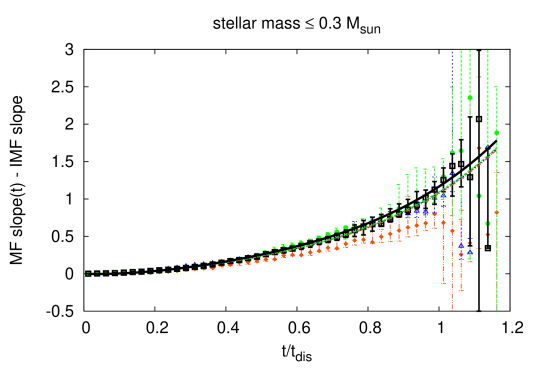
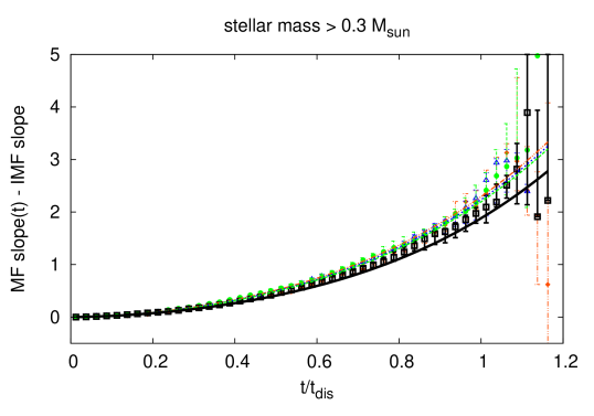
Figure 1: Dependence of MF slopes (top panel: for stellar masses $\leq$ 0.3 M_⊙, bottom panel: for stellar masses $>$ 0.3 M_⊙) on the fractional age t/t_95%. Symbols represent median slopes (and 16% and 84% percentiles uncertainty ranges) derived from individual data from BM03 runs, and binned in intervals of $\Delta(t/t_{\rm 95\%})$ = 0.025. The data are grouped according to their disruption times: t_95% $\leq$ 3.5 Gyr (filled orange diamonds), 3.5 Gyr $<$ t_95% $\leq$ 6 Gyr (open blue triangles), 6 Gyr $<$ t_95% $\leq$ 10 Gyr (filled green circles), 10 Gyr $<$ t_95% (open black squares). Smooth lines represent the fit formula (6) for the respective age ranges: t_95% = 1 Gyr (orange dot-dot-dashed line), 5 Gyr (blue, dotted), 8 Gyr (green, dashed) and 30 Gyr (black, solid). Shown is the difference between the time-dependent slope of the MF and the slope of the IMF (i.e. $\alpha(t)-\alpha(0)$).

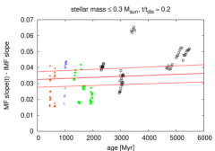
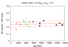
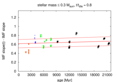
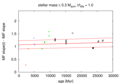
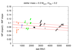
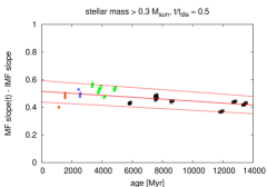
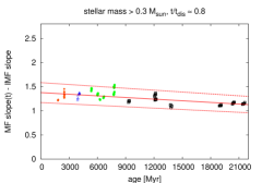
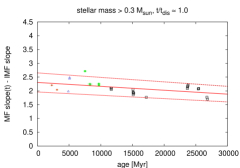
Figure 2: Dependence of MF slope on the age (in Myr) of the cluster for stellar masses $\leq$ 0.3 M_⊙ and for 4 different fractional ages t/t_95%: t/t_95% = 0.15-0.25 (top left panel), t/t_95% = 0.45-0.55 (top right), t/t_95% = 0.75-0.85 (bottom left), and t/t_95% = 0.95-1.05 (bottom right). In each panel, the solid line represents the fit formula (6) for the appropriate t/t_95%, the dashed lines represent the median spread ranges (85% and 115% of fit line). Points are the same as Fig. 1. Please beware of the very different vertical axes. The y-axes are chosen to go from 0 to 2$\times$maximum fit value.

Figure 3: Same as Fig. 3, but for stellar masses $>$ 0.3 M_⊙.

The time evolution of the changing MF slopes can be expressed as:

$$\begin{array}[]{l l}\alpha(t)=&\alpha_{\rm IMF}(0)\\ &+a_{1}\cdot x+a_{2}\cdot x^{2}+a_{3}\cdot x^{3}+a_{4}\cdot x^{4}\\ &+b\cdot x\cdot t\end{array}$$ (6)

where “t” is the cluster age in Myrs, while “x” = t/t_95% is the fractional cluster age in units of its total disruption time. The best-fit coefficients are provided in Table 1. These fit parameters have a very high formal accuracy, due to the large number of data points used for the fit. However, the spread of N-body models around our best fit is the dominant source of uncertainty (see below and Sect. 4.1). We therefore omit the formal fit uncertainties in Table 1.

In Fig. 1 we overplot our fit formulae for 4 disruption times t_95% (1 Gyr, 5 Gyr, 8 Gyr and 30 Gyr), representative for the chosen grouping in disruption time.

We restrict the fitting to ages $\leq$ t_95%, as in many cases clusters with larger ages do not contain enough stars to determine the MF slopes with reasonable accuracy. However, the general trends continue beyond t_95%, following the fitted relation further on, allowing an extrapolation for ages $>$ t_95% (see Fig. 1).

In addition, we take only simulations into account which started with 32k or more particles (these simulations have total disruption times in the range 2.3 – 25.5 Gyr), as many simulations with lower particle numbers show substantial uncertainties in the determined MF slopes.

We would like to emphasize that considering all simulations with 16k or more particles or with 64k or more particles yield fitted slopes which deviate from the 32k results only by less than $\pm$ 0.1 for ages up to at least 1.3 $\times$ t_95%. Considering also 8k simulations or only the 128k simulations yields larger deviations, due to large run-to-run scatter and small number of data/coverage of parameter space, respectively.

On average, the spread of the BM03 simulation results around the fitted relation Eq. 6 is of the order of 15%, as shown in Fig. 3 and 3. For ages $\la$ 1/3 $\times$ t_95% these relative deviations are larger, however, at those times the absolute deviations of the data from the fit formulae are small (of the order of $\Delta$slope = 0.02-0.03). The impact of this uncertainty will be further discussed in Sect. 4.1.

Although the BM03 simulations are performed for a metallicity Z=0.001 (using the fitting formulae from Hurley et al. 2000), we will use Eq. 6 for all metallicities, assuming the metallicity to – at most – introduce second-order effects on cluster dynamics. This is supported by Hurley et al. (2004), who find metallicity effects largely cancelling each other, resulting in a weak overall metallicity dependence of cluster dynamics (although details are metallicity-sensitive).

Table 1: The best-fit coefficients for Eq. (6). The middle column gives the coefficients for the low-mass end of the MF, for masses $\leq$ 0.3 M_⊙. The right column gives the coefficients for masses $>$ 0.3 M_⊙.

coefficient	m $\leq$ 0.3 M⊙	m $>$ 0.3 M⊙
$a_{1}$	-0.1345	0.08389
$a_{2}$	1.7986	1.9324
$a_{3}$	-1.8121	-0.4435
$a_{4}$	1.2181	0.734
$b$	3.215e-6	-1.4143e-5

2.4 The galev models

The galev models are extensively described in Schulz et al. (2002), Anders & Fritze-v. Alvensleben (2003) and Bicker et al. (2004). Here we give only a brief summary of the relevant input physics used.

The galev models used in this work are based on isochrones from the Padova group, first presented in Bertelli et al. (1994), and subsequently updated to include the TP-AGB phase. This update, although not documented in a refereed publication, was made publicly available approx. 1999, and treats the TP-AGB phase as later described in Girardi et al. (2000). As we will mainly concentrate on the evolution of old stellar clusters, the Padova isochrones are preferred over the Geneva isochrones (Schaller et al. 1992). We want to emphasise (and stimulate the various groups of stellar evolution modellers) that the isochrone sets by Bertelli et al. (1994) and Schaller et al. (1992) (and associated papers) are the only available isochrones which cover stellar evolution (in a consistent way) up to its final stages as well as a mass range up to $\sim$ 120 M_⊙ required to correctly model ongoing star formation in galaxies. For further discussion of this point see Sect. 4.3.

For consistency with the BM03 simulations we use a Kroupa (2001) IMF.

At each age, the time-dependent MF is evaluated from equation (6) for the requested total disruption time t_95%. To each star from the isochrones an appropriate spectrum from the BaSeL library (Lejeune et al. 1997, 1998) and a weight according to the time-dependent MF are assigned. Then the integrated spectra is obtained by summing up the contributions from the individual stars. Here, we assume a well-populated MF, hence any stochastic effects due to small number statistics, especially at the high-mass end of the MF, are neglected. Hence, we model an average star cluster.

The treatment of stochastic effects would go well beyond the scope of this paper. The impact of such stochastic effects was studied in depth by Cerviño and collaborators (see e.g. Cerviño & Mollá 2002; Cerviño & Luridiana 2004, 2006) and Fagiolini et al. (2007), who found these effects to be strongly age- and wavelength-dependent. The strongest impact is found for red passbands, which are dominated by few red supergiants (young clusters) or very bright upper RGB and AGB stars (intermediate-age clusters). The effects become smaller for older ages, for non-dissolving clusters. However, the decreasing number of stars with age in our dissolving cluster models likely counteracts this effects. We therefore caution users about applying our models to a single cluster. The models represent average star clusters with the given parameters, hence need to be applied to a whole star cluster system.

More generally, small number statistics is the likely origin of the scatter seen in Figs. 3 and 3. However, as we use 19 BM03 models with a variety of parameters (i.e. total masses and dissolution times) to model the dissolution we can describe the average cluster dissolution. The impact of the spread seen in Figs. 3 and 3 will be discussed in more detail in Sect. 4.1.

Due to computational restrictions we only calculated individual models for MF slopes with 2 decimal places. If at any given age the MF slopes were identical to within these 2 decimal places with the MF slopes of a previously computed model we reused this older model. Due to this finite step-size, some cluster colours exhibit small jumps of the order of $\sim$0.001 mag (up to 0.004 mag for the most extreme cases).

The spectrophotometry is normalised to a luminous cluster mass as described in Sect. 2.2.

We calculate models for t_95%:

• in the range of 100 – 900 Myr: in 50 Myr steps

• in the range of 1 – 16 Gyr: in 500 Myr steps

• for t_95% = 18, 20, 25, 30, 40, 60, 100, 150 and 200 Gyr

and for metallicities (limited by the metallicities provided by the Padova isochrones):

• Z=0.0004 $\leftrightarrow$ [Fe/H] = – 1.7

• Z=0.004 $\leftrightarrow$ [Fe/H] = – 0.7

• Z=0.008 $\leftrightarrow$ [Fe/H] = – 0.4

• Z=0.02=Z_⊙ $\leftrightarrow$ [Fe/H] = 0.0

• Z=0.05 $\leftrightarrow$ [Fe/H] = + 0.4

For t${}_{\rm 95\%}\mathrel{\hbox to0.0pt{\lower 3.0pt\hbox{$\mathchar 536\relax$}\hss}\raise 2.0pt\hbox{$\mathchar 318\relax$}}$ 200 Gyr, within a Hubble time the MF slopes deviate from the universal Kroupa (2001) IMF by less than 0.005. For conditions similar to the Solar Neighbourhood, i.e. t₄ = 1.3 Gyr as determined by Lamers et al. 2005b, the range in total disruption times corresponds to a cluster mass range 160 – $3.4\times 10^{7}$ M_⊙ (i.e. a 160 M_⊙ cluster needs 100 Myr to totally disrupt, a 10⁴ M_⊙ cluster needs 1.3 Gyr, and a $3.4\times 10^{7}$ M_⊙ cluster needs 200 Gyr). For the SMC, with t₄ = $\sim$10 Gyr, the range in total disruption times would correspond to a cluster mass range 6 – $1.25\times 10^{6}$ M_⊙.

The data are made publicly available at our webpages http://www.phys.uu.nl/$\sim$anders/data/SSP_varMF and http://data.galev.org. We provide the user with integrated cluster magnitudes in a variety of passbands plus cluster masses (total mass, luminous mass and mass in stellar remnants) for each of the models. Integrated spectra are available upon request.

3 Results and implications

In this section we present our new models for solar metallicity (unless otherwise noted) and discuss its implications. Models for all metallicities are available at our webpages http://www.phys.uu.nl/$\sim$anders/data/SSP_varMF and http://data.galev.org. We would like to emphasize that the absolute values of our models (and therefore also the results and implications discussed in this section) depend on our choice of isochrones and other input physics. In Sect. 4 we discuss some of these uncertainties. The main results, the systematic differences induced by the preferential mass loss, are hardly changed.

3.1 Photometry

The photometry for the new models is shown in Fig. 4. The colours are shown as differences between the new models with changing MF and the standard models with fixed (initial) MF. For illustrative purposes, in the bottom left panel the absolute values for the V-I colour are presented. The V-band magnitude evolution (bottom right panel) is given in absolute values for a 10⁶ M_⊙ cluster.

The V-band magnitude evolution shows the stellar evolution fading line as bright limit for the new models, which they follow for young ages, when the effect of mass loss is not yet pronounced. Already after $\sim$10% of their respective total disruption times, the new models have evolved 0.1 mag away from the fiducial fading line, due to the loss of stars. At $\sim$80% ($\pm$ 10%, depending on the model) of their respective total disruption times, the new models are 1 mag fainter than standard models predict, due to the loss of stars.

Except for the very earliest stages of cluster evolution (first few Myrs), the flux in passbands redder than the V band is dominated by stars initially more massive than the main contributors to the flux in bluer passbands. This is caused by the flux in the red passbands being dominated by red (super)giants, which are more luminous than the stars at the low-mass end of the main sequence (MS), even after taking the larger number of low-mass MS stars due to the IMF into account. For a changing MF due to dynamical evolution, the contribution from low-mass MS stars is even further reduced.

The dominant source of flux contribution in passbands including and bluewards of the V band is a strong function of time: in early stages, the flux is dominated by mid-MS stars (the evolution through the Hertzsprung gap is too fast to significantly contribute). As the cluster ages, the MS turn-off (MSTO) shifts successively redwards through the filters, ever increasing its contribution to the band’s flux. However, the relative contribution of mid-MS stars and MSTO stars is also strongly dependent on the MF, hence is dependent on the total disruption time of our models.

As the selective mass loss preferentially removes the least massive stars from the cluster (and therefore its integrated photometry), it causes the cluster to generally become redder than the standard models without cluster dissolution (i.e. with infinite total cluster disruption time). The MF evolution and the resulting reddening speeds up while the cluster approaches its final disruption, leading to the steep colour evolutions towards the end of a cluster’s lifetime, as seen in Fig. 4.

Two exceptions have to be noted:

• the colour U-B (and similar colours) becomes bluer than the standard models for total disruption times shorter than $\sim$ 1Gyr. At these ages the B band is entirely dominated by mid-MS stars, while bluer bands contain contributions from the higher MS stars and the MSTO stars. As the mid-MS is stronger depopulated than the upper MS and MSTO due to the dynamical cluster evolution, the colours become bluer. For longer total disruption times the mid-MS is not sufficiently depopulated to notice the effect until the B band gets contributions from the MSTO stars. Redder passbands do not show this effect as they contain contributions from bright red (super-)giants.

• for colours like V-R and V-I and ages $\ga$ 6 Gyr the models get slightly bluer than the standard models for total disruption times $\ga$ 10 Gyr. Likely, this comes from the strong depopulation of the lower MS (and the standard IMF containing a large number of stars at low masses), which leaves an imprint even though a single lower-MS star is 3-4 mag fainter than an RGB/AGB star of similar temperature. Redder passbands do not show this effect as the magnitude difference between lower-MS stars and RGB/AGB stars increases with increasing wavelength/decreasing temperature, and the total contribution from MS stars decreases.

For long total disruption times, the maximum colour deviation of our models for dissolving clusters from the standard models decreases with increasing total disruption time. This comes from several effects at once:

• for such old ages, the MF covers only a narrow mass range in both cases

• the integrated cluster flux is dominated by the upper-RGB/AGB stars, as they are significantly brighter than the MSTO region (the magnitude difference between upper-RGB/AGB and MSTO increases with time), resulting in an even narrower “effectively visible MF” range

• the temperature range these stars cover is significantly smaller than at younger ages, resulting in a lower sensitivity of the colours to the exact distributions of stars along the isochrone.

However, the changes in mass/absolute magnitude (see Fig. 4, bottom right panel) and M/L ratio (see next section) are significant in all cases.

The increasing maximum colour deviation of our dissolving clusters models from the standard models for blue passbands and increasing total disruption times $\mathrel{\hbox to0.0pt{\lower 3.0pt\hbox{$\mathchar 536\relax$}\hss}\raise 2.0pt\hbox{$\mathchar 316\relax$}}$ 1 Gyr originates from the redward shifting of the MSTO through the filters.

Figure 4: Solar metallicity models with the changing mass function treatment, following equation (6) with t_95% in the range 100 Myr – 100 Gyr (for clarity only models at 100, 200, 400, 800 Myr and 1, 2, 4, 8, 10, 12, 14, 16, 18, 20, 40, 100 Gyr are shown), going from left to right, respectively. Upper left panel: U-B colour, top right: B-V, middle left: V-I, middle right: V-K. For these colours, the differences between the new models and the standard models are displayed. Bottom left: the absolute values for V-I, bottom right: V-band magnitude evolution of a 10⁶ M_⊙ cluster. Thick lines represent the standard models.

3.2 Mass-to-light ratios

The low-mass stars preferentially removed in the course of cluster dissolution have mass-to-light (M/L) ratios which are higher than the M/L ratio of the average cluster star. On the other hand, as shown by BM03, the fraction of (non-luminous) stellar remnants in dissolving clusters is enhanced w.r.t. the standard models. These effects partially cancel each other and lead to the time-dependent M/L ratios shown in Fig. 5. It demonstrates that for each total disruption time the M/L ratio of our dissolving cluster models is systematically lower than a standard model would suggest for the majority of a cluster’s total disruption time. For the final up to $\sim$16% of a cluster’s total disruption time, the M/L ratio can become enhanced w.r.t. the standard models (see Fig. 5, bottom panel). This is caused by the increasing fraction of stellar remnants inside the cluster.

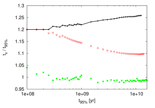
Figure 5: Same models as Fig. 4, but M/L ratios. Upper panel: time evolution of V-band M/L ratio for the new models. Middle panel: ratio of new model’s V-band M/L ratio and V-band M/L ratio from standard models. The non-dissolving/standard model is shown as thick line. Bottom panel: characteristic times of the models as function of total disruption time: black crosses and line = age at which the cluster contains only 100 M_⊙ luminous matter (i.e. termination age of model); red open circles = age at which the M/L ratio evolution crosses the standard model; green filled squares = age at which the M/L ratio of the dissolving cluster models is minimal w.r.t. the standard models (i.e. the dip seen in the middle panel). Only models for which the respective age is smaller than the maximum model age of 16 Gyr are shown.

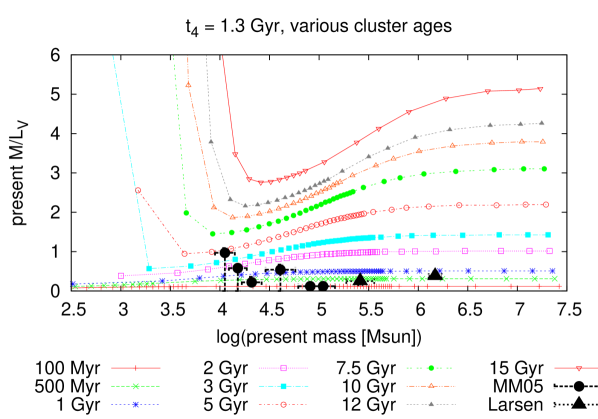
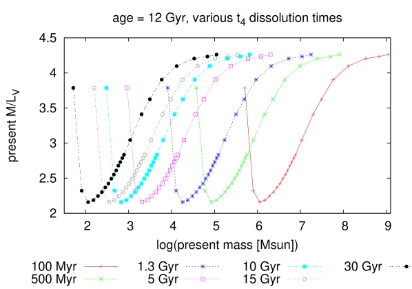
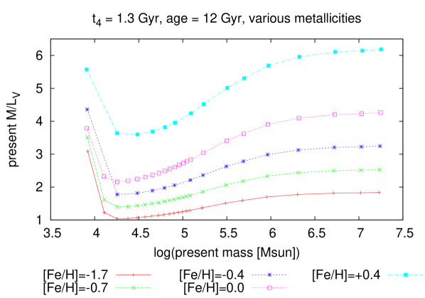
Figure 6: Top panel: time evolution of V-band M/L ratio (for solar metallicity) as a function of present-day cluster mass for a fixed local gravitational field strength characteristic for the Solar Neighbourhood (i.e. t₄=1.3 Gyr, see Lamers et al. 2005a). Middle panel: V-band M/L ratio (for solar metallicity) as a function of present-day cluster mass for a range of local gravitational field strengths for clusters observed at an age of 12 Gyr. Bottom panel: V-band M/L ratio as a function of present-day cluster mass for a range in metallicity for clusters observed at an age of 12 Gyr and experiencing a typical disruption time t₄=1.3 Gyr. In the top panel, observations from McLaughlin & van der Marel (2005) (MM05) and from Larsen & Richtler 2004; Larsen et al. 2004 are overplotted, for young clusters with ages $<$ 1 Gyr.

In Fig. 6 we present the dependence of the V-band M/L ratio on the present cluster mass. The top panel shows how this relation evolves with cluster age at a field strength (i.e. location in a galaxy, characterised by t₄, the total disruption time of a 10⁴ M_⊙ cluster, as described in Sect. 2.2) representative for the Solar Neighbourhood, as found by Lamers et al. (2005a). As the clusters evolve, generally the M/L ratio increases due to stellar evolution. In addition, the lowest-mass clusters eventually disrupt (and drop out of this plot). The highest-mass clusters lose mass, but still have M/L ratios close to the canonical value from stellar evolution. Intermediate-mass clusters suffer from the impact of the changing mass function which reduces their M/L ratio significantly compared to the canonical value. A few cases of enhanced M/L ratios can be seen for clusters close to final disruption (at the low-mass end of the curves).

In Fig. 6 (top panel) we overplotted data of young (ages $<$ 1 Gyr) LMC and SMC clusters by McLaughlin & van der Marel (2005) (labelled “MM05”, for details of this dataset see following subsection) and Larsen and collaborators (labelled “Larsen”) in 4 spiral and irregular galaxies, (see Larsen & Richtler 2004 and Larsen et al. 2004). Out of the 13 clusters in these samples, 8 have M/L ratios consistent with our models for their respective ages (within their 1$\sigma$ uncertainty ranges). The remaining 5 clusters all have too high M/L ratios for their respective ages. 2 clusters are very young ($\sim$10 Myr), hence could be out of equilibrium during their gas expulsion and readjustment phase, and their velocity dispersions might not trace their dynamical masses (see Goodwin & Bastian 2006). The deviations of the remaining clusters might be indications of errors in the models, or could be signs that the age determination is uncertain or the velocity dispersions are seriously affected by the orbital motions of binaries (or other systematic observational effects, like macroturbulence in the stellar atmospheres or instrumental resolution).

The middle panel shows the M/L ratio in the V band as a function of the present-day mass of 12 Gyr old clusters, for a range of gravitational field strengths (i.e. typical disruption times t₄). Within each line, the cluster’s total disruption time goes from 10 Gyr (low mass end; clusters with shorter total disruption times have been disrupted by an age of 12 Gyr) to 200 Gyr (upper end of available total disruption time range). For example: a cluster located at a position in a galaxy characterised by a field strength with t₄ = 1.3 Gyr (i.e. the blue line, corresponding to the environment in the Solar Neighbourhood), observed now (i.e. at an age of 12 Gyr) with a mass = 10⁶ M_⊙ is expected to have a M/L_V of $\sim$4, while a cluster with a mass = 10⁴ M_⊙ has a modelled M/L_V of $\sim$2.3.

The bottom panel shows the impact of metallicity on the M/L ratios: with increasing metallicity the M/L_V ratio based on stellar evolution increases. Therefore all curves are stretched to reach higher M/L_V ratios for higher metallicities, while the shape of the curves is largely unaffected. At the high-mass end, all curves level off to their respective values determined by stellar evolution alone.

By comparing the top and bottom panels of Fig. 6, both for our new models as for the non-dissolving standard models the well-known age-metallicity degeneracy is apparent (see e.g. Worthey 1994).

As the galev code (like most other evolutionary synthesis codes) is not capable to directly deal with stochastic effects (especially not with the stochastic effects inherent to the selective mass loss caused by dissolution), we employ the following estimation scheme:

• We assume, that the majority of stochasticity originates from evolved stars (mainly RGB, AGB stars).

• As a function of age, we determine the relative number of evolved to unevolved stars (i.e. MS stars).

• From this relative number we determine the total number of evolved stars for clusters of different masses, and the stochastic scatter (i.e. the square root of the total number of evolved stars).

• We determine average properties of the evolved stars (mean effective temperature, mean log(g) and mean luminosity).

• We multiply the stochastic scatter with the spectrum of the mean evolved star, and add resp. subtract this from our standard spectrum.

From this approach, we estimate the effect of IMF stochasticity on the M/L ratios to be roughly: 15/5/1.5 % uncertainty for clusters with total mass 10,000/100,000/1,000,000 M_⊙, respectively. This test was only done for the standard, not depopulated IMF. The effects for the depopulated MF will be smaller, as for the same total mass, the number of giant stars will be larger.

Our results show features similar to those presented by Kruijssen & Lamers (2008) and applied by Kruijssen (2008). However, systematic differences are present, inherent to the underlying assumptions, and discussed in Sect. 4.4.

3.2.1 Comparison with observations

In the following section we want to compare our new models with old globular clusters (and other old massive stellar systems) in the Milky Way and other galaxies. This is a first step to validate our models.

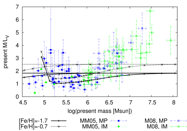
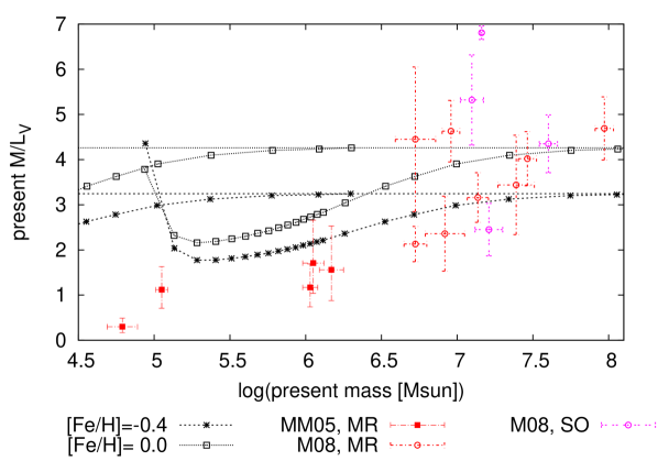
Figure 7: Observations of old ($\sim$12 Gyr) objects from McLaughlin & van der Marel (2005) (MM05) and Mieske et al. 2008 (M08). Top panel: objects with [Fe/H] $<$ -0.55. Bottom panel: objects with [Fe/H] $\geq$ -0.55. Overplotted are our model V-band M/L ratio as a function of present-day cluster mass for the appropriate metallicities, at 12 Gyr and for typical disruption times t₄=300 Myr (lower/right branches for each metallicity) and t₄=5 Gyr (upper/left branches). Horizontal lines at the canonical values of M/L from stellar evolution are also shown. They represent the limit of infinite disruption times. These models are intended to illustrate the range covered by our models, and the inconsistency of most obsverations with models of infinite disruption time.

Fig. 7 compares our new models with observational data from McLaughlin & van der Marel (2005) and Mieske et al. (2008). The colour coding of the data refers to their metallicity:

• blue = [Fe/H] $<$ -1.2 = “MP” (metal-poor)

• green = -1.2 $\leq$ [Fe/H] $<$ -0.55 = “IM” (intermediate metallicity)

• red = -0.55 $\leq$ [Fe/H] $<$ -0.2 = “MR” (metal-rich)

• magenta = -0.2 $\leq$ [Fe/H] = “SO” (around solar).

These ranges were chosen to be consistent with the metallicities of the Padova isochrones/our models. 3 objects from the cited samples are not shown in these plots due their high M/L ratios: LMC-NGC2257 and MW-NGC6535 from McLaughlin & van der Marel (2005), which have M/L ratios of the order of 8-10 with error bars of the order of 4-5, and the Virgo cluster object S999 (with M/L = 10.2, from the Mieske et al. 2008 sample), which might have a genuinely high M/L ratio.

Overplotted are 2 bundles of models for metallicities in the range from [Fe/H]= – 1.7 to 0.0 (as is appropriate for the shown observational data), for cluster ages of 12 Gyr, and local tidal field strengths with t₄ = 5 Gyr (upper/left branches of models of a given metallicity, representative for halo clusters) and t₄ = 300 Myr (lower/right branches, representative for strong dissolution). The main point of the comparison is to show the range of M/L_V values reachable with our models. As can be seen in Fig. 7, most Galactic GCs have M/L values compatible with our predictions and many, especially low-mass ones are below those of the standard isochrones. The estimated uncertainties of few per cent, as estimated above for clusters in this mass range, are not sufficient to bring the observations into agreement with the standard predictions from stellar evolution alone. We take this as clear evidence for cluster evolution/dissolution and that our evolving cluster models are a clear improvement over standard isochrone fitting for GCs.

Data for the Milky Way and the LMC are taken from McLaughlin & van der Marel (2005), the most extensive homogenised compilation of star cluster M/L ratios (and providing also other star cluster properties) for these galaxies. The majority of the data for the Milky Way originates from Pryor & Meylan 1993. Pryor & Meylan (1993) find a weak correlation of M/L ratio with mass, consistent with our models, but with large scatter and uncertainties (on average about 50-60%) and M/L ratios outside the accessible range of our models for some of their sample clusters (McLaughlin & van der Marel 2005 do not elaborate on this dependence). They find no significant correlation of M/L ratio with the distance of the cluster from the Galactic Center or the Galactic plane, contrary to what might be expected from the BM03 simulations and our models (although the mixture of clusters with different masses at different Galactocentric radii, i.e. experiencing different tidal field strengths, could erase any such signature). However, the present-day cluster position within the Galaxy is likely less important for the total disruption time (and therefore the M/L ratio evolution) than the perigalactic distance and the number of past disk passages, which are unknown for most clusters. In addition, stochastic effects of the MF could induce additional scatter. The error bars are too large to find a clear trend of M/L ratio with metallicity.

Of the 52 old clusters all but 8 are consistent within their 1$\sigma$ ranges with models for [Fe/H]= – 1.7 or [Fe/H]= – 0.7. All of these 8 clusters have significantly too low M/L ratios. NGC 2419 and NGC 4590 both have metallicities below [Fe/H]= –1.7, the lowest metallicity for which we can provide models. Those clusters could possibly be explained by models of even lower metallicity. For the other clusters (NGC 5272, NGC 5286, NGC 5904, NGC 6366, NGC 6715, NGC 7089), no immediate explanation (apart from underestimated observational uncertainties or the impact of the unknown perigalactic distance and past disk passages) is apparent. However, our new models represent a significant improvement: while 6 clusters are not consistent with our new models, 21 clusters are not consistent with the standard constant-M/L models.

Another way to analyse the properties of Milky Way globular clusters is Fig. 8, where we compare their dereddened V-I colours (taken from the Harris catalogue) with their M/L_V ratios (as given by McLaughlin & van der Marel 2005). We overplot our models for a cluster age of 12 Gyr. The models with the longest disruption time are equivalent to the standard/non-dissolving model (marked with the red asterix). For decreasing disruption time, the models’ M/L ratios drop, before drastically increasing again at the final stages of dissolution. We restrict this analysis to metal-poor clusters (-2 $<$ [Fe/H] $<$ -1.2), as the number of higher-metallicity clusters with the required data is too low to draw strong conclusions. We find good agreement between the observational data and our models for these clusters concerning their M/L_V ratios: the observational data are clearly spread out over a wider range than the standard model could account for, while our new models cover this range much better. However, the observed cluster colours span a wide range in V-I (though no colour uncertainties are available), which we cannot fully account for with our models. Our models might be about 0.05mag too red for the observations. This could originate from our choice of isochrones: see Sect. 4.3 where we find that other isochrones give results that are bluer than our set of isochrones. However, the other isochrones are than bluer than the observations, by again $\sim$0.05mag. Other possible causes include: uncertainties in the reddening estimates, filter curve mismatch, etc.

Figure 8: Observations of old ($\sim$12 Gyr) Milky Way globular clusters from the Harris catalogue (colours) and McLaughlin & van der Marel (2005) (M/L ratios). Shown is the relation between observed V-I colour (dereddened) vs M/L_V ratio for metal-poor clusters.

Data for massive star clusters in NGC 5128 (= Cen A) as well as for massive objects (commonly referred to as “Ultra-Compact Dwarf galaxies” = UCDs) in the Virgo and Fornax galaxy cluster are taken from Mieske et al. (2008). These data include earlier observations by Rejkuba et al. (2007) for the star clusters in Cen A, and observations by a variety of authors for the UCDs (see Mieske et al. 2008 for details). While 27 of these clusters are not consistent with our new models, 47 clusters are not consistent with the standard constant-M/L models. Also for this sample, the new models are a significant improvement.

We therefore conclude that the samples are better described by our new models with preferential loss of low-mass stars, and we see ongoing cluster dissolution. In future cluster modelling, this effect has clearly to be taken into account.

Nonetheless, the sample of massive Cen A clusters and UCDs shows a very clear and strong trend of increasing M/L ratio with object mass, especially for metal-poor/intermediate metallicity objects (metal-rich objects are reasonably well covered by our models, except for the Virgo cluster UCD S490). This trend can not be reproduced by our models: for masses larger than $\approx$10⁷ M_⊙ only 3 out of 12 objects are consistent with our models within their respective 1$\sigma$ uncertainties (one further object is marginally consistent). Such massive systems are not expected to be mass segregated due to their large relaxation time, let alone close to disruption (which in our models is the only possibility to reach M/L ratios higher than the predictions from standard stellar evolution). While the models do have inherent sources of uncertainties (e.g. the assumed initial-final mass relation for remnants, uncertainties in the underlying stellar isochrones, which will be studied in more detail in Sect. 4), they are unlikely to raise the model M/L ratios sufficiently to accommodate a significant fraction of the currently unexplained observations (especially without removing the agreement for objects with lower M/L ratios). Two possible explanations for the high M/L ratios would remain: either a stellar mass function significantly deviating from the universal Kroupa (2001) IMF (see also Dabringhausen et al. 2008; Mieske & Kroupa 2008), or dark matter (see Baumgardt & Mieske 2008 for how dark matter can explain the high M/L ratios of UCDs).

3.3 Impact on age determination

Evolutionary synthesis models are regularly used to derive the physical parameters of star clusters (and galaxies) from observed spectrophotometry. Derived quantities are age, mass and metallicity of the star cluster as well as the extinction in front of the star cluster (see e.g., among many others, Bicker et al. 2002; Kassin et al. 2003; Anders et al. 2004b; de Grijs et al. 2004; Kundu et al. 2005; de Grijs & Anders 2006; Smith et al. 2007). Our galev models provide a model grid of SEDs in age/metallicity/extinction. The “AnalySED tool” (which we developed and tested in Anders et al. 2004a) compares these model SEDs with the observed SED of a star cluster using a $\chi^{2}$ algorithm, to derive the best-fitting parameter combination and their respective uncertainty ranges from integrated multi-band cluster photometry.

Here we employ the “AnalySED tool” to quantify the differences between the true ages of dissolving clusters (with a time-dependent MF) and the ages derived using the standard evolutionary synthesis models (with a MF fixed to the IMF slopes). We take the cluster photometry from the dissolving cluster models (for a number of filter combinations), apply Gaussian noise (with $\sigma$ = 0.1mag) to the photometry in the individual passbands, and analyse them using the standard, non-dissolving cluster models. The analysis is done for fixed solar metallicity and zero extinction (leaving these parameters free to vary would lead to even stronger deviations from the standard models and larger uncertainties, as shown in Anders et al. 2004a). For each filter combination, total disruption time and age we generate 1000 test clusters, derive their physical parameters and determine the mean of the derived ages. The results in terms of the ratio between the derived mean age and the true cluster age are shown in Fig. 9.

In general, for all models the ages get overestimated for a significant fraction of the cluster lifetime (for some ages and models the ages can also get severely underestimated). This agrees well with the discussion concerning the cluster colours in Sect. 3.1: generally, when the cluster colours become redder than the standard models, the ages become overestimated. A direct comparison is not appropriate, though, as “AnalySED” uses the whole available Spectral Energy Distribution (SED, i.e. the dataset containing all magnitudes in a given set of filters for a given cluster) to determine the model with the best-matching parameters, hence differences in different filters can either cancel or amplify each other.

Datasets including the mid-UV (here represented by the ACS HRC F220W filter) show only modest deviations from the standard models (Fig. 9, top panels). However, 20% deviations are regularly found. Datasets lacking the mid-UV, and especially those including near-IR data, are more sensitive to the changes in the mass functions (Fig. 9, bottom panels). For those datasets, deviations of 50% or even a factor $\sim$2-3 are found.

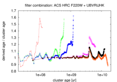
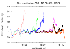
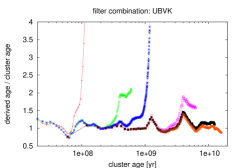
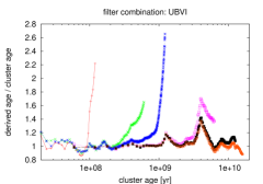
Figure 9: Derived ages of dissolving star clusters with t_95% in the range 100 Myr – 60 Gyr (from left to right: 100, 500 Myr, 1, 5, 10, 20 Gyr), using standard models, for a number of filter combinations. Upper left panel: ACS HRC F220W + standard UBVRIJHK, top right: ACS HRC F220W + standard UBVK, bottom left: standard UBVK, bottom right: standard UBVI. Shown is the ratio between the age derived using standard models and the age the dissolving cluster has.

4 Validation of the models

In this section we will investigate several uncertainties inherent to our models, as well as comparing our new models with models previously released by our group.

All the following values are maximum differences from the standard models of a given parameter in a given time interval, unless otherwise noted. In many cases the maximum deviations occur in the final stages of cluster dissolution, and for the longest total disruption times $<$ maximum model age. If we would have chosen a maximum model age of 13 Gyr instead of 16 Gyr, the maximum deviations would generally be slightly smaller.

For the different issues discussed in this section, we also publish a few test cases on our webpage, illustrating the impact of different initial-final mass relations, isochrones and parametrisations of the mass function evolution on colours and masses/ mass-to-light ratios. For the parametrisations of the mass function evolution we select a few disruption times for presentation on the webpage, while for the initial-final mass relations and isochrones we present only data without disruption (i.e. pure stellar evolution) to avoid confusion.

4.1 Parametrisation of mass function slope evolution

As discussed earlier, the mass function slope evolution is derived from a subset of N-body simulations by BM03. The subset was selected to cover the parameter space well, while limiting the impact of low-number statistics (see Sect. 2.3).

The fit to the data of the time evolution of the mass function slopes has formally a very high accuracy due to the large number of data points. However, as shown in Figs. 3 and 3, the N-body models show an intrinsic spread around the fitted function. We quantified this spread to have a median value $\leq$ $\pm$15% for ages $\geq$ 1/3 t_95%. For younger ages, this relative spread is larger, however the median of the absolute spread is small, $\leq$ $\pm$0.02-0.03 change in the slope.

We test the impact of this spread by calculating models for which the time-dependent part of the mass function slope is reduced/increased by 15%. We find, as expected, the change in the “high-mass slope” (i.e. for masses $\geq$ 0.3 M_⊙) to be of primary importance, while the time-dependent contribution from stars with masses $\leq$ 0.3 M_⊙ changes the photometry only mildly.

As the mass evolutions of the cluster (total, luminous and remnant mass) were derived independent of the mass function evolution, the masses are not affected.

The impact of this uncertainty on the colors is small: the changes induced for the models with the shortest disruption time t_95% (i.e. 100 Myr) and the colors with the longest wavelength coverage (i.e. V-K) reach $\approx$ 0.07mag at final disruption. These changes decrease rapidly with increasing disruption time and decreasing wavelength coverage.

For ages ${\rm t\leq t_{95\%}}$ the magnitudes change by $\sim$ 0.15 – 0.2 mag (with the changes slightly larger for the shortest t_95% and red passbands). As the mass is unaltered, this directly translates into a change in the M/L ratio by 15 – 20%.

For ages ${\rm t>t_{95\%}}$ both magnitudes and M/L ratios diverge from the models using the best fitting relation for the time evolution of the mass function slopes. Models with a weaker time evolution are increasingly brighter and have consequently lower M/L ratios.

In Fig. 10 we illustrate the effects of enhancing the MF evolution by 15%. Diminishing the effects of MF evolution by 15% gives quantitatively similar results with the changes w.r.t. the standard models going in the opposite direction. The V-K colour evolutions are the most extreme cases: Effects become smaller for shorter wavelength coverage and longer disruption times.

Figure 10: Integrated V-K colour (left panel) and M/L_V ratio (right panel) for a Kroupa IMF, solar metallicity, our standard isochrones, a range of cluster disruption times, with the effect of MF evolution enhanced by 15% w.r.t.the standard models. Shown are the quantities relative to the respective quantities of our standard models. Diminishing the effect of MF evolution by 15% yields quantitatively similar results, however, the changes are in the opposite direction.

In summary, the uncertainty induced by the spread of N-body model data around the fitted time evolution of the mass function slopes has an impact on the model predictions. However, for ages ${\rm t\leq t_{95\%}}$ the induced uncertainties are much smaller than the error one makes by not taking into account the effect of preferential mass loss and cluster dissolution. In addition, we aim at describing the average cluster.

4.2 Initial-final mass relations

Our model results, especially the M/L ratios discussed in Sect. 3.2, depend on the treatment of stellar remnants. The remnants mass is calculated from the progenitor star’s initial mass and the adopted initial-final mass relation (IFMR), which accounts for mass loss during the life of the progenitor star and due to the “death” of the star and the formation of the remnant.

The IFMR for white dwarfs used in this work is based on the work by Weidemann & Koester (1983) (hereafter “Weidemann83”). As the IFMR is still uncertain, we tested our choice by adopting different IFMRs for white dwarfs, namely by Weidemann (2000) (hereafter “Weidemann00”), by Kalirai et al. (2008) (hereafter “Kalirai08”) and the prescription by Hurley et al. (2000) (hereafter “HPT00”). For the latter one we also adopt their IFMR for neutron stars, while for all other IFMRs we adopt Nomoto & Hashimoto 1988.

Changes discussed below are w.r.t. our standard IFMR Weidemann83.

We find the IFMR to be of minor influence on the results for ages ${\rm t\leq t_{95\%}}$: the total mass changes by maximum 2 – 3%, while the luminous mass changes by 4% and 6% (for Weidemann00/Kalirai08 and HPT00, respectively). This translates into magnitude changes of $\sim$0.05mag and $\sim$0.07 mag (for Weidemann00/Kalirai08 and HPT00, respectively). The associated effect on the M/L ratios is $\sim$4.5% and $\sim$6.5% (for Weidemann00/Kalirai08 and HPT00, respectively).

For larger ages ${\rm t\geq t_{95\%}}$ the results eventually diverge. However, only in the last 5% of a cluster’s lifetime the total mass differs by more than 10%, regardless of the choice of IFMR.

In Fig. 11 we show the impact of the chosen IFMR on the M/L_V ratio for infinite disruption time.

Figure 11: M/L_V ratio for a Kroupa IMF, solar metallicity, no cluster dissolution and the 3 alternative IFMRs discussed in the text. Shown are the quantities relative to the respective quantities of our standard models.

4.3 Isochrones

Our choice of isochrones (i.e. isochrones from the Pavoda group, first presented in Bertelli et al. 1994 with later updates of the Padova group concerning the TP-AGB phase = “updated Padova94”) is driven by the following points:

1. For consistency with galev models of galaxies we require isochrones which cover the full mass range up to high masses (ideally up to $\sim$ 120 M_⊙) to properly model ongoing star formation in galaxies.

2. Likewise models covering a wide range in metallicities is desired to consistently model old/metal-poor globular clusters and young/metal-rich star clusters formed in nearby starbursts, as well as to model galaxies consistently from the onset of star formation to their present stage.

3. The models should cover all relevant evolutionary stages of these stars, especially the very luminous phases (for our study especially the TP-AGB phase is of prime importance, but also early stages like supergiants are important).

We regret that recent high-quality isochrone calculations (e.g. Girardi et al. 2000; Yi et al. 2001; Cariulo et al. 2004; Pietrinferni et al. 2004, 2006; Bertelli et al. 2008) are all focussing on “low-mass” stars (maximum up to $\sim$ 10 M_⊙, though Bertelli et al. 2008 announce models up to 20 M_⊙ for the near future) and/or do not fulfil one or more criteria mentioned above. However, stars more massive than $\approx$ 10 M_⊙ contribute significantly to the chemical enrichment and the light of young star clusters and most galaxies.

The only models fulfilling all mentioned criteria are models by the Padova group (Bertelli et al. 1994 plus TP-AGB updates) and by the Geneva group (Schaller et al. 1992; Charbonnel et al. 1993; Schaerer et al. 1993).

As the main focus in this paper is on systems older than $\sim$ 100 Myr we prefer the updated Padova94 isochrones over the Geneva isochrones.

The alternative solution, to combine isochrones from different groups/epochs, was rejected as consistency cannot be ensured.

We tested solar-metallicity isochrones by Cariulo et al. (2004); Pietrinferni et al. (2004); Marigo et al. (2008) (also known as “Pisa/GIPSY”, “BASTI” and “new Padova”, respectively) with respect to the updated Padova94 isochrones we used in this study, and derived star cluster models for test purposes. While the Pisa isochrones are offset from all other isochrones (they are generally significantly hotter, but are based on more limiting input physics), the other isochrones are in overall good agreement with the updated Padova94 isochrones. Small differences include:

• For increasing age, the BASTI main-sequence turn-off temperature goes from slightly cooler than the updated Padova94 to slightly hotter (by a few per cent). This results in an increasing deviation of U-/B-band magnitudes compared to the updated Padova94 isochrones by up to 0.5mag. The new Padova isochrones show much smaller deviations $\la$ 0.15mag in these passbands. Contrary, for both BASTI and new Padova, colours like U-B or B-V deviate for most of the time by $\la$ 0.1mag, and for the majority of time by $\la$ 0.05mag from the updated Padova94 models.

• Overall, the RGBs and AGBs in the BASTI and new Padova isochrones are hotter than in the updated Padova94 isochrones. Especially stars with the highest luminosities on the RGB/AGB are treated differently. For ages younger than $\sim$1 Gyr, the test models deviate significantly, both from our standard model as well as from each other. For ages $\ga$2 Gyr, the BASTI and new Padova isochrones give comparable optical/NIR colours V-I and V-K, but are offset from the updated Padova94 models by $\sim$ -0.1mag (V-I) and $\sim$ -0.6mag (V-K), in the sense that the updated Padova94 models are redder.

• The BASTI “non-canonical models” (i.e. with core convective overshooting during the H-burning phase) are closer to the updated Padova94 isochrones than their “canonical models” (i.e. without overshooting).

• The mass lost due to stellar evolution differs by 2% (new Padova) – 7% (BASTI) when compared to the updated Padova94 isochrones.

• The relative effects induced by the preferential mass loss (i.e. the difference between models with and without the effects of cluster dissolution) are qualitatively robust against the choice of isochrones. Small quantitative differences are present. However, they tend to be even stronger for the new isochrones than for the updated Padova94 isochrones.

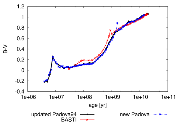
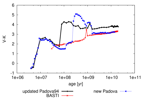
Figure 12: Integrated B-V (left panel) and V-K colour (right panel) for a Kroupa IMF, solar metallicity, no cluster dissolution and 3 different sets of isochrones: the “upgraded Padova94” (our standard models, black lines), the “BASTI” isochrones (red lines, Pietrinferni et al. 2004) and the “new Padova” isochrones (blue dotted lines, Marigo et al. 2008).

For two example colours (B-V and V-K), the time evolution for a standard SSP (i.e. without cluster dissolution) at solar metallicity is shown in Fig. 12. The blue colour B-V, dominated by hot stars mainly on the main sequence, shows good agreement between the investigated isochrones. The V-K colour for ages younger than $\approx$1.5 Gyr is in strong disagreement between all three isochrones, up to 2.8mag difference around an age of 300 Myr, showing strong differences in the treatment of the AGB phase. For older ages, the new Padova agrees well with the BASTI isochrones, but both are offset from the upgraded Padova94 by $\approx$0.6mag.

To account for the uncertainty in the choice of isochrones, we will build grids of dissolving cluster models, based on the BASTI, the new Padova and the Bertelli et al. (2008) (once the extension to higher masses is published) isochrones, respectively, and release it on our webpage. These models will also employ the Kalirai et al. (2008) initial-final mass relation.

4.4 Comparison with earlier work

The new models presented here supersede our earlier work (Lamers et al. 2006). In Lamers et al. (2006) we approximated the changes in the mass function by a time-dependent lower mass limit (i.e. assuming that only the lowest-mass stars are removed from the cluster, while higher-mass stars might only be removed by stellar evolution) and scaled our models to match the total mass in stars with M $<$ 2 M_⊙ with the BM03 simulations. Recently, this approach has been improved by Kruijssen & Lamers (2008) by incorporating the effects of stellar remnants for clusters of different initial masses and different total disruption times for a range of metallicities. In that paper, the consequences of various physical effects on the photometry and M/L ratios have been investigated, e.g. initial mass segregation, the role of white dwarfs and neutron stars, the role of metallicity etc..

Due to the normalisation procedure, the total masses of the earlier models differs negligibly from the new models. However, the number of bright stars in the new models decreases slower than in the old models by Lamers et al. (2006) (the models by Kruijssen & Lamers 2008 represent already an improvement over the earlier work, and are more consistent with the work presented here). Hence the new models are brighter than the old models, especially for short disruption times. Consequently, the new mass-to-light ratio is lower, by 20 – 40%.

The new models are redder than the older ones, because the changing slope of the mass function slowly depopulates the (blue) main-sequence turn-off region already early on. Contrary, in the older models stars in the main-sequence turn-off region are removed more abruptly when the lower mass limit reaches the turn-off mass.

Before the lower mass limit reaches the turn-off mass in the old models, colors get slightly bluer for a short time, because almost all main sequence stars redder than the turn-off have been removed by then. This feature is not present in the new models, due to the more gradual mass loss. In addition, the old models show a strong reddening in their final stages, as the star cluster contains exclusively red giants/AGB stars (plus stellar remnants). Also this feature is not strongly present in the new models, as the mass function even close to total disruption covers a wider range.

5 Conclusions

We presented a novel suite of evolutionary synthesis models, which accounts for the dynamical evolution of star clusters in a tidal field in a realistic manner. The dynamically induced changes in the stellar MF within the cluster and the overall mass loss of stars from the cluster into the surrounding field population is consistently taken into account. The models are made publicly available on our webpages http://www.phys.uu.nl/$\sim$anders/data/SSP_varMF/ and http://data.galev.org for general use.

Based on the simulations presented in BM03, we improved the parametrisation of the time evolution of the MF slope changes. We then combined this new description of the MF slopes with our galev evolutionary synthesis models. The resulting models, calculated for a range in metallicities and total cluster disruption times, were shown to deviate significantly from the canonical evolutionary synthesis models which neglect the effects of dynamical cluster evolution. Depending on the total cluster disruption time and the colour index under investigation, differences up to 0.7mag (and in a large number of cases exceeding 0.1mag) were found. These deviation were shown to lead to significant misinterpretations of observation. E.g. cluster age determinations can be wrong by 20 – 50%, in extreme cases by up to a factor $\sim$2 – 3. These deviations were found to depend strongly on the filter combination used to derive the ages: combinations including near-IR filters tend to be more sensitive to the changing MF, while for large wavelength coverage and/or large numbers of filters the deviations are still significant but generally smaller.

Also the M/L ratios are strongly affected, and therefore photometric cluster masses derived from observations. For the largest part of a cluster’s lifetime the M/L ratios are significantly below the canonical values (by up to a factor $\sim$3 – 7). In late stages of cluster dissolution the M/L ratios exceed the standard values, as the cluster mass gets increasingly dominated by stellar remnants. This period can last for up to $\sim$16% of the cluster’s total disruption time. In both cases, the M/L ratios are strongly time-dependent. For fixed cluster age and/or fixed local disruption time, the dependence of M/L ratios on the presently observed cluster mass was investigated. They are broadly consistent with observations, although the observations show large scatter and uncertainties.

Our results confirm the trends in the evolution of colour and mass-to-light ratios of dissolving clusters, obtained by Kruijssen & Lamers (2008) and Kruijssen (2008), who used a simplified description of the changes in the mass function due to the preferential loss of low-mass stars in star clusters.

While the absolute values of our results depend on our choice of input physics, the general behaviour is robust against these choices. We will update our models whenever better input physics becomes available.

6 Acknowledgements

PA acknowledges funding by NWO (grant 614.000.529) and the European Union (Marie Curie EIF grant MEIF-CT-2006-041108). PA and HL would like to thank the ISSI in Bern/Switzerland for their hospitality and support. PA would like to acknowledge fruitful discussions with Ines Brott and Rob Izzard, as well as with Diederik Kruijssen. Many thanks to Marina Rejkuba for a critical reading of the paper and asking the right questions. In addition, thanks to Marina Rejkuba and Steffen Mieske for kindly providing part of the observational data. PA is in Uta Fritzes debt for many years of teaching, advice and fruitful collaboration. This research was supported in part by the National Science Foundation under Grant No. PHY05-51164.

References

- Anders et al. (2004a) Anders, P., Bissantz, N., Fritze-v. Alvensleben, U., & de Grijs, R. 2004a, MNRAS, 347, 196
- Anders et al. (2004b) Anders, P., de Grijs, R., Fritze-v. Alvensleben, U., & Bissantz, N. 2004b, MNRAS, 347, 17
- Anders & Fritze-v. Alvensleben (2003) Anders, P. & Fritze-v. Alvensleben, U. 2003, A&A, 401, 1063
- Bastian & Goodwin (2006) Bastian, N. & Goodwin, S. P. 2006, MNRAS, 369, L9
- Baumgardt et al. (2008) Baumgardt, H., De Marchi, G., & Kroupa, P. 2008, ApJ, 685, 247
- Baumgardt & Makino (2003) Baumgardt, H. & Makino, J. 2003, MNRAS, 340, 227
- Baumgardt & Mieske (2008) Baumgardt, H. & Mieske, S. 2008, MNRAS, 1255
- Bertelli et al. (1994) Bertelli, G., Bressan, A., Chiosi, C., Fagotto, F., & Nasi, E. 1994, A&AS, 106, 275
- Bertelli et al. (2008) Bertelli, G., Girardi, L., Marigo, P., & Nasi, E. 2008, A&A, 484, 815
- Bicker et al. (2002) Bicker, J., Fritze-v. Alvensleben, U., & Fricke, K. J. 2002, A&A, 387, 412
- Bicker et al. (2004) Bicker, J., Fritze-v. Alvensleben, U., Möller, C. S., & Fricke, K. J. 2004, A&A, 413, 37
- Boutloukos & Lamers (2003) Boutloukos, S. G. & Lamers, H. J. G. L. M. 2003, MNRAS, 338, 717
- Bruzual & Charlot (2003) Bruzual, G. & Charlot, S. 2003, MNRAS, 344, 1000
- Cariulo et al. (2004) Cariulo, P., Degl’Innocenti, S., & Castellani, V. 2004, A&A, 421, 1121
- Cerviño & Luridiana (2004) Cerviño, M. & Luridiana, V. 2004, A&A, 413, 145
- Cerviño & Luridiana (2006) Cerviño, M. & Luridiana, V. 2006, A&A, 451, 475
- Cerviño & Mollá (2002) Cerviño, M. & Mollá, M. 2002, A&A, 394, 525
- Charbonnel et al. (1993) Charbonnel, C., Meynet, G., Maeder, A., Schaller, G., & Schaerer, D. 1993, A&AS, 101, 415
- Chen et al. (2007) Chen, L., de Grijs, R., & Zhao, J. L. 2007, AJ, 134, 1368
- Dabringhausen et al. (2008) Dabringhausen, J., Hilker, M., & Kroupa, P. 2008, MNRAS, 386, 864
- de Grijs & Anders (2006) de Grijs, R. & Anders, P. 2006, MNRAS, 366, 295
- de Grijs et al. (2004) de Grijs, R., Smith, L. J., Bunker, A., et al. 2004, MNRAS, 352, 263
- Fagiolini et al. (2007) Fagiolini, M., Raimondo, G., & Degl’Innocenti, S. 2007, A&A, 462, 107
- Fioc & Rocca-Volmerange (1997) Fioc, M. & Rocca-Volmerange, B. 1997, A&A, 326, 950
- Gieles et al. (2007) Gieles, M., Athanassoula, E., & Portegies Zwart, S. F. 2007, MNRAS, 376, 809
- Gieles et al. (2005) Gieles, M., Bastian, N., Lamers, H. J. G. L. M., & Mout, J. N. 2005, A&A, 441, 949
- Gieles & Baumgardt (2008) Gieles, M. & Baumgardt, H. 2008, MNRAS, 389, L28
- Gieles et al. (2006) Gieles, M., Portegies Zwart, S. F., Baumgardt, H., et al. 2006, MNRAS, 371, 793
- Giersz & Heggie (1997) Giersz, M. & Heggie, D. C. 1997, MNRAS, 286, 709
- Gill et al. (2008) Gill, M., Trenti, M., Miller, M. C., et al. 2008, ApJ, 686, 303
- Girardi et al. (2000) Girardi, L., Bressan, A., Bertelli, G., & Chiosi, C. 2000, A&AS, 141, 371
- Goodwin & Bastian (2006) Goodwin, S. P. & Bastian, N. 2006, MNRAS, 373, 752
- Gouliermis et al. (2004) Gouliermis, D., Keller, S. C., Kontizas, M., Kontizas, E., & Bellas-Velidis, I. 2004, A&A, 416, 137
- Harris (1996) Harris, W. E. 1996, AJ, 112, 1487
- Henon (1969) Henon, M. 1969, A&A, 2, 151
- Hurley et al. (2000) Hurley, J. R., Pols, O. R., & Tout, C. A. 2000, MNRAS, 315, 543
- Hurley et al. (2004) Hurley, J. R., Tout, C. A., Aarseth, S. J., & Pols, O. R. 2004, MNRAS, 355, 1207
- Kalirai et al. (2008) Kalirai, J. S., Hansen, B. M. S., Kelson, D. D., et al. 2008, ApJ, 676, 594
- Kassin et al. (2003) Kassin, S. A., Frogel, J. A., Pogge, R. W., Tiede, G. P., & Sellgren, K. 2003, AJ, 126, 1276
- Kroupa (2001) Kroupa, P. 2001, MNRAS, 322, 231
- Kruijssen (2008) Kruijssen, J. M. D. 2008, A&A, 486, L21
- Kruijssen & Lamers (2008) Kruijssen, J. M. D. & Lamers, H. J. G. L. M. 2008, A&A, 490, 151
- Kundu et al. (2005) Kundu, A., Zepf, S. E., Hempel, M., et al. 2005, ApJ, 634, L41
- Küpper et al. (2008) Küpper, A. H. W., Kroupa, P., & Baumgardt, H. 2008, MNRAS, 389, 889
- Lada & Lada (2003) Lada, C. J. & Lada, E. A. 2003, ARA&A, 41, 57
- Lamers et al. (2006) Lamers, H. J. G. L. M., Anders, P., & de Grijs, R. 2006, A&A, 452, 131
- Lamers et al. (2005a) Lamers, H. J. G. L. M., Gieles, M., Bastian, N., et al. 2005a, A&A, 441, 117
- Lamers et al. (2005b) Lamers, H. J. G. L. M., Gieles, M., & Portegies Zwart, S. F. 2005b, A&A, 429, 173
- Larsen et al. (2004) Larsen, S. S., Brodie, J. P., & Hunter, D. A. 2004, AJ, 128, 2295
- Larsen & Richtler (2004) Larsen, S. S. & Richtler, T. 2004, A&A, 427, 495
- Leitherer et al. (1999) Leitherer, C., Schaerer, D., Goldader, J. D., et al. 1999, ApJS, 123, 3
- Lejeune et al. (1997) Lejeune, T., Cuisinier, F., & Buser, R. 1997, A&AS, 125, 229
- Lejeune et al. (1998) Lejeune, T., Cuisinier, F., & Buser, R. 1998, A&AS, 130, 65
- Maccarone & Servillat (2008) Maccarone, T. J. & Servillat, M. 2008, MNRAS, 389, 379
- Maraston (2005) Maraston, C. 2005, MNRAS, 362, 799
- Marigo et al. (2008) Marigo, P., Girardi, L., Bressan, A., et al. 2008, A&A, 482, 883
- Marks et al. (2008) Marks, M., Kroupa, P., & Baumgardt, H. 2008, MNRAS, 386, 2047
- McLaughlin & van der Marel (2005) McLaughlin, D. E. & van der Marel, R. P. 2005, ApJS, 161, 304
- Mieske et al. (2008) Mieske, S., Hilker, M., Jordán, A., et al. 2008, A&A, 487, 921
- Mieske & Kroupa (2008) Mieske, S. & Kroupa, P. 2008, ApJ, 677, 276
- Nomoto & Hashimoto (1988) Nomoto, K. & Hashimoto, M. 1988, Phys. Rep, 163, 13
- Odenkirchen et al. (2003) Odenkirchen, M., Grebel, E. K., Dehnen, W., et al. 2003, AJ, 126, 2385
- Pietrinferni et al. (2004) Pietrinferni, A., Cassisi, S., Salaris, M., & Castelli, F. 2004, ApJ, 612, 168
- Pietrinferni et al. (2006) Pietrinferni, A., Cassisi, S., Salaris, M., & Castelli, F. 2006, ApJ, 642, 797
- Pryor & Meylan (1993) Pryor, C. & Meylan, G. 1993, in Astronomical Society of the Pacific Conference Series, Vol. 50, Structure and Dynamics of Globular Clusters, ed. S. G. Djorgovski & G. Meylan, 357–+
- Rejkuba et al. (2007) Rejkuba, M., Dubath, P., Minniti, D., & Meylan, G. 2007, A&A, 469, 147
- Salpeter (1955) Salpeter, E. E. 1955, ApJ, 121, 161
- Schaerer et al. (1993) Schaerer, D., Meynet, G., Maeder, A., & Schaller, G. 1993, A&AS, 98, 523
- Schaller et al. (1992) Schaller, G., Schaerer, D., Meynet, G., & Maeder, A. 1992, A&AS, 96, 269
- Schulz et al. (2002) Schulz, J., Fritze-v. Alvensleben, U., Möller, C. S., & Fricke, K. J. 2002, A&A, 392, 1
- Smith et al. (2007) Smith, L. J., Bastian, N., Konstantopoulos, I. S., et al. 2007, ApJ, 667, L145
- Spitzer & Shull (1975) Spitzer, Jr., L. & Shull, J. M. 1975, ApJ, 201, 773
- Tinsley (1968) Tinsley, B. M. 1968, ApJ, 151, 547
- Tinsley (1980) Tinsley, B. M. 1980, Fundamentals of Cosmic Physics, 5, 287
- Tinsley & Gunn (1976) Tinsley, B. M. & Gunn, J. E. 1976, ApJ, 203, 52
- Weidemann (2000) Weidemann, V. 2000, A&A, 363, 647
- Weidemann & Koester (1983) Weidemann, V. & Koester, D. 1983, A&A, 121, 77
- Worthey (1994) Worthey, G. 1994, ApJS, 95, 107
- Yi et al. (2001) Yi, S., Demarque, P., Kim, Y.-C., et al. 2001, ApJS, 136, 417