Dynamical Quantum Error Correction of Unitary Operations with Bounded Controls

Abstract

Dynamically corrected gates were recently introduced [Khodjasteh and Viola, Phys. Rev. Lett. 102, 080501 (2009)] as a tool to achieve decoherence-protected quantum gates based on open-loop Hamiltonian engineering. Here, we further expand the framework of dynamical quantum error correction, with emphasis on elucidating under what conditions decoherence suppression can be ensured while performing a generic target quantum gate, using only available bounded-strength control resources. Explicit constructions for physically relevant error models are detailed, including arbitrary linear decoherence and pure dephasing on qubits. The effectiveness of dynamically corrected gates in an illustrative non-Markovian spin-bath setting is investigated numerically, confirming the expected fidelity performance in a wide parameter range. Robutness against a class of systematic control errors is automatically incorporated in the perturbative error regime.

I Introduction

The technological advances promised by quantum information processing (QIP) science require an unprecedented level of control in characterizing, manipulating, and measuring quantum systems DiVincenzo (2000). In reality, no quantum system may be perfectly isolated from its surrounding environment and available means for control and measurement are unavoidably limited. As a results, deviations from the intended dynamical evolution arise, which are collectively referred to as ‘errors’. Active quantum error correction (QEC) methods aim to detect and counteract the effects of errors during both quantum storage and processing of information via non-trivial quantum gates Nielsen and Chuang (2000). Given limited control resources, accurate quantum computation (QC) on an arbitrarily large (scalable) QI processor is only possible if QEC is implemented fault-tolerantly, that is, more errors is removed than is generated when operations are themselves imperfect. The theory of fault-tolerant QEC (FTQEC) guarantees that this is possible in principle, provided that the error per gate (EPG) is below a minimum threshold Kitaev (1997); Preskill (1998); Knill et al. (1998). Unfortunately, while architectures which can tolerate EPGs comparable with experimentally achieved values have been proposed Steane (2003); Knill (2005), the corresponding resource overheads remain prohibitive for existing QIP test-beds. Thus, QEC strategies which can effectively reduce errors at the physical level are both crucial for boosting control fidelities in current quantum devices and, in the long run, for enabling fault-tolerant QC.

While traditional QEC methods achieve information protection by resorting to suitable redundant encodings and non-unitary quantum operations, dynamical quantum error correction (DQEC) aims to counteract the effects of decoherence in a quantum system in a purely ‘open-loop’ fashion, that is, solely based on suitable unitary (Hamiltonian) control. Historically, dynamical procedures for effectively removing unwanted couplings and/or evolution by time-dependent ‘coherent averaging’ have decades of tradition in nuclear magnetic resonance (NMR) spectroscopy Haeberlen (1976), resulting in an unmatched degree of coherent control in liquid-state nuclear-spin qubits Cor ; Ryan et al. . In particular, dynamical decoupling (DD) sequences in NMR are early examples of DQEC for a closed quantum system, specifically designed to ‘time-suspend’ the underlying spin evolution by achieving a net trivial (identity) propagator, or noop gate. In the QIP context, DD methods have evolved into a powerful and versatile framework for achieving decoherence suppression in non-Markovian open quantum systems in a variety of control settings Viola and Lloyd (1998); Viola et al. (1999a). While recent theoretical developments include the exploitation of randomized design Viola and Knill (2005); Santos and Viola (2006), and the construction of concatenated CDD and optimal UDD DD sequences, the growing practical significance of DQEC methods is witnessed by the intense parallel effort in the experimental QIP community. Following simple proof-of-principle demonstrations in a single-photon polarization interferometer Berglund , DD in its simplest (so-called ‘bang-bang’) form has been successfully implemented by now in solid-state nuclear quadrupole qubits Fraval et al. (2005), fullerene qubits Morton et al. (2006), coupled electron-nuclear systems Morton et al. (2008), flying polarization qubits Damodarakurup et al. , and, most recently, trapped ions Bie .

Although the advances mentioned above demonstrate the usefulness of DQEC toward removing unwanted decoherence in between control pulses and achieving a robust noop implementation, full-fledged DQEC demands that decoherence be removed both in between and during control pulses, while implementing a robust non-trivial (non-identity) quantum gate. Dynamically corrected gates (DCGs) were introduced in Ref. Khodjasteh and Viola, 2009a precisely to meet this goal. As opposed to readily available ‘primitive gates,’ which effect a unitary operation on the system with a ‘bare’ EPG, each DCG consists of a suitably designated sequence of control inputs in such a way that the desired target transformation is effected with a net reduced EPG. DCGs are inspired by both composite-pulse techniques for reducing classical control errors (in particular, so-called ‘fully compensating’ or ‘universal rotation’ sequences) Levitt (1986); Alway and Jones (2007); Brown et al. (2004); Khaneja et al. (2005); Hill (2007) as well as strongly-modulating pulses Fortunato et al. (2002); Boulant et al. (2003); Luy et al. (2005) for high-fidelity ‘soft’ pulses in NMR, while differing from either strategy in important ways. Specifically, DGCs compensate for error evolution due to a dynamical quantum environment over which neither quantitative knowledge nor direct control is assumed. Although DCG constructions are useful only in the short gating time/weak coupling limit and cannot counter stochastic control errors, a key advantage is that no extra qubits or measurement capabilities are needed, thanks to the underlying open-loop control design. On the one hand, DCGs relate to ongoing effort on improving pulse-shaping methods in order to better accommodate physical constraints and/or increase robustness against different errors. In particular, DD-inspired constructions for pulses capable to ‘self-refocus’ unwanted couplings have been recently investigated in Pasini et al. (2008); Pryadko and Quiroz (2008); Sengupta and Pryadko (2005). These efforts nonetheless consider a specific control task (noop implementation) and/or do not incorporate the effect of generic quantum errors. DCGs, on the other hand, are applicable to any desired unitary operation, and have the flexibility to handle a generic class of non-Markovian error models on qubits. Furthermore, DCGs are designed having high portability in mind, so that they can replace the already available gates whenever appropriate (mild) compatibility conditions are met. Substituting primitive gates with DCGs can then significantly lower physical EPGs, ultimately paving the way for more practical FTQEC architectures.

In this paper, we expand our analysis of DCG constructions with the twofold goal of describing in detail the mathematical groundwork underlying the results of Khodjasteh and Viola (2009a), as well as further demonstrating the flexibility and potential of DCGs for high-fidelity quantum control in open quantum systems. The content is organized as follows. In Sec. II, we formulate the DCG synthesis problem in a control-theoretic setting, and describe the mathematical assumptions and concepts that are relevant to the subsequent steps. In Sec. III, we review the fundamentals of DD methods based on realistic bounded-strength controls, within so-called Eulerian DD Viola and Knill (2003). In particular, we re-interpret the latter as a special DCG aimed at quantum state preservation, and prove a ‘No-Go’ theorem that restricts the portability of ‘black-box’ DCGs beyond the noop gate. Sec. IV shows how to evade the No-Go theorem and describes general DCG constructions in detail. Special attention is paid to elucidating the compatibility requirements that emerge for physically relevant qubit error models, including arbitrary linear decoherence and pure dephasing. In Sec. V, a concrete spin-bath decoherence scenario is used as a case study to numerically validate DCGs and to gain insight into open-system and control features which affect their performance. In Sec. VI, we elaborate on the effects of additional error evolution induced by control non-idealities and/or internal unitary drifts. A summary of the main findings and open questions conclude in Sec. VII.

II Control-theoretic setting for dynamical error correction

Consider an isolated quantum system $S$ with an internal Hamiltonian $H_{S}$ which can be controlled through the application of a time-dependent Hamiltonian $H_{\text{ctrl}}(t)$. This control enables us to perform certain quantum tasks on $S$. For example, by turning off $H_{S}$ completely, an arbitrary state of $S$ may be preserved. Complex control tasks such as unitary quantum gates and algorithms composed of such gates may also be performed by modulating $H_{S}$ through $H_{\text{ctrl}}(t)$. In reality, however, $S$ interacts with an environment system (referred to as the ‘bath’ $B$ henceforth) via an interaction Hamiltonian $H_{SB}$. In the presence of $H_{SB}$, a designated control sequence on $S$ is not sufficient to accurately implement a desired evolution, due to non-unitary decoherence errors that are induced once the bath degrees of freedom are traced out.

Let, as usual, the initial joint state of $S$ and $B$ be separable, with $\rho^{\text{in}}=\rho_{S}^{\text{in}}\otimes\rho_{B}^{\text{in}}$, and $\rho_{S}^{\text{in}}=|\psi_{\text{in}}\rangle\langle\psi_{\text{in}}|$. Ideally, the action of a target unitary gate $Q$ effected over a gating interval $[0,T]$ should result in a final state of the form $\rho_{SB}^{\text{fin}}(T)=Q^{\dagger}\rho_{S}^{\text{in}}Q\otimes\rho_{B}^{\text{fin}}(T)$, for some (irrelevant) final state $\rho_{B}^{\text{fin}}(T)$ of the bath. In contrast, the actual action of the gate in the presence of $H_{SB}$ results in the combined joint state $\rho_{SB}^{\text{err}}(T)$, and the system ends up in an erroneous reduced state $\rho_{S}^{e}(T)=\text{Tr}_{B}(\rho_{S}^{\text{err}}(T))\neq Q^{\dagger}\rho_{S}^{\text{in}}Q$. While different measures may be envisioned to quantify the deviation between the intended and the actual evolution, the resulting EPG will be proportional to the gating time $T$, as well as to the overall ‘error strength,’ appropriately defined. In essence, DCG constructions aim to improve the scaling of physical EPGs with the gating time in the limit where the latter is sufficiently small, so that a perturbative approach is meaningful. That is, a gate $Q_{\text{DCG}}$ is an $\ell$-th order DCG if it obeys

$$\frac{\text{EPG}^{[\ell]}}{\text{EPG}^{[0]}}=O(T^{\ell}),\;\;\;\ell\geq 1,$$ (1)

where the asymptotic $O$-notation is used to signify the limit where the zero-th order bare EPG is close to 0. If desired, the above defining condition for a DCG may be expressed in terms of gate fidelity improvement once a specific fidelity metric is chosen and is related to the EPG amplitude in Eq. (1). Let, for instance, $f_{Q}$ denote the worst-case fidelity in implementing $Q$ Nielsen and Chuang (2000),

$$f_{Q}=\min_{|\psi_{\text{in}}\rangle}\,\text{Tr}\sqrt{\sqrt{\rho_{S}^{\text{err}}}\,{\rho_{S}^{\text{fin}}}\,\sqrt{\rho_{S}^{\text{err}}}}.$$ (2)

By taking the ‘infidelity’ $(1-f_{Q})$ as a measure of the gate error probability, a $\ell$-th order DCG implies an improvement ratio on the order of Brown et al. (2004); Terhal and Burkard (2005); Viola and Knill (2005)

$$r^{[\ell]}=\frac{1-f_{Q}\;\>}{1-f_{Q_{\text{DCG}}}^{[\ell]}}=O(T^{-2\ell}),$$ (3)

where $f_{Q_{\text{DCG}}}$ is the fidelity of implementation of a sequence of primitive gates whose fidelities are all similar and given by $f_{Q}$.

In this paper we will only focus on first-order DCGs ($\ell=1$), by postponing the construction and characterization of higher-order DCGs to a separate forthcoming analysis Khodjasteh and Viola (2009b).

II.1 Error model assumptions

Let $S$ consist of $n$ qubits, and let $B$ represent another quantum system over which knowledge is limited and no direct control is available. The free evolution of $S$ and $B$ in the combined Hilbert space $\mathcal{H}=\mathcal{H}_{S}\otimes\mathcal{H}_{B}$ is described by a bare internal Hamiltonian $H_{\text{int}}$ of the form

$$H_{\text{int}}=H_{S}\otimes I_{B}+H_{SB}+I_{S}\otimes H_{B},$$ (4)

where $I_{S}$ ($I_{B}$) is the identity operator in the operator space ${\cal B}(\mathcal{H}_{S})$ [${\cal B}(\mathcal{H}_{B}$)], respectively. Otherwise obvious tensor products components will be dropped from now on; e.g., $H_{B}$ will be understood as $I_{S}\otimes H_{B}$. The interaction Hamiltonian $H_{SB}$ is responsible for decoherence effects whereby initially separable states of $S$ and $B$ become entangled and loose their capacity for QIP. The typical time scale over which such effects become significant (loosely referred to as the ‘decoherence time’) depends in general on both $H_{SB}$ and various features of the bath, including $\rho_{B}^{\text{in}}$ Zurek (2003); Breuer and Petruccione (2002). Without loss of generality, $H_{SB}$ can be expanded as $H_{SB}=\sum_{\gamma}S_{\gamma}\otimes B_{\gamma}$, where $\{S_{\gamma}\}$ is an (Hermitian) operator basis for ${\cal B}(\mathcal{H}_{S})$, such as arbitrary products of Pauli operators on the $i$-th qubit, denoted by $\{S_{\alpha}^{(i)}\}$ ($\alpha\in\{I,X,Y,Z\}\equiv\{0,1,2,3\}$), and $B_{\gamma}$ being non-zero but otherwise unspecified bath operators. In most circumstances, the dominant terms in $H_{SB}$ belong to a restricted subspace of all possible coupling operators. In particular, the linear decoherence model is defined by letting:

$$H_{SB}^{\text{lin}}=\sum_{i=1}^{n}\sum_{\alpha=1}^{3}S_{\alpha}^{(i)}\otimes B_{\alpha}^{(i)}.$$ (5)

Physically, the class of error models described by Eq. (5) allows for arbitrary combinations of phase- and amplitude- damping processes involving a generic axis and degree of correlations between different qubits (from independent to fully collective linear interactions) Knill et al. (2000). In DQEC approaches, it is useful to associate an error subspace $\Omega_{e}\subset{\cal B}({\cal H})$ to the set of error generators we wish to suppress. For linear decoherence,

$$\Omega_{e}=\text{span}\,\{S_{\alpha}^{(i)}\otimes B\,|\,\forall\alpha,i;\;B\in{\cal B}({\cal H}_{B})\}\equiv\Omega_{e}^{\{1\}}$$ (6)

includes arbitrary system-bath operators that induce single-qubit errors on $S$. Also notice that the strength of the system-bath interaction Hamiltonian is constrained to be sufficiently weak in order for both QEC and DQEC to be useful in practice. This motivates assuming that both ${H_{SB}}$ and ${H_{B}}$ are bounded in an appropriate norm, although otherwise potentially unknown. The unitarily invariant operator norm $\left\|\cdot\right\|$ Bhatia (1997) will be used throughout our analysis.

If $H_{SB}$ is not present, a desired unitary operation $Q$ on $S$ can be generated, as mentioned earlier, by adjoining a semi-classical controller, described by a time-dependent Hamiltonian $H_{\text{ctrl}}(t)$. Depending on the system and control specifications, certain components of the internal system Hamiltonian might be essential to ensure universal controllability, whereas other will induce unintended (unitary) error evolution. In general, we may thus decompose $H_{S}=H_{S,g}+H_{S,e}$, where the separation into the gating and error contribution depends on the target transformation $Q$; for instance, $H_{S}\equiv H_{S,e}$ for noop, $Q=I_{S}$. In the presence of $H_{SB}$, let the total error Hamiltonian be defined by

$$H_{e}=H_{S,e}+H_{SB}+H_{B},$$ (7)

and, correspondingly, we represent the control action in terms of a gating Hamiltonian of the form

$$H_{\text{gate}}(t)\equiv H_{\text{gate}}(t)\otimes I_{B}=H_{\text{ctrl}}(t)+H_{S,g}.$$ (8)

In principle, a perfect implementation of $Q$ could still be ensured through infinitely strong, instantaneous gating Hamiltonians, during which $H_{e}$ has no time to act. However, this ideal scenario cannot be achieved in reality, although it may be realized approximately. Even if $H_{SB}\neq 0$, it may be useful to have a way for comparing operators in ${\cal B}(\mathcal{H})$ which differ only through directly uncontrollable pure-bath terms such as $H_{B}$. This can be accommodated by defining equivalence classes of operators: We say that $X$ is equal to $Y$ modulo the bath (mod$B$ for short) iff their difference is a pure-bath operator,

$$X=Y\text{ mod$B$}\Longleftrightarrow\ \exists X_{B}:\ X-Y=I_{S}\otimes X_{B},$$

where $X_{B}$ is an operator acting on $B$. For example, $H_{gate}(t)+H_{B}=H_{gate}(t)\text{ mod$B$}$. With this in mind, we use the words ideal or desired to refer to cases with $H_{e}=0$ mod$B$, where gates can be perfectly implemented by a suitable closed-system protocol $H_{\text{gate}}(t)$ over time $T$. Furthermore, we will primarily focus on open-system decoherence errors, that is, we will treat $H_{SB}$ as the leading source of errors in Eq. (7), by assuming that:

(a1) Perfect control assumption: No additional errors are introduced by the controller;

(a2) Driftless system assumption: No additional errors are introduced by the system’s internal evolution.

Assumption (a1) implies that the applied control Hamiltonian $H_{\text{ctrl}}(t)$ is perfect, subject to operational constraints to be specified later (Sec. II.2). While realistic controls will suffer in general of both systematic and stochastic (random) imperfections, these errors are intrinsically classical in nature. Likewise, assumption (a2) is partly justified by the fact that $H_{S}$ is fully known and, in the closed-system limit, complete control over $S$ is available. Once DCG constructions are found under the above simplifying assumptions, it is at least in principle conceivable that simultaneous compensation of classical and quantum (unitary and decoherence) errors could be achievable by suitably merging DCG constructions with existing robust control techniques, although several non-trivial aspects may remain. While additional discussion is deferred to Sec. VI), the impact of control imperfections will be also numerically assessed in Sec. V.

II.2 Control assumptions and error measure

Our goal is to use available control resources to generate unitary gates on $S$ while minimizing the sensitivity of the gate action to the error Hamiltonian $H_{e}$. In practice, allowed manipulations will be restricted by a number of constraints, which can be identified by writing

$$H_{\text{ctrl}}(t)=\sum_{u}h_{u}(t)V_{u}\equiv\sum_{u,\gamma}f_{\gamma}^{u}(t)S_{\gamma},$$ (9)

in terms of a subset of admissible control Hamiltonians $\{V_{u}\}$ and of control inputs $\{h_{u}(t)\}$, the latter being real-valued controllable functions of time. Limited ‘pulse-shaping’ capabilities may additionally restrict the values attainable by the control inputs $h_{u}(t)$ and/or their derivatives. Two main constraints will be incorporated into the present DCG design:

(c1) Finite power, which requires bounded control amplitudes, $h_{u}(t)\leq h_{\text{max}}$;

(c2) Finite bandwidth, which requires a bounded Fourier spectrum, hence a minimum time scale $\tau_{\text{min}}$ for modulation.

A ‘primitive gate’ will refer to a physically available gate used to generate more complex transformations. In the simplest case, a primitive gate may be implemented by turning on and off a single control Hamiltonian in the available set, subject to the above assumptions. A ‘control block’ will likewise refer to a time interval during which multiple primitive gates are applied sequentially in a predetermined manner. From the standpoint of universal QC, two different scenarios arise depending on whether the set of switchable control Hamiltonians $\{V_{u}\}$ in Eq. (9) supports a universal set of single- and two- qubit gates. If this is the case, $\{V_{u}\}$ generates a dense subset in SU$(2^{n})$, thus arbitrary unitary gates on $S$ may (ideally) be approximated to a desired accuracy by turning on and off primitive Hamiltonians in the set. Note that if no contribution from the internal Hamiltonian $H_{S}$ is needed to achieve universality ($H_{S,g}=0$), then to the purpose of DCG design we may effectively treat $H_{S}$ as a pure error ($H_{S}\equiv H_{S,e}$) and the problem as effectively driftless, in line with (a2).

Let $Q$ denote a quantum gate generated through the application of $H_{\text{ctrl}}(t)$ over the time interval $[0,T]$. Recalling Eq. (8), the gating propagator $U_{\text{gate}}(t,0)$, $t\in[0,T]$, can be defined in general as

$$U_{\text{gate}}(t,0) = T_{+}\Big{[}\exp\Big{(}-i\int_{0}^{t}H_{\text{gate}}(s)ds\Big{)}\Big{]},$$

such that $U_{\text{gate}}(T,0)=Q$. We use $U_{\text{gate}}(t)$ to denote $U_{\text{gate}}(t,0)$ when there is no ambiguity about the starting time of the gate. The overall propagator for the system plus bath is given by

$$U(T,0)=T_{+}\Big{[}\exp\Big{(}-i\int_{0}^{T}(H_{\text{gate}}(s)+H_{e})ds\Big{)}\Big{]}.$$

A natural way to isolate the effect of the error Hamiltonian is to effect a transformation to a frame that ‘toggles’ with the applied control, that is, to move to the interaction picture generated by $U_{\text{gate}}(t,0)$:

$$U(t,0) = U_{\text{gate}}(t,0)e^{-i\Phi(t,0)},$$ (10)

$$e^{-i\Phi(t,0)} \equiv T_{+}\Big{[}\exp\Big{(}-i\int_{0}^{t}H_{e}(s,0)ds\Big{)}\Big{]},$$ (11)

where the ‘modulated’ error Hamiltonian reads

$$H_{e}(t,0) = U_{\text{gate}}(t,0)^{\dagger}H_{e}U_{\text{gate}}(t,0).$$ (12)

The Hermitian ‘error action operator’ $\Phi(T,0)$ defined in Eq. (11) is directly related to the effective Hamiltonian which describes the joint evolution in the toggling frame. Mathematically, $\Phi(T,0)$ provides, up to pure bath terms, a measure of the overall deviation of the actual evolution of $S$ from the desired unitary evolution $Q$. Since the norm of $\Phi(T,0)$ may be used to lower-bound the minimum achievable fidelity Lidar et al. (2008), the latter may be used as a natural EPG metric for DCG constructions [Eq. (1)], and the associated quantum-control problem may be viewed as the minimization of $\Phi(T,0)$, up to pure-bath terms. The solution obtained in Khodjasteh and Viola (2009a) and further investigated here is perturbative and analytic: We guarantee that $\Phi(T,0)\sim\text{EPG}^{[1]}$ is of second order in $\tau_{\text{min}}$, and refer to this perturbative cancellation as ‘correcting first-order errors,’ while similarly referring to the residual (asymptotically smaller) terms in $\Phi$ as ‘uncorrected’.

II.3 Tools for error analysis

Our next step is to describe how the error action $\Phi$ can be evaluated and approximated for complex evolutions involving a composite control block. Suppose that the interval $[0,T]$ is decomposed into two segments $[0,T_{1}]$ and $[T_{1},T]$. By using the composition property of unitary propagators and, for each interval, the separation between intended and error contribution, we have

$$e^{-i\Phi(T,0)} = U_{\text{gate}}^{\dagger}(T,0)U_{\text{gate}}(T,T_{1})e^{-i\Phi(T,T_{1})}U(T_{1},0)$$ (13)

$$= \exp(-i\,U_{\text{gate},1}^{\dagger}\Phi_{2}U_{\text{gate},1})\exp(-i\Phi_{1}),$$

where

$$U_{\text{gate},1}=U_{\text{gate}}(T_{1},0),$$

$$e^{-i\Phi_{1}}=e^{-i\Phi(T_{1},0)},\;\;\;e^{-i\Phi_{2}}=e^{-i\Phi(T,T_{1})}.$$

Eq. (13) allows to recursively combine segments of evolution entering a composite unitary gate and to calculate the EPG associated with the combined sequence in terms of EPG of each segment. Physically, this is equivalent to transforming to consecutive toggling frames. In this sense, the error associated with each individual segment can be isolated and computed, provided that the control propagator during the segment and the control path applied up to the beginning of the segment are known.

Generally, when $N$ gates $Q_{1},\cdots,$ $Q_{N}$ are applied in succession, the error operator associated with the combination $A=Q_{N}Q_{N-1}\cdots Q_{1}$ is given by $\Phi_{A}$, with

$$\exp(-i\Phi_{A}) = e^{-iP_{N-1}^{\dagger}\Phi_{Q_{N}}P_{N-1}}\cdots$$

$$e^{-iP_{1}^{\dagger}\Phi_{Q_{2}}P_{1}}e^{-iP_{0}^{\dagger}\Phi_{Q_{1}}P_{0}},$$

where the ‘partial’ gating propagators up to segment $i$ along the path are given by

$$P_{i}=Q_{i}Q_{i-1}\cdots Q_{1},\;i=1,\ldots,N-1;\;\;P_{0}=I_{S}.$$

Notice that from Eq. (II.3), in the limit of infinitesimal segments, we recover the toggling frame expression for $\Phi(T,0)$, as given in Eqs. (11)-(12). Eq. (II.3) also lends itself naturally to approximation. If the errors associated with the individual gates $Q_{i}$ are known, then the (discrete-time) Magnus expansion provides a systematic (albeit computationally demanding for higher orders) series expansion for $\Phi_{A}$:

$$\Phi_{A} = \sum_{i=1}^{\infty}\Phi_{A}^{[i]},$$

$$\Phi_{A}^{[1]} = \sum_{i=1}^{N}P_{i-1}^{\dagger}\Phi_{Q_{i}}P_{i-1},\;\;$$ (15)

$$\big{\|}\sum_{i=2}^{\infty}\Phi_{A}^{[i]}\big{\|} = O(\max_{i}\left\|\Phi_{Q_{i}}\right\|^{2}),$$

and the above estimate for higher-order corrections Khodjasteh and Lidar (2008) holds as long as (absolute) convergence is ensured, that is, if $N\max\left\|\Phi_{Q_{i}}\right\|<\pi$. The (continuous-time) Magnus expansion can similarly be applied to approximate errors directly in the toggling frame Viola et al. (1999a); Viola and Knill (2003) or to estimate the individual EPGs $\Phi_{Q_{i}}$. Starting with Eq. (11), in analogy to Eqs. (15) we have:

$$\Phi(t,0) = \sum_{i=1}^{\infty}\Phi^{[i]}(t,0),$$

$$\Phi^{[1]}(t,0) = \int_{0}^{t}H_{e}(s,0)ds,$$ (16)

$$\big{\|}\sum_{i=2}^{\infty}\Phi^{[i]}(t,0)\big{\|} = O(\left\|tH_{e}\right\|^{2}),$$

as long as $t\left\|H_{e}\right\|<\pi$. In what follows, we will use $X^{[n]}$ to denote the $n$-th Magnus expansion term for the operator $X$ and $X^{[n+]}$ to denote the sum of $n$-th and higher-order terms. Furthermore, when depicting the control inputs for a gate, we will assume that the gating period starts at the time $t_{0}=0$, unless otherwise stated. This is possible due to the fact that when individual gates are considered, the EPG does not depend on the initial gating time unless the physical error Hamiltonian in Eq. (7) is itself explicitly time-dependent.

III Dynamically corrected NOOP

The ‘no operation’ (noop) gate plays an especially important role from both a quantum-control and a QIP standpoint. On the one hand, even in a closed-system setting, the ability to un-do the effect of the drift and realize an arbitrary closed control trajectory is a prerequisite for complete controllability D’Alessandro (2007). On the other hand, preserving an arbitrary quantum state on all or part of a quantum circuit for a desired storage time is an essential subroutine for complex quantum algorithms. As such, achieving the noop gate is an important benchmark for DD methods. In turn, DD provides us with an inner combinatorial structure for DCGs which goes beyond the noop gate itself.

III.1 Basics of dynamical decoupling

DD is the most prevalent DQEC strategy. In essence, DD schemes subject the system to either sequences of infinitely strong instantaneous ‘$\delta$-pulses’ (bang-bang DD, BB DD) or bounded-strength control modulations (Eulerian DD, EDD), in such a way that undesired evolution induced by the bath is coherently averaged out over a time scale longer than a minimum control time scale $T_{c}$. While DD performance can depend heavily upon the details of the sequence used, a basic requirement for averaging is that $T_{c}$ be sufficiently short as compared to the time scales of the erroneous dynamics to be removed. While, as mentioned, a myriad of progressively more elaborated DD schemes have emerged Khodjasteh and Lidar (2005); Viola and Knill (2005); Uhrig (2007); Uys et al. , we briefly review here the original group-theoretic construction Viola et al. (1999a) in a form suitable to our current scope.

Consider a finite group $\mathcal{G}=\{g_{i}\}_{i=1}^{d}$, $d\equiv|{\cal G}|$, which acts through a faithful unitary (projective) representation $\{G_{i}\}_{i=1}^{d}$ on $\mathcal{H}_{S}$ and through a corresponding adjoint representation on ${\cal B}({\cal H}_{S})$. These representations can be extended trivially to the combined Hilbert space $\mathcal{H}$ by using $\{G_{i}\otimes I_{B}\}$ as the representation of $\mathcal{G}$. $\mathcal{G}$ is a decoupling group for a subspace $\Omega\subset{\cal B}({\cal H}_{S})$ of (traceless) operators on $\mathcal{H_{S}}$ iff

$$\forall E\in\Omega:\ \Pi_{\mathcal{G}}(E)=\sum_{i=1}^{d}G_{i}^{\dagger}EG_{i}=0,$$

where $\frac{1}{d}\Pi_{\mathcal{G}}(\cdot)$ is the projection superoperator onto the ${\cal G}$-invariant sector, and we refer to each $G_{i}$ as a decoupling operator for $\Omega$. For example, consider ${\cal G}=\mathbb{Z}_{2}$, represented by $\{I,X\}$ on the state space ${\cal H}_{S}={\mathbb{C}}^{2}$ of one qubit. This group is a decoupling group for the subspace $\Omega_{\perp X}=\text{span}\,\{Z,Y\}$, thus it can correct error Hamiltonians in the correctable error space $\Omega_{c}=\{Z\otimes B_{Z}+Y\otimes B_{Y}+I_{S}\otimes B_{0}\}$, regardless of the arbitrary tensor components $B_{\alpha}$. In general, if $\Omega_{e}$ is the subspace of system-bath operators generated by all errors we wish to remove, a good DD group ensures that $\Omega_{c}\supseteq\Omega_{e}$.

Consider next a control propagator $U_{\text{DD}}(t)$ applied on $d$ consecutive time intervals $I_{i}=[t_{i-1},t_{i}]$, where $i=1,\ldots,d$, $t_{0}=0$, and $(t_{i}-t_{i-1})=\tau$, such that each decoupling operator is implemented once, beginning from the identity $I_{S}\equiv G_{1}$. That is,

$$U_{\text{DD}}(t)=\left\{\begin{array}[]{ll}G_{i}&\text{if }t\in[t_{i-1},t_{i}),\;\;i=1,\ldots,d,\\ I_{S}&\text{if }t\notin(0,t_{d}).\end{array}\right.$$ (17)

In principle, the discontinuous (in time) propagator $U_{\text{DD}}(t)$ can be realized by a singular control Hamiltonian that is switched on at $t_{i}$ with infinite strength, and instantaneously rotates $S$ according to $D_{i}=G_{i+1}G_{i}^{\dagger}$ for $i=1,\ldots,d-1$, and $D_{d}=G_{d}^{\dagger}$. Notice that the propagator after $t_{d}$ is the identity operator, which amounts to a noop gate associated with the whole evolution. $S$ and $B$ undergo free evolution governed by $H_{e}$ during $(t_{i-1},t_{i})$ with an error given by $\Phi_{\tau}$, but $S$ is kicked at $t_{i}$ by $D_{i}$. Let $T=d\,\tau$. The error associated with the combined sequence in Eq. (17) can be obtained by using Eq. (11):

$$\Phi_{\text{DD}} = G_{d}\Phi_{\tau}G_{d}^{\dagger}\cdots G_{2}\Phi_{\tau}G_{2}^{\dagger}G_{1}\Phi_{\tau}G_{1}$$

$$= \prod_{i=1}^{d}\exp(-i\tau G_{i}^{\dagger}H_{e}G_{i})=\Phi_{DD}^{[1]}+\Phi_{DD}^{[2+]},$$

$$\Phi_{\text{DD}}^{[1]} = \exp\Big{(}\!\!-i\tau\sum_{i=1}^{d}G_{i}^{\dagger}H_{e}G_{i}\Big{)}=e^{-i\,\frac{T}{d}\Pi_{{\cal G}}(H_{e})},$$ (18)

where the Magnus expansion of Eq. (15) has been used to approximate $\Phi_{DD}$ in the leading powers of $\tau H_{e}$, assuming that $T\left\|H_{e}\right\|<\pi$. As long as $H_{e}\in\Omega_{e}$, then $\Phi_{\text{DD}}^{[1]}=H_{B}=0\text{ mod}B$, thus the protocol will produce a (first-order) error-corrected noop on $S$. Notice that we could alternatively envision the DD sequence as a sequence of (ideal) gates $D_{i}$ with errors $\Phi_{D_{i}}=0$ (mod $B$) and primitive noop gates $F$ (consisting of free evolution) with error $\Phi_{F}=\tau H_{e}$, applied as $D_{d}F\cdots D_{2}FD_{1}F$, with a combined error given by Eq. (II.3). The uncorrected error associated with the DD sequence is given by the higher-order Magnus terms Viola et al. (1999a); Khodjasteh and Lidar (2007).

Theoretically, the efficiency of the basic ‘periodic’ BB DD scheme based on (17) is limited by the requirements that (i) the control time scale $T_{c}=d\tau$ be short enough for the Magnus expansion to be applicable; and (ii) the higher-order error terms $\Phi_{\text{DD}}^{[2+]}$ be sufficiently small. The impact of higher-order corrections is especially important if repeated control cycles are implemented, in order to achieve a net noop over a desired (arbitrarily long) storage time. More sophisticated DD techniques address these issues by invoking a number of design improvements – including recursive constructions Khodjasteh and Lidar (2005), randomization of the control path Viola and Knill (2005); Santos and Viola (2008), and optimization of the control intervals Uhrig (2007); Uys et al. . Presently, however, for the generic linear decoherence model of Eq. (5), no provably optimal DD sequence exists; that is, unlike in the pure dephasing case where decoherence occurs in a preferred basis, no efficient high-order DD schemes are known. Furthermore, in complex systems of interacting qubits, DD may be used to remove unwanted inter-qubit couplings or to selectively enforce a desired dynamics. In such scenarios, identifying a minimal DD group and its corresponding physical representation is, likewise, a largely open problem in combinatorics Rötteler and Wocjan (2006).

III.2 Eulerian decoupling design

A major simplification afforded by the BB setting is the separation between the evolution due to the controller and the one due to the internal open-system Hamiltonian $H_{\text{int}}$. Realistic operations, however, always entail a bounded control amplitude, thereby a finite duration. Even if devices exist where $\delta$-pulses are an adequate first approximation, from a control-theory standpoint it is highly desirable to recover the BB setting as a limiting case of a formulation based on (non-singular) admissible controls. This is the central motivation in EDD Viola and Knill (2003).

Consider a set of generators $\Gamma=\{h_{j}\}_{j=1}^{m}$ for $\mathcal{G}$, such that each element $g\in\mathcal{G}$ can be written as an ordered product of $h_{i}$’s. The Cayley graph $G(\mathcal{G},\Gamma)$ of $\mathcal{G}$ with respect to $\Gamma$ pictorially represents the generation of all elements of $\mathcal{G}$ through application of $h_{j}$: Each vertex of $G(\mathcal{G},\Gamma)$ represents a group element, and a vertex $g_{\ell}$ is connected to another vertex $g_{\ell^{\prime}}$ by a directed edge ‘colored’ (labeled) with the generator $h$ iff $g_{\ell^{\prime}}=hg_{\ell}.$ The number of edges of $G(\mathcal{G},\Gamma)$ is thus given by $L=dm$. It can be shown that every Cayley graph possesses an Eulerian cycle that visits every edge exactly once. Let ${\cal C}$ be an Eulerian cycle on $G(\mathcal{G},\Gamma)$ that starts (and ends) at the identity (see Fig. 1 for a pictorial view).

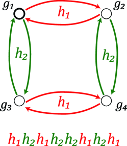
Figure 1: (color online) The Cayley graph $G(\mathcal{G},\Gamma)$ with $\mathcal{G}=\mathbb{Z}_{2}\otimes\mathbb{Z}_{2}=\{g_{i}\}_{i=1}^{4}=\{(0,0),(0,1),(1,0),(1,1)\}$ and $\Gamma=\{h_{1},h_{2}\}=\{g_{2},g_{3}\}=\{(0,1),(1,0)\}$ with an Eulerian path of length $L=8$ depicted. This group with the Cayley graph and the Eulerian cycle depicted here will be used in Sec. IV.3 to implement DCG constructions for the linear decoherence model.

This cycle can be associated to the control propagator $U_{\text{EDD}}(t)$ which describes evolution in $L$ consecutive intervals $I_{j}=[t_{j-1},t_{j}]$, that is,

$$U_{\text{EDD}}(t_{j})=F_{j}U_{\text{EDD}}(t_{j-1}),\;\;\;j=1,\ldots,L,$$ (19)

where $F_{j}$ is the group representation of the generator labeling the $j$-th edge in ${\cal C}$. According to Eq. (19), the control propagator follows the Eulerian path faithfully: The gating Hamiltonian $H_{\text{gate}}(t)$ varies in such a way that each evolution segment labeled by a generator $h_{j}$ along the path is implemented by a corresponding gate $F_{j}$. The evolution over $T_{c}=L\tau$ thus consists of each generator $F_{j}\in\Gamma$ being implemented precisely $d$ times. Suppose that the error associated with each gate $F_{j}$ is given by $\Phi_{F_{j}}$, determined by the manner in which $F_{j}$ is physically implemented:

$$\exp(-i\Phi_{F_{j}})=T_{+}\Big{[}\exp\Big{(}\!-i\int_{0}^{\tau}\!U_{\text{gate},j}(t)^{\dagger}H_{e}U_{\text{gate},j}(t)\Big{)}\Big{]},$$

where we have assumed that $F_{j}$ is generated through the application of a gating Hamiltonian $H_{\text{gate},F_{j}}(t)$ in the interval $[0,\tau]$ (which can be shifted forward in time), with

$$U_{\text{gate},j}(t)=T_{+}\Big{[}\exp\Big{(}\!-i\int_{0}^{t}\!H_{\text{gate},F_{j}}(s)ds\Big{)}\Big{]}.$$

The combined error associated with the EDD sequence can be approximated by a Magnus expansion [Eq. (15)]:

$$\Phi_{\text{EDD}}=\sum_{i=1}^{m}\Pi_{\mathcal{G}}(\Phi_{F_{i}})+\Phi_{\text{EDD}}^{[2+]},$$ (20)

with $\left\|\Phi_{\text{EDD}}^{[2+]}\right\|=O(\max_{j}\left\|\Phi_{F_{j}}\right\|^{2})$. In EDD, we require that the errors $\Phi_{F_{j}}$ associated with the control generators belong to the error set $\Omega_{e}$ corrected by $\mathcal{G}$. As long as this is the case, then $\Phi_{\text{EDD}}^{[1]}=0$ mod$B$, and the EDD sequence performs a noop with an asymptotically small error $\Phi_{\text{EDD}}^{[2+]}$ compared to the uncorrected evolution.

Given arbitrary linear decoherence, we will show in Sec. IV.3 how readily available control options for realizing the generators of ${\cal G}$ can produce errors that indeed belong to $\Omega_{e}$. For a generic open system, it need not be apparent which type of Hamiltonians and control inputs (if any) might be used to generate EDD generators such that their respective errors $\Phi_{F_{j}}$ are correctable by (some) ${\cal G}$, a question we refer to as the ‘gate permissibility problem’. To summarize, provided a set of permissible generator gates can be identified, EDD yields a constructive solution to our main problem as defined in Sec. II.2, with the desired target gate being the noop gate.

III.3 No-go theorem for black-box constructions

An important feature of EDD is that the net error given by Eq. (20) is canceled irrespective of how each gate $F_{j}$ representing a decoupling generator is implemented in terms of the control inputs, provided that (i) the same implementation is used each time $h_{j}$ appears along the path and (ii) each error $\Phi_{F_{j}}$ is correctable by ${\cal G}$. To state it differently, no a priori relationship between the errors $\{\Phi_{F_{j}}\}$ is assumed, as they cancel independently up to the first order [Eq. (20)]. In this sense, error correction in EDD is oblivious to the details of the control. Unfortunately, as we shall prove next, such ‘control-oblivious decoupling’ can only dynamically correct the noop gate.

Consider, specifically, a control sequence composed of $N$ gates $Q_{i}$ applied on $S$ in the presence of $H_{e}$. Ideally, let the sequence be intended to implement a gate $A=Q_{N}\cdots Q_{1}$. The EPG $\Phi_{Q_{i}}$ associated with $Q_{i}$ is assumed to be an arbitrary function of the gate $Q_{i}$:

$$\Phi_{Q_{i}}=\mathcal{E}(Q_{i}).$$

$\mathcal{E}$ depends in principle on $H_{e}$ as well as the details of implementation. Suppose, however, that as in EDD no information about such dependence is directly or indirectly incorporated into control design. We have the following:

Theorem. Consider a sequence of gates $A=Q_{N}Q_{N-1}\cdots Q_{1}$, and suppose that the combined first-order error $\Phi_{A}$ for this sequence is equal to zero mod$B$ as long as the individual errors $\Phi_{Q_{i}}$ belong to a subspace $\Omega_{e}\subseteq\Omega_{c}$ of dynamically correctable operators for all $i$. If no further assumptions are made on $\Phi_{Q_{i}}$, then the expectation values of operators in $\Omega_{e}$ are preserved by $A$.

Proof. Since no assumptions are made on $\Phi_{Q_{i}}$ (hence on $\Phi_{Q_{i}}$ mod$B$), the function $\mathcal{E}$ from unitary system operators into $\Omega_{e}$ is arbitrary. In particular, we may consider two error models defined by

$$\mathcal{E}_{1}(U)=X,\hskip 14.22636pt\mathcal{E}_{2}(U)=U^{\dagger}XU,$$

where $X$ is any operator in $\Omega_{e}$. Let $\Phi_{A,1}$ ($\Phi_{A,2}$) denote the combined error obtained under the error function $\mathcal{E}_{1}$ ($\mathcal{E}_{2}$). Let us define $P_{i}=Q_{i}\cdots Q_{1}$ for $N\geq i>0$ and $P_{0}=I_{S}$. From Eq. (15) and using the fact that $Q_{i}=P_{i}P_{i-1}^{\dagger}$, we have:

$$\Phi_{A,1}^{[1]} = \sum_{i=1}^{N}P_{i-1}^{\dagger}XP_{i-1}=0\text{ mod}B,$$ (21)

$$\Phi_{A,2}^{[1]} = \sum_{i=1}^{N}P_{i-1}^{\dagger}P_{i-1}P_{i}^{\dagger}XP_{i}P_{i-1}^{\dagger}P_{i-1}$$ (22)

$$= \sum_{i=1}^{N}P_{i}^{\dagger}XP_{i}=0\text{ mod}B.$$

Comparing Eq. (21) and Eq. (22) yields:

$$\forall X\in\Omega_{e}:P_{0}^{\dagger}XP_{0}-P_{N}^{\dagger}XP_{N}=X-A^{\dagger}XA=0\text{ mod}B.$$

We can write $X$ as $X=\tilde{X}+I_{S}\otimes B_{X}$ where $\text{Tr}_{S}\tilde{X}=0$ so that $\tilde{X}$ has no pure-bath component. The operator $A$ acts on the system only, thus we have

$$X-(A\otimes I_{B})^{\dagger}X(A\otimes I_{B})=0\text{ mod}B \Rightarrow \!\!\!\tilde{X}-A^{\dagger}\tilde{X}A=0$$

$$\Rightarrow \!\!\!X-A^{\dagger}XA=0$$

Clearly, $A\otimes I_{B}$ acts as identity on $\Omega_{e}$ and can generate no non-trivial dynamics on this subspace. $\blacksquare$

In other words, we may yet effect a control-oblivious unitary transformation on the system but it will necessarily commute with the subspace of errors that ${\cal G}$ can correct for, and will thus coincide with identity (noop) if the latter acts irreducibly on ${\cal H}_{S}$. Nonetheless, one might be interested in suppressing errors from a particular subset of more general errors. The No-Go theorem then still allows such a black-box solution to be viable for constructing primitive gates, as well as it allows to suitably combining DD with quantum encoding. For examples of constructions where decoherence is suppressed using BB pulses and the desired computational dynamics is encoded in a subspace or subsystem see Viola et al. (2000); Viola (2002); Khodjasteh and Lidar (2008); Lidar (2008).

From a practical standpoint, the No-Go theorem places restrictions on the ability to making fully portable DCGs where a fixed sequence of arbitrary implementations of gates effects a generic unitary gate on the system. In order to go beyond noop in constructing DCGs, we thus require to include certain specified gate implementations that circumvent the arbitrary EPG assumption.

IV Dynamically Corrected Gates beyond NOOP

A central point in EDD is that the combined EPG is determined by the variation of the control propagator between the gates at the vertexes of the Cayley graph underlying the scheme. In view of the above No-Go Theorem, identifying a procedure where an analogous error cancellation is achieved but a non-trivial target unitary is effected on $S$, requires access to relationships between errors associated to different gates. Identifying and exploiting such relationship is possible because both the algebraic structure of $H_{e}$ and the gating Hamiltonian are known. Thus, while the No-Go does not pose a fundamental obstacle for DQEC, it does complicate the design of robust control schemes and reduces their portability. It is the goal of this Section to provide explicit procedures for constructing and analyzing DCGs, by first illustrating the general approach and obtaining estimates of the uncorrected (higher than first-order) net error, and next providing full detail on linear decoherence- and dephasing- protected DCGs. Both for added clarity, and because the presence of a non-trivial $H_{S}\neq 0$ requires a system-dependent analysis, we take advantage in what follows of assumption (a2), that is, we explicitly let

$$H_{S}=0,\;\;H_{e}=H_{SB}+H_{B},\;\;H_{\text{gate}}(t)=H_{\text{ctrl}}(t),$$ (23)

and further discuss the role of $H_{S}$ in DQEC constructions in Sec. VI.

IV.1 DCG constructions and error estimates

Probably the simplest (albeit not unique) way to enforce the constraint of non-trivial gate error relationships is to imagine that two different gates share the same EPG to lowest order. Let $Q$ be the intended (primitive) target gate, with associated error $\Phi_{Q}$, and imagine that a special noop gate $I_{Q}$ is available, such that the error associated with $I_{Q}$ is also $\Phi_{Q}$:

$$U_{Q}=Q\,\exp(-i\Phi_{Q}),\;\;\;I_{Q}=I_{S}\,\exp(-i\Phi_{Q}).$$ (24)

That the above requirement can in fact be fulfilled will be addressed in Sec. IV.2. Assuming for now that Eq. (24) holds, consider attaching a self-directed edge $I_{Q}$ to each vertex on the Cayley graph $G(\mathcal{G},\Gamma)$, and let the Eulerian path ${\cal C}$ be modified so that the new edges added at each vertex are incorporated. The error associated with this new sequence (which clearly still acts as noop) is given, up to the first order, by

$$\Phi_{\text{DCG}}^{[1]}=\Phi_{\text{EDD}}^{[1]}+\Pi_{\mathcal{G}}(\Phi_{Q}),$$

and is canceled (mod$B$) as long as the errors $\Phi_{Q}$ and $\Phi_{F_{j}}$ belong to $\Omega_{e}$. Next, we change the final gate/edge $I_{Q}$ in the path we just created with the gate/edge $Q$ with error $\Phi_{Q}$. By construction, the error associated with the combined sequence remains unchanged, but the sequence now implements $Q$ as opposed to $I_{S}$. Thus, we have succeeded in obtaining a DCG that performs the desired gate $Q$ on $S$ with a smaller error as compared to its uncorrected implementation.

In line with the philosophy underlying DQEC approaches, the errors due to $H_{e}$ are suppressed asymptotically. This requires that the EPG of the primitive (uncorrected) gates be small to begin with in order to expect a relative improvement in DCG performance [recall Eq. (1)]. Even if this condition is met, the uncorrected errors associated with a large number of operations performed in succession tend to inevitably build up, thus additional precautions must be taken to avoid catastrophic error growth. Within FTQEC, this can still be prevented provided that DCG residual errors remain correctable by the given code architecture and smaller than the relevant threshold. This prompts us to estimate the uncorrected errors associated with DQEC constructions for each gate.

The asymptotic nature of DCG constructions rests on the validity of the Magnus expansion as an approximation of the effective Hamiltonian for short time intervals. When used to estimate the EPG associated with a gate $Q$ of duration $T=N\tau$, a sufficient condition is

$$\left\|H_{e}\right\|T<\pi,$$ (25)

where $N=1$ corresponds to a single primitive gate segment. Two remarks are in order. First, in view of assumption (c2), $\tau_{\text{min}}$ effectively limits the strength of error Hamiltonians that can be corrected using DCGs. Second, while including the environment Hamiltonian $H_{B}$ in $H_{e}$ has the advantage of simplicity, the resulting convergence radius (time) for the Magnus expansion tends to be overly pessimistic in this way, in particular it may grossly overestimate the error in the case where $\left\|H_{B}\right\|\gg\left\|H_{SB}\right\|$. One solution is to move to a toggling frame that removes the evolution of $B$. We refer for instance to Khodjasteh and Lidar (2007) for an analysis along this lines, yielding a tighter convergence radius for the Magnus expansion, $\left\|H_{SB}\right\|T<\pi$.

The uncorrected errors that do not cancel as a result of a DQEC protocol can be bounded by the second- and higher- order contributions to the Magnus series Not (a). Recalling Eq. (12), we can estimate the uncorrected error $\Phi_{Q,\text{DCG}}$ associated with a DCG $Q$ as

$$\left\|\Phi_{Q,\text{DCG}}^{[2+]}\right\| \!=\! \frac{1}{2}\left\|\int_{0}^{T}\int_{0}^{t_{2}}[H_{e}(t_{1}),H_{e}(t_{2})]dt_{1}dt_{2}\right\|$$

$$\!\leq\! \frac{T^{2}}{4}\max_{t_{1}<t_{2}}\left\|\,[H_{e}(t_{1}),H_{e}(t_{1})]\,\right\|$$

$$\!\leq\! \frac{T^{2}}{4}\Big{(}2\,\left\|H_{B}\right\|\left\|H_{SB}\right\|+\left\|H_{SB}\right\|^{2}\Big{)},$$

where we have used the unitary invariance properties of $\left\|\cdot\right\|$. While Eq. (IV.1) gives an upper bound for the uncorrected error associated with any gate $Q$ for which $\Phi_{Q}^{[1]}=0$ mod$B$, it fails to capture many interesting features of the interplay between the pure environment evolution and the system-bath coupling. We will reconsider the latter numerically in the specific setting of Sec. V.

Note that the first order error $\Phi_{Q}^{[1]}$ associated with a primitive gate $Q$ (not corrected through DQEC) will naturally depend on the number of qubits $n$ in the system. For the linear decoherence model we have

$$\left\|\Phi_{Q}^{[1]}\right\|\propto n,$$

thus the EPG per qubit is expected to be constant (size-independent) up to the first order. For DCGs, the first order error is zero, and to obtain a dependence on the $n$, we need to focus on $\Phi_{Q,\text{DCG}}^{[2]}$, estimated above. Using Eq. (IV.1), we may write

$$\left\|\Phi_{Q,\text{DCG}}^{[2+]}\right\|=O(n^{s}),\;\;\;1\leq s\leq 2.$$

The upper bound is given by $\left\|H_{SB}\right\|^{2}$ [Eq. (IV.1)], whereas the lower bound is achieved, for example, when the bath operators $B_{\alpha}^{(i)}$ act locally, $[B_{\alpha}^{(i)},B_{\beta}^{(j)}]\propto\delta_{i,j}$, for all $\alpha,\beta$.

IV.2 Finding gates with same error

As described in Sec. IV.1, a fundamental ingredient in DCGs is that two control sequences are found for every desired gate $Q$: One designated to perform a noop and the other designated to perform $Q$, such that the corresponding errors are equal up to the first order. We now give a simple method for generating such sequences, which in the language of Ref. Khodjasteh and Viola, 2009b realize a so-called first-order balance pair.

Suppose that a given control input $h_{\alpha}^{Q}(t)$ is intended to produce a unitary gate $Q$ during an interval $[0,\tau]$, and let $H_{\text{gate}}^{Q}$, and $U_{\text{gate}}(t)$ denote the gating Hamiltonian and corresponding propagator for $Q$ over $t\in[0,\tau]$, respectively. The error associated with $Q$ is given by

$$\exp(-i\Phi_{Q}) \!=\! T_{+}\Big{[}\exp\Big{(}\!-i\int_{0}^{\tau}\!H_{e}(s,0)ds\Big{)}\Big{]},$$

with $H_{e}(t,0)$ being the toggling frame error Hamiltonian as in Eq. (12). We next smoothly extend the control profile for $Q$ to $[0,2\tau]$ by applying a gate $Q^{\prime}$ immediately after $Q$, in such a way that the overall control propagator for $t\in[0,2\tau]$ is given by:

$$U^{\prime}_{\text{gate}}(t,0)=\left\{\begin{array}[]{ll}U_{\text{gate}}(t),&0<t<\tau;\text{ gate }Q,\\ U_{\text{gate}}(2\tau-t),&\tau<t<2\tau;\text{ gate }Q^{\prime}.\end{array}\right.$$

The extended (composite) gate $I_{Q}=Q^{\prime}Q$ implements the identity (noop), with a first-order error given by:

$$\Phi_{Q^{\prime}Q}^{[1]} = \int_{0}^{2\tau}U^{\prime}_{\text{gate}}(t,0)^{\dagger}H_{e}U^{\prime}_{\text{gate}}(t,0)dt$$

$$= 2\int_{0}^{\tau}U_{\text{gate}}(t)^{\dagger}H_{e}U_{\text{gate}}(t)dt=2\,\Phi_{Q}^{[1]}.$$

Consider next another control propagator associated with a gate $Q_{1/2}$ over the interval $[0,2\tau]$ obtained by letting

$$U^{\prime\prime}_{\text{gate}}(t,0)=U_{\text{gate}}(t/2),\;\;\;0<t<2\tau.$$

The first-order error associated with $Q_{1/2}$ reads

$$\Phi_{Q_{1/2}}^{[1]} = \int_{0}^{2\tau}U^{\prime\prime}_{\text{gate}}(t,0)^{\dagger}H_{e}U^{\prime\prime}_{\text{gate}}(t,0)dt$$

$$= 2\int_{0}^{\tau}U_{\text{gate}}(t)^{\dagger}H_{e}U_{\text{gate}}(t)dt=2\,\Phi_{Q}^{[1]}.$$

By comparing Eqs. (IV.2)-(IV.2), we observe that while $Q^{\prime}Q$ ideally implements the identity and $Q_{1/2}$ implements $Q$, the EPGs resulting from $H_{e}\neq 0$ are equal up to the first order.

Given enough control over the $\{h_{\alpha}(t)\}$, simple recipes may be given for implementing both $Q^{\prime}$ and $Q_{1/2}$. For instance, $Q^{\prime}$ may be realized by applying $-h_{\alpha}^{Q}(t-\tau)$ (the reverse anti-symmetric profile to $h_{\alpha}^{Q}(t)$) when $t>\tau$, see Fig. 2.

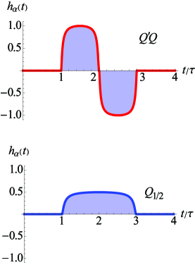
Figure 2: (color online) Control profiles for implementing two gates $I_{Q}=Q^{\prime}Q$ and $Q_{1/2}$, that correspond to a target identity gate and a target gate $Q$, with equal first-order error.

Likewise, to implement $Q_{1/2}$, we may use a control input $h_{\alpha}^{Q_{1/2}}(t)$ such that $\int_{0}^{t}h_{\alpha}^{Q_{1/2}}(s)ds=\int_{0}^{t/2}h_{\alpha}^{Q}(s)ds$. For example, if the pulse profiles are rectangular, $Q_{1/2}$ may be generated by using a control input with half the speed and half the strength of the one used for $Q$. The two prescriptions so obtained for $QQ^{\prime}$ and $Q_{1/2}$ corresponds then, respectively, to the piecewise-constant profiles given in Eqs. (4)-(5) of Khodjasteh and Viola (2009a). If we assume that all primitive gates have the same duration $\tau$, then the number of primitive gates required in each DCG will be $dm+2d=d(m+2)$ [recall Sec. IV.1].

The construction described in this section should, in its simplicity, mainly be taken as a proof-of-concept illustration of how to meet the fundamental ‘same error requirement’ of Eq. (24). In practice, numerical optimization techniques may prove either helpful or indispensable, especially in the presence of additional control-input constraints. For example, if negative control inputs are not available to implement the required balance pair $(I_{Q},Q_{*})$ as $(Q^{\prime}Q,Q_{1/2})$, we can invoke a more general construction given in Khodjasteh and Viola (2009b). The latter only assumes access to stretchable control profiles to implement $(I_{Q},Q_{*})$, with a resulting sequence that is longer by a factor of $3/2$ with respect to $(Q^{\prime}Q,Q_{1/2})$. The important point, however, is that any DCG construction necessitates a recipe for the control inputs that will logically produce a non-trivial relationship among the corresponding EPGs, in order to evade the No-Go theorem of Sec. III.3.

IV.3 Permissible controls for general linear decoherence and pure dephasing

We next specialize the above general constructions to two physically relevant error models on $n$ (driftless) qubits: (i) the generic linear decoherence model described by Eq. (5), where $\Omega_{e}=\Omega_{e}^{\{1\}}$ includes arbitrary single-qubit error operators, Eq. (6); (ii) the pure dephasing (or single-axis decoherence) model, which is formally obtained from the above generic case by assuming that coupling to $B$ occurs along a known direction, say $Z$, in which case $B_{\alpha}^{(i)}=0$ for $\alpha=1,2$. We will refer to the resulting subspace of system-bath error operators,

$$\Omega_{e}=\text{span}\{Z^{(i)}\otimes B_{z}^{(i)}\}\equiv\Omega_{e}^{Z},$$ (30)

as the ‘(pure) phase errors’. The dephasing model is a common approximation often used in situations where a quantization axis defines the internal states of the individual qubits (such as in standard NMR QIP settings Cor ), and allows for significantly less resource-intensive FTQEC schemes to be devised in comparison to general linear decoherence Aliferis and Preskill (2008). This is not only due to the fact that the errors involved in dephasing are inherently restricted, but also to the fact that the algebraic structures associated with their growth are much simpler Not (b).

IV.3.1 One- and two-body controllable Hamiltonians

Within the network model of QC, the majority of proposals invoke the use of control Hamiltonians that act non-trivially on single or pairs of qubits. Let us consider the set of primitive gates which are generated by switching on and off control input in a control Hamiltonian parametrized as follows:

$$H_{\text{ctrl}}(t) = H_{\text{ctrl}}^{(\text{pair})}(t)+H_{\text{ctrl}}^{(\text{single})}(t),$$ (31)

$$H_{\text{ctrl}}^{(\text{single})}(t) = \sum_{i=1}^{n}\sum_{\alpha=X,Y}h_{\alpha}^{(i)}(t)S_{\alpha}^{(i)},$$

$$H_{\text{ctrl}}^{(\text{pair})}(t) = \sum_{i\neq j}\sum_{\alpha=1}^{3}h_{\alpha\alpha}^{(ij)}(t)S_{\alpha}^{(i)}S_{\alpha}^{(j)},$$

where we generally allow for homogeneous two-body interactions which include natural entangling Hamiltonians such as the Ising $(ZZ)$ and Heisenberg $(\mathbf{S}\cdot\mathbf{S}\equiv XX+YY+ZZ)$ interactions. We will focus on primitive gates during which the control propagator can be expanded as

$$U_{\text{ctrl}}(t,0) = \exp\left[-iA^{\{1\}}(t)-iA^{\{2\}}(t)\right],$$ (32)

$$A^{\{1\}}(t) = \sum_{i=1}^{n}\sum_{\alpha=1}^{3}\theta_{\alpha}^{(i)}(t)S_{\alpha}^{(i)},$$

$$A^{\{2\}}(t) = \sum_{i<j}\sum_{\alpha=1}^{3}\theta_{\alpha}^{(i,j)}(t)S_{\alpha}^{(i)}S_{\alpha}^{(j)},$$

where the functions $\theta_{\alpha}^{(i)}(t)$, $\theta_{\alpha}^{(i,j)}(t)$ are suitable control integrals and the set of qubits involved in two-qubit control has no intersection with the set of qubits involved in single-qubit control. That is, we require that

$$\{i|\theta_{\alpha}^{(i)}(t)\neq 0\}\cap\{j|\theta_{\alpha}^{(k,j)}(t)\neq 0\}=\emptyset,$$ (33)

so that $A_{\{1\}}(t)$ and $A_{\{2\}}(t)$ commute. For example, applying a $ZZ$ Hamiltonian between qubits 1 and 2, while qubits 3, 4, and 5 are affected by single-qubit Hamiltonians is an example where the above constraint is naturally obeyed. Note that such a ‘divided control’ is implicit in the circuit model of QC where gates are applied in parallel only when they commute. We emphasize that unless certain commutativity conditions are satisfied, in general $\theta_{\alpha}^{(ij)}(t)\neq\int_{0}^{t}h_{\alpha}^{(ij)}(s)ds$, and a linear relationship among the control inputs does not translate into a linear relationship among the control integrals.

IV.3.2 Error-corrected gate constructions

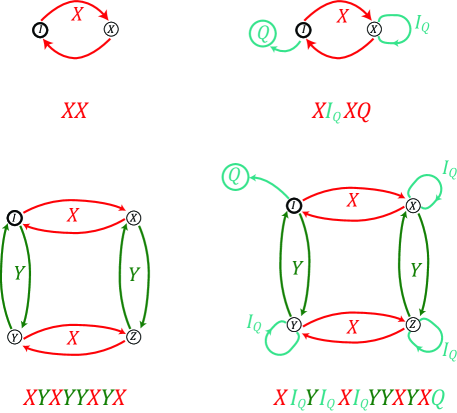
Figure 3: (color online) Left: Cayley graphs for $\mathbb{Z}_{2}$ (top) and $\mathbb{Z}_{2}\otimes\mathbb{Z}_{2}$ (bottom), relevant to pure dephasing and arbitrary linear decoherence, respectively. Representative Eulerian cycles and the corresponding EDD sequences are depicted. Right: Modified Cayley graphs for DCG constructions based on $\mathbb{Z}_{2}$ (top) and $\mathbb{Z}_{2}\otimes\mathbb{Z}_{2}$ (bottom), respectively. Relevant Eulerian paths and the corresponding DCG sequences are depicted.

A good (minimal) DD group for the error set $\Omega_{e}^{\{1\}}$ corresponding to arbitrary linear decoherence is given by

$$\Omega_{e}^{\{1\}}\rightarrow\mathcal{G}_{\text{LD}}=\mathbb{Z}_{2}\otimes\mathbb{Z}_{2},$$

represented in ${\cal H}_{S}=({\mathbb{C}}^{2})^{\otimes n}$ through the $n$-fold tensor power representation $\{S_{\alpha}^{(\text{all})}\}=\{I_{S},X^{(\text{all})},Y^{(\text{all})},Z^{(\text{all})}\}$ Viola et al. (1999a); Viola and Knill (2003). $\mathcal{G}_{\text{LD}}$ has two generators, which under the above representation we may take to be $\{F_{j}\}=\{X^{(\text{all})},Y^{(\text{all})}\}$. Observe that the subspace of operators decoupled by $\mathcal{G}_{\text{LD}}$ is not limited to $\Omega_{e}^{\{1\}}$, as it includes, for example, inhomogeneous bilinear couplings of the form $S_{\alpha}^{(i)}S_{\beta}^{(j)}$, with $i\neq j$ and $\alpha\neq\beta$. Thus, $\Omega_{c,\text{LD}}\supset\Omega_{e}^{\{1\}}$, which allows a wider class of primitive gates to be corrected using $\mathcal{G}_{\text{LD}}$ than the noop gate with single-qubit errors as originally analyzed in Viola and Knill (2003).

The DD group for pure phase errors is simpler:

$$\Omega_{e}^{Z}\rightarrow\mathcal{G}_{Z}=\mathbb{Z}_{2},$$

represented via $\{I_{S},X^{(\text{all})}\}$, and with the single generator $\{F\}=\{X^{(\text{all})}\}$. Notice again that this representation also decouples errors beyond the simple dephasing terms, for instance inhomogeneous error operators of the form $Z^{(i)}X^{(j)}$ with $i\neq j$, therefore again we have $\Omega_{c,\text{Z}}\supset\Omega_{e}^{\{Z\}}$. A pictorial view of the Cayley graphs relevant to both error models under examination is given in the left panels of Fig. 3, along with representative Eulerian cycles.

A possible EDD sequence for correcting noop under the general decoherence model is given by:

$$\text{EDD}^{\text{lin}}\rightarrow X^{(\text{all})}Y^{(\text{all})}X^{(\text{all})}Y^{(\text{all})}Y^{(\text{all})}X^{(\text{all})}Y^{(\text{all})}X^{(\text{all})},$$ (34)

where operations are understood to be applied from right to left, following the underlying Eulerian cycle. This implies a total number of $md=4(\text{group elements})(2\text{ generators})=8$ gates. Similarly, EDD under pure dephasing may be implemented by the sequence:

$$\text{EDD}^{\text{Z}}\rightarrow X^{(\text{all})}X^{(\text{all})},$$ (35)

which consists of just $md=2$ gates, and may be viewed as implementing a form of ‘continuous-time’ spin-echo Viola (2004); Nir . The relevant DCG constructions are based on modifications of the above EDD gate sequences. Let $Q$ denote a primitive gate. We define $I_{Q}=QQ^{\prime}$ and $Q_{1/2}$ using the constructions of Sec. IV.2. For general linear decoherence, a DCG for $Q$ is then given by:

$$\text{DCG}^{\text{lin}}\rightarrow Q_{1/2}X^{(\text{all})}Y^{(\text{all})}X^{(\text{all})}Y^{(\text{all})}I_{Q}Y^{(\text{all})}I_{Q}X^{(\text{all})}I_{Q}Y^{(\text{all})}I_{Q}X^{(\text{all})}.$$ (36)

Similarly, for pure dephasing, we simply have:

$$\text{DCG}^{\text{Z}}\rightarrow Q_{1/2}X^{(\text{all})}I_{Q}X^{(\text{all})}.$$ (37)

The sequences given in Eqs. (36)-(37) represent Eulerian paths in the modified Cayley graphs corresponding the DD groups $\mathcal{G}_{\text{LD}}$ and $\mathcal{G}_{Z}$, obtained as described in Sec. IV.1; see also right panels in Fig. 3. If all primitive gates have the same duration $\tau$, since each added ‘arm’ in the modified graph has duration $2\tau$, the resulting time overheads may be summarized as follows:

	Linear decoherence	Pure dephasing
EDD	8	2
DCG	16	6

IV.3.3 Error per gate structure

In order for the DQEC constructions just provided to be valid, it is necessary to explicitly show that the errors associated with the primitive gates generated from the (divided) one- and two-body Hamiltonians of Sec. IV.3.1 can indeed be decoupled by the appropriate DD group.

Consider linear decoherence and $\mathcal{G}_{\text{LD}}$ first. Let the control propagator for a primitive gate $Q$ be given by Eq. (32). The toggling frame error Hamiltonian $H_{e}(t)$ [Eq. (12)] is given by

$$H_{e}(t) = e^{i[A^{\{1\}}(t)+A^{\{2\}}(t)]}H_{e}e^{-i[A^{\{1\}}(t)+A^{\{2\}}(t)]}$$

$$= e^{iA^{\{2\}}(t)}e^{iA^{\{1\}}(t)}H_{e}e^{-iA^{\{1\}}(t)}e^{-iA^{\{2\}}(t),}$$

where we used the fact that $[A^{\{1\}}(t),A^{\{2\}}(t)]=0$. Notice next that $\exp\left[iA^{\{1\}}(t)\right]H_{e}\exp\left[-iA^{\{1\}}(t)\right]$ can be expanded as a sum of single-qubit terms up to the first order Magnus, thus

$$e^{iA^{\{1\}}(t)}H_{e}e^{-iA^{\{1\}}(t)}=\sum_{\alpha,i}S_{\alpha}^{(i)}\otimes C_{\alpha}^{(i)}\equiv F_{e}(t)\in\Omega_{e}^{\{1\}}.$$

Up to the first order we may then write:

$$\Pi_{\mathcal{G}_{\text{LD}}}[H_{e}(t)]=e^{iA^{\{2\}}(t)}\Pi_{\mathcal{G}_{\text{LD}}}[F_{e}(t)]e^{-iA^{\{2\}}(t)}=0\mbox{ mod$B$,}$$

where we used the fact that $[e^{iA^{\{2\}}(t)},S_{\alpha}^{(\text{all})}]=0$. Subsequently, the first-order error $\Phi_{Q}^{[1]}$ is decoupled by $\mathcal{G}_{\text{LD}}$:

$$\Pi_{\mathcal{G}_{\text{LD}}}(\Phi_{Q}^{[1]})=\Pi_{\mathcal{G}_{\text{LD}}}\Big{(}\int_{0}^{t}H_{e}(s)ds\Big{)}=0\mbox{ mod$B$,}$$

which establishes the desired error cancellation.

For the pure dephasing model, the set of allowed control Hamiltonians in DCGs is slightly more restricted. For example, consider a DCG construction based on Eq. (37), where $\mathcal{G}_{Z}$ is represented by $\{I,X^{(\text{all})}\}$. In this case, the single-qubit control Hamiltonians used in $Q$ cannot include $Y^{(i)}$ terms as they would result in errors that are not decoupled by this particular representation. However, one can alternatively use the representation $\{I,Y^{(\text{all})}\}$ of $\mathcal{G}_{Z}$, if the control Hamiltonians used in $Q$ are given by $Y^{(i)}$. The choice of the particular representation of $\mathcal{G}$ used in constructing DCGs may thus affect the set of permissible Hamiltonians. While this is not surprising in view of existing results on control of decoupled evolutions Viola et al. (1999b), analyzing in full generality the compatibility of primitive gate sets with DQEC strategies for a given error model of interest warrants a separate investigation.

V Case study: Dynamical correction of spin-bath decoherence

In this section, we specialize the system-independent analytic DCG constructions described in Sec. IV to the paradigmatic setting of spin-bath decoherence. While quantitative modeling of a specific device is not our purpose here, our analysis is inspired by spin-based QIP architectures – in particular, electron spin qubits in semiconductor quantum dots, as considered for instance in Refs. Loss and DiVincenzo, 1998; Hanson et al., 2007; Zhang et al., 2007a. In which physical parameter regime(s) is the improvement predicted for DQEC methods actually to be seen? What distinctive physical features and performance trade-offs are associated with DCG constructions? Beside complementing and expanding our previous numerical results Khodjasteh and Viola (2009a), these are two questions that the present investigation further addresses by example.

V.1 Model system and primitive gates

Let the system $S$ consist of $n$ individually addressable spin-$1/2$ degrees of freedom, and let the environment $B$ likewise consist of $n_{B}$ spin-$1/2$ particles. If we denote by $\mathbf{I}^{(i)}$ the spin vector operator associated with the $i$-th bath particle, the internal Hamiltonian $H_{\text{int}}=H_{B}+H_{SB}$ we consider reads:

$$H_{B} = \sum_{1\leq i<j\leq n_{B}}\Gamma_{i,j}(\mathbf{I}^{(i)}\cdot\mathbf{I}^{(j)}-3I_{Z}^{(i)}I_{Z}^{(j)}),$$

$$H_{SB} = \sum_{i=1}^{n}\sum_{k=1}^{n_{B}}A_{k}^{(i)}\mathbf{S}^{(i)}\cdot\mathbf{I}^{(k)}.$$

Physically, $H_{B}$ describes dipolar interactions between the bath spins, whereas $H_{SB}$ describes a (hyperfine) contact interaction of each qubit with the bath. For concreteness, we further assume in what follows that the coupling strength $\Gamma_{i,j}$ between bath spins $i$ and $j$ is arbitrarily chosen from a uniform random distribution in $[-\Gamma,\Gamma]$, and similarly that the hyperfine coupling strengths $A_{k}^{(i)}$ for each qubit are independently sampled uniformly at random from the $[-A,A]$ interval.

In line with Eq. (31), control over individual qubits and pairs of qubits is introduced through a gating Hamiltonian of the form

$$H_{\text{gate}}(t)=\sum_{i=1}^{n}\sum_{\alpha=X,Y}h_{\alpha}^{(i)}(t)S_{\alpha}^{(i)}+\sum_{i,j=1}^{n}h_{W}^{(i,j)}(t)\mathbf{S}^{(i)}\cdot\mathbf{S}^{(j)},$$

where $\mathbf{S}^{(i)}\cdot\mathbf{S}^{(j)}$ is the Heisenberg exchange interaction Not (c). Thus, each primitive gate is realized by switching the control parameters $h_{X}^{(i)}(t)$, $h_{Y}^{(i)}(t)$, and $h_{W}^{(i,j)}(t)$, under the ‘divided control’ assumption of Eq. (33). In particular, we can simply assume that at each time $t$ the qubits controlled through $X^{(i)}$, $Y^{(i)}$, and $\mathbf{S}^{(i)}\cdot\mathbf{S}^{(j)}$ are distinct, and use as a starting point for DQEC the universal set of primitive gates given by ideal gates $\{\exp(-i\theta C)\}$, where $C$ can be $X^{(i)}$, $Y^{(i)}$, and $\mathbf{S}^{(i)}\cdot\mathbf{S}^{(j)}$. We restrict available control inputs to the simplest choice of rectangular profiles: thus, a primitive gate is simply achieved by turning on the corresponding control input for a duration $\tau$ at a fixed strength $h$, allowing any control Hamiltonian to be written as a piece-wise constant function of time. The choice of the rectangular profiles allows for numerically exact simulations Not (d), while avoiding inessential complications in describing relevant control constraints and imperfections. In particular, the bounded-strength control constraint (c1) translates into demanding that $\text{max}_{t}\left|h_{Q}(t)\right|<h_{\text{max}}$, while the constraint (c2) implies a shortest gating time $\tau\geq\tau_{\text{min}}$ [Sec. II.2]. As an illustrative example of control errors, we may define over-rotation errors by replacing the nominal rotation angle $2\theta$ in each (piece-wise constant) control segment with $2\theta(1+\varepsilon)$. If $\varepsilon$ fluctuates non-deterministically over different instances of a particular gate, we have a random over-rotation; a constant (realization-independent) $\varepsilon$ defines a systematic over-rotation.

Within the above setting, the internal Hamiltonian is the error Hamiltonian, $H_{e}=H_{\text{int}}$ and, as remarked, there is no drift, $H_{S}=0$. Since $H_{SB}$ belongs to $\Omega_{e}^{\{1\}}$, as described in Sec. III the relevant DD group $\mathcal{G}_{\text{LD}}$ discussed in IV.3.2. Note that the DD problem for a single electron-spin qubit in contact with a nuclear-spin bath has been extensively analyzed using BB pulses in Zhang et al. (2007b, c, 2008), the limit $H_{S}\approx 0$ corresponding to the low-bias regime where transverse and longitudinal relaxation fully compete. In our case, the two available group generators are realized through collective spin-flip gates, and the DCG constructions of Sec. IV.1 may be used. Thus, a primitive gate $Q=\exp(-i\theta C)$ of duration $\tau$ is converted to a DCG gate through the following control Hamiltonian:

$$H_{\text{DCG}}(t)=\begin{cases}H_{i},&t\in[(i-1)\tau,i\tau]\text{, }i=1,\cdots,16,\\ 0&t\notin[0,16\tau],\end{cases}$$ (38)

where explicitly we have (cf. also the DCG circuit given in Fig. 1 of Khodjasteh and Viola (2009a)):

$$H_{i}=\frac{1}{\tau}\begin{cases}\frac{\pi}{2}\left(X^{(1)}+\cdots+X^{(n)}\right),\,&i=1,7,12,14,\\ \frac{\pi}{2}\left(Y^{(1)}+\cdots+Y^{(n)}\right),\,&i=4,10,11,13,\\ +\theta C,&i=2,5,8,\\ -\theta C,&i=3,6,9,\\ +\frac{\theta}{2}C,&i=15,16.\end{cases}$$

Notice that besides the original primitive gate $Q$ used in segments $i=2,5,8$, in segments $i=3,6,9$ we implement the gate $Q^{-1}$ (needed for the special noop gate $I_{Q}$) through negative control inputs, while $Q_{1/2}$ in segments $i=15,16$ is obtained by using half the control power than for $Q$.

V.2 Numerical results

Perhaps the most important and obvious question, if DCGs are to be incorporated in a QC architecture, is whether they can usefully improve EPGs. While in theory DCG constructions are provably effective in the asymptotic limit of small errors, how stringent in practice this limit might be, can sensitively depend upon the specifications and operating constraints of the device technology at hand. For this reason, quantitative predictions on the effectiveness of DCGs are thus best formulated and addressed having a specific experimental platform in mind. Numerical simulations in toy models as we examine can yet be instrumental in developing intuition on how to map out the actual regime of improvement as different parameters are varied – in preparation for realistic scenarios where both $H_{SB}$ and $H_{B}$ are typically fixed by either physical or fabrication constraints.

In the numerical analysis that follows, we explore a wide range of open-system as well as control parameters, specifically $A$, $\Gamma$, and the base gate interval $\tau$, which for the current purpose can be also thought as identifying the shortest accessible modulation timescale, $\tau\equiv\tau_{\text{min}}$. In order to allow for arbitrary precision matrix calculations (see also the Appendix), we focus on a relatively small open system, letting $n=2$, $n_{B}=6$ henceforth. In all simulations, the qubit register is initialized in the fixed reference state $|\psi_{\text{in}}\rangle=({\left|00\right\rangle+\left|01\right\rangle}/{\sqrt{2}})$, whereas the environment is initially maximally mixed, $\rho_{B}^{\text{in}}=I_{B}/2^{n_{B}}$. The evolution of the combined density matrix for the system and the environment is then calculated by multiplying exact matrix exponentiation for piecewise constat Hamiltonians describing the segments of the evolution. As representative target quantum gates, we consider single- and two-qubit rotations by $\pi/4$, that is:

$$R_{\pi/4}^{(1)}=\exp[-i\,({\pi}/{8})X^{(1)}]\otimes I^{(2)},$$

$$W_{\pi/4}^{(1,2)}=\exp[-i\,({\pi}/{8})\mathbf{S}^{(1)}\cdot\mathbf{S}^{(2)}]\equiv\sqrt{\textsc{swap}},$$

where the last equality makes explicit contact with the (universal) square-root-of-swap gate Nielsen and Chuang (2000); Loss and DiVincenzo (1998). Both the (first-order) improvement ratio introduced in Eqs. (2)-(3), $r^{[1]}\equiv r$, or directly the corresponding (in)fidelity contributions for the given initial state, will be used as a metric for quantifying DCG performance.

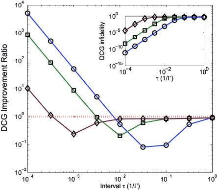
Figure 4: (color online) Improvement ratio as a function of (minimum) gating interval $\tau$, for the two-qubit target gate $W_{\pi/4}^{(1,2)}$. The ‘no improvement’ (horizontal) line $r=1$ is included for reference in this and all other figures that use $r$ as a metric for performance. The internal-bath Hamiltonian is kept fixed at $\Gamma=1$, whereas $A/\Gamma$ takes the value $10^{2}$ [brown diamonds], $10^{1}$ [green squares] and $1$ [blue circles]. Inset: Infidelity error for the corresponding DCG implementation, $1-f_{W_{\text{DCG}}}$, as a function of $\tau$, for the same parameters used in the main panel.

We first focus on the case of perfect control ($\varepsilon=0$). Representative results on the dependence of the improvement ratio $r$ upon the (minimum) gating interval $\tau$ are depicted in Fig. 4, where the above $W_{\pi/4}^{(1,2)}$ gate is considered for a fixed realization of the dipolar-bath Hamiltonian $H_{B}$ Rea . Weak- to strong- coupling decoherence regimes are then probed by varying the ratio $A/\Gamma$. All curves demonstrate the expected improvement in the limit of sufficiently small $\tau$. Different features are worth highlighting: first, as $\tau\rightarrow 0$, the data are consistent with the quadratic scaling with $1/\tau$ expected from Eq. (3) (for $A=1$, for instance, a fit of $\log(r)$ vs. $\log(\tau)$ yields $1.9991\pm 0.0002$). Emergence of such a scaling may be taken as a good indication that asymptotic conditions are well obeyed by the implementation. Second, the minimum gate interval $\tau=\tau^{\ast}(A;\Gamma)$, at which the improvement region for DQEC ($r>1$) is entered as $\tau$ is decreased, depends on the system-bath coupling strength – a larger $A$ (stronger decoherence) requires shorter values of $\tau^{\ast}$ to be accessed in order for DQEC to be effective, as intuitively expected. Note that, qualitatively, a dependence of $r$ upon both $H_{SB}$ and $H_{B}$ is expected on the basis of the uncorrected error associated with a DCG, Eq. (IV.1). Only in the limit where $\Gamma\rightarrow 0$ (a so-called ‘non-dynamical’ bath Zhang et al. (2007b, 2008)) does the first-order improvement regime simply relate to the coupling strength $\left\|H_{SB}\right\|$, which is fixed through $A$.

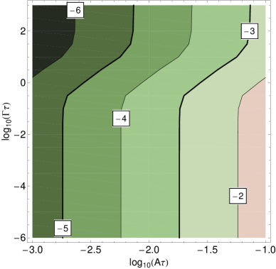
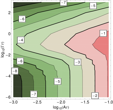
Figure 5: (color online) Iso-fidelity contour plots for the implementation of the single-qubit target gate $R_{\pi/4}^{(1)}$ for fixed (minimum) gating time $\tau=1$. Top: Primitive uncorrected implementation. Bottom: DCG implementation. In both cases, the integers labeling each curve give (the logarithm of) the corresponding infidelity error, with darker colors corresponding to higher fidelity values.

Exploring the interplay between $H_{SB}$ and $H_{B}$ as they are simultaneously varied for fixed (finite) values of the gating interval $\tau$ reveals additional interesting structure, as shown in Fig. 5. In particular, the loss of fidelity of a primitive single-qubit gate (top panel) is contrasted to the loss of fidelity of the corresponding DCG version (bottom panel) over a range of intra-bath and system-bath couplings, $\Gamma$ and $A$, respectively. Neither the uncorrected nor the DCG gate implementations depend in a similar manner upon the two parameters, the asymmetry in behavior being ‘amplified’ by the DCG. As a first interesting feature, only a mild dependence upon $\Gamma$ is observed for primitive gates implementations, the corresponding fidelity increasing for very strong intra-bath dynamics. This effect can be partly understood if, as mentioned in Sec. IV.1, $H_{B}$ is included in the definition of the toggling frame: A very strong $H_{B}$ will then induce fast oscillations in $H_{e}(t)$, resulting in smaller EPGs [cf. Eq. (12)]. Secondly, and more interestingly, a non-monotonic behavior emerges for DCG implementations as the intra-bath coupling $\Gamma$ is varied.

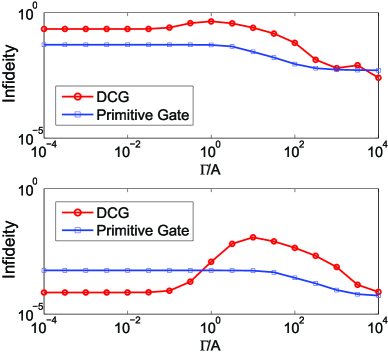
Figure 6: (color online) Infidelity, $1-f$, as a function of intra-bath/system-bath coupling scales for implementing the single-qubit gate $R_{\pi/4}^{(1)}$, at fixed $A=1$. Primitive vs DCG implementations are contrasted for two different gating times $\tau=0.1$ (top) and $\tau=0.01$ (bottom).

The dependence of fidelities for DCG and primitive gates on $H_{B}$ through $\Gamma$ is further highlighted in Fig. 6, where two representative values of $\tau$ are examined. The resonance-like behavior in the DCG patterns is evident, even when no significant improvement is expected. DQEC strategies such as DD or DCGs thus may probe the strength of the internal bath dynamics $H_{B}$, making them potentially attractive as a diagnostic tool for complex non-Markovian open quantum systems.

Besides the error effects associated with $H_{SB}$ and $H_{B}$, it is instructive to explore the impact of classical control errors in our setting, for example focusing on overrotation errors in the single-qubit gate $R_{\pi/4}^{(1)}$. As further discussed in Sec. VI.1 below, two different models for control imperfections may be physically relevant: (i) The nominal control Hamiltonian may be modified through the addition of a ‘deviation’ Hamiltonian with a fixed strength, $H^{\prime}_{\text{gate}}(t)=H_{\text{gate}}(t)+\varepsilon H_{\text{dev}}$, where $H_{\text{dev}}$ is a Hermitian operator with units of energy and $\varepsilon$ a small number (recall that $H_{\text{gate}}(t)=H_{\text{ctrl}}(t)$ as long as $H_{S}=0$). This results in a scaled systematic EPG, that can be tolerated (to first order) DCG constructions, similar to the errors due to the bath. (ii) The nominal control Hamiltonian may be systematically scaled by a factor:

$$H^{\prime}_{\text{gate}}(t)=(1+\varepsilon)H_{\text{gate}}(t).$$ (39)

This results in a fixed systematic EPG, in the sense that even in the absence of the bath, a control segment of duration $\tau$ intended to produce $\exp(-i\theta C)$ will instead implement $\exp[-i\theta(1+\varepsilon)C]$, regardless of $\tau$. In the simulations, model (ii) is implemented, given that there is no a priori indication that such errors should be tolerated by DCGs, unlike errors of type (i).

Illustrative results for the DCG improvement ratio $r$ obtained for a non-dynamical bath ($\Gamma=0$) at fixed $A=1$ are summarized in Fig. 7, as a function of the gating interval and for different values of the control error strength. Overall, although the observed performance remains fairly stable for error strengths up to a few percents, no intrinsic fault-tolerance is observed for arbitrary strengths and/or rotation angles. In particular, no improvement is achieved if uncorrected control errors dominate over the decoherence errors (due to the spin-bath in this case) that DGCs remove, as anticipated in Khodjasteh and Viola (2009a). For small values of $\varepsilon$ (roughly below $1\%$), there is a set of values of $\tau$ for which the decoherence error is indeed the leading source of gate error, and for this region $r$ consistently exceeds 1. For the remaining values of $\tau$, and/or too large values of $\varepsilon$, no improvement is observed: either $\tau$ is too large for the asymptotic DCG regime to set in (cf. the interval $[\tau^{*},\infty]$ in Fig. 4, as discussed earlier), or $\tau$ is too small and the decoherence errors become negligible compared to the uncorrected control errors. In the latter case, no benefit arises from further reducing $\tau$, and performance saturates at an $\varepsilon$-dependent limiting value. Qualitatively similar results may be obtained for random control errors.

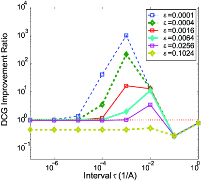
Figure 7: (color online) Effect of systematic over-rotation errors in the DCG improvement ratio for $Q=R_{\pi/4}^{(1)}$ as a function of gating interval $\tau$. In both cases, the control error strength is parametrized by $\varepsilon\in[0,1]$, and we have set $A=1$, $\Gamma=0$.

VI Extension to faulty controls and systems with drift

The explicit constructions of Sec. IV for DCGs rely on a straightforward relationship between the intended gate $Q$ and the EPG associated with it. This is enabled by assumptions (a1) and (a2) in Sec. II.1: we have focused on $H_{SB}$ (causing decoherence) as the sole source of (decoherence) errors, and the gating mechanism neither employed nor was corrupted by drift terms in $H_{S}$. In reality, as mentioned, classical errors due to control imperfections and additional quantum errors due to non-trivial unitary evolution are likely to be present to a lesser or greater extent. As also mentioned, robust control methods have been devised for separately tackling these errors, whose impact may be deleterious even if isolation from the environment is good hence decoherence is not a primary concern. In a way, composite pulse techniques for systematic control errors Alway and Jones (2007); Brown et al. (2004); Cummins and Jones (2000); Khaneja et al. (2005) may themselves be considered as a classical dynamical error correction strategy: they are perturbative in nature; they assume no quantitative knowledge of the value of errors and are constructed from building blocks of primitive pulses. Likewise, strongly modulating and gradient-ascent pulse engineering techniques in NMR Fortunato et al. (2002); Boulant et al. (2003); Luy et al. (2005) share with DQEC the basic idea of suppressing unwanted (but known) coupled-spin dynamics through coherent time-averaging, numerical search being explicitly invoked to synthesize an optimal modulation.

The above considerations prompt the need for exploring DQEC under more relaxed control assumptions than (a1) and (a2). In particular, a natural question is whether it is possible to produce hybrid dynamical error correction strategies to simultaneously counter different types of classical and quantum errors, over which a different degree of knowdlege may be available to begin with. While this question is too broad in scope to be answered in full here, and might be best treated in conjunction with numerical optimization approaches, we nonetheless illustrate the flexibility of analytic DQEC methods by providing three specific examples of DCG DCG constructions beyond (a1) and (a2).

VI.1 Towards hybrid composite-pulse/
DCG constructions

A large class of systematic control errors may be naturally modeled at the Hamiltonian level. That is, recalling Eq. (8), we may assume that the nominal gating Hamiltonian $H_{\text{gate}}(t)$ during the interval $[t_{1},t_{2}]$ is modified as

$$H^{\prime}_{\text{gate}}(t)=H_{\text{gate}}(t)+H_{S,g}+\varepsilon H_{\text{\text{dev}}}(t),$$ (40)

where $H_{\text{dev}}(t)$ is (typically gate-dependent) Hamiltonian whose functional form is known, and $\varepsilon$ is (possibly unknown) real number such that

$$\left\|U_{\text{gate}}(t_{2},t_{1})-T_{+}\Big{[}\!\exp\Big{(}\!\!\!-i\!\int_{t_{1}}^{t_{2}}\!\!\!H_{\text{ctrl}}(s)ds\Big{)}\Big{]}\right\|\ll 1.$$

The systematic nature of the error is implicit in the existence of a functional dependence between $H^{\prime}_{\text{gate}}(t)$ and $H_{\text{dev}}(t)$ as a mapping between time-dependent functions. For physically relevant error models, this mapping is often specified in terms of simple relationships between the control and the error Hamiltonian – e.g., for a single qubit, application of an $X$ gating Hamiltonian may induce a ‘parallel’ (in-axis) deviation Hamiltonian also proportional to $X$, or a ‘perpendicular’ (off-axis) deviation Hamiltonian proportional to $Y,Z$ (see also Zhang et al. (2008); Santos and Viola (2008)).

More generally, a relatively simple description of systematic control errors may be established by directly incorporating and examining their effects into the error action operator. Thus for each target gate $Q$ ideally implemented via $H_{\text{gate}}(t)$ but actually implemented via $H^{\prime}_{\text{gate}}(t)$ in the presence of the bath, to first order in the gate duration we can expand the associated total error action $\Phi$ as:

$$\Phi=\Phi_{SB}+\Phi_{\text{ctrl}},$$ (41)

where for simplicity we have assumed that no contribution arises from $H_{S}$ (or that the latter commutes with $H_{SB}$ and $\Phi_{\text{ctrl}}$ accounts for systematic control errors. The assumptions (a1)-(a2) allowed us to let $\Phi_{\text{ctrl}}=0$, and provided indirect control over $\Phi_{SB}$ through the gating interval $\tau$: For primitive gates in the absence of non-commutative drift terms, $\Phi_{SB}$ is linearly proportional to $\tau$. Such a dependence of $\Phi_{SB}$ on $\tau$ could then be explicitly utilized in the constructions of Sec. IV.2 for matching the errors in $QQ^{\prime}$ and $Q_{1/2}$.

Fixed systematic errors [cf. Eq. (39)] refer to $\Phi_{\text{ctrl}}$ terms in Eq. (41) that do not scale with $\tau$, as opposed to scaled systematic errors that scale linearly with $\tau$. Hamiltonian-control errors as described by Eq. (40) always lead to scaled systematic errors. Since the latter can be formally absorbed into $\Phi_{SB}$, in the absence of additional (drift) errors, the constructions of Sec. IV.2 may still be used to effectively reduce the effect of systematic control errors in the same way the effects of the bath are corrected. That is, arbitrary DCGs are intrinsically robust against scaled systematic errors. The EDD construction for noop on the other hand (as a special DCG), is tolerant of all, scaled and not, systematic control errors (as long as they are small), for they as can be absorbed into generator gate errors $\Phi_{F_{{}_{i}}}$ Viola and Knill (2003). The numerical results of Sec. V.2 confirm instead the expectation that generic DCG gates need not be robust under fixed systematic errors.

It is still plausible that one may use a combination of composite pulses and DCGs to actively stabilize quantum gates against both decoherence and systematic errors. The starting point is a composite pulse construction that in the absence of the environment can generate a desired gate $Q$ robustly with respect to systematic errors within a specific model. Let us assume that it is possible to modify the control inputs for this construction to obtain the gates $Q_{1/2}$ and $Q^{{}^{\prime}}$ defined in Sec. IV, such that $Q_{1/2}$ and $Q^{\prime}$ constructed in this way are also composite pulse robust against the same control errors. Then clearly the DCG construction that employs $Q$, $Q^{\prime}$, $Q_{1/2}$, along with the generator gates $F_{i}$, will correct (to first order) the systematic errors and the errors due to the bath. This, however, necessarily involves longer and more complex sequences of primitive control Hamiltonians.

VI.2 Qubits in rotating frames

An important class of systems with drift are qubits which are defined in terms of two (non-degenerate) internal energy levels and are addressed using resonance techniques. This is, for instance, the typical setting in both liquid- and solid- state NMR QIP devices Cor . In this case, the internal open-system Hamiltonian $H_{\text{int}}$ includes ‘chemical-shift’ terms of the form $H_{S}=\sum_{i}\Omega_{i}Z_{i}$, which are employed for single-qubit manipulations by moving to a frame which rotates with the applied carrier frequency $\Omega_{c}$ and by tuning on-resonance with the target spin(s). The rotating frame transformation has the effect of introducing an explicit time-dependence in system (hence system-bath) operators, according to

$${\cal O}\mapsto\tilde{\cal O}(t,t_{0})=\exp(-it\Omega_{c}\sum_{i}Z_{i})\,{\cal O}\,\exp(it\Omega_{c}\sum_{i}Z_{i}),$$

where we have assumed that $t_{0}=0$. Thus, even neglecting contributions to $\tilde{H}_{S}$ from off-resonance qubits, both the interaction with the environment and therefore the error Hamiltonian are transformed, in general, into carrier-modulated Hamiltonians $\tilde{H}_{SB}(t,0)$ and $\tilde{H}_{e}(t,0)$, respectively. This causes most of the constructions in the current paper (including EDD) to be not immediately applicable to compensate the rotating-frame error associated with a gate, because this error will generally depend on the time at which the gate is applied. Still, thanks to the known periodicity of the time dependence of the error actions, it is possible to synchronize the duration of the applied primitive gates with the rotating frame period $2\pi/\Omega$, in such a way that the relationships between the errors assumed in EDD and DCG constructions are stroboscopically preserved.

Furthermore, in practice the frequency $\Omega_{c}$ may be much higher than typical inverse gate durations. This results in rapidly oscillating terms in the rotating franes that are effectively canceled [when Eq. (11) is used with $\tilde{H}_{e}(t)$]. If $H_{e}$ consists of arbitrary single-qubit error terms [Eq. (5)], then in the limit of high carrier frequencies, the effective error model for the open-system dynamics in the rotating frame approaches the pure dephasing error model, since any terms proportional to $X^{(i)}$ and $Y^{(i)}$ in the error action will be averaged to zero, whereas any terms proportional to $Z^{(i)}$ will be time-independent. This has two implications: On the one hand, single-qubit drift terms in $H_{S}$ are of no concern for DQEC in the important case where the physical error model is dephasing to begin with; on the other hand, if arbitrary decoherence is the appropriate model in the physical frame, DCG constructions for pure dephasing are directly applicable in the rotating frame in the limit of large $\Omega_{c}$.

VI.3 Always-on qubit-qubit interactions

Aside from single-qubit drift terms as discussed above, another common type of drift contributions may arise from always-on two-qubit couplings in $H_{S}$. In NMR QIP, for instance, the latter can either be ‘$J$-coupling’ Ising-like Hamiltonians for weakly interacting spin systems, or Heisenberg-like Hamiltonians in the strong-coupling regimes. Within our present approach, the main complication that a non-switchable component $H_{S,g}$ in the gating Hamiltonian for $Q$ introduces towards constructing a DCG version is in establishing the existence of the required $Q_{1/2}$ and $Q^{\prime}$ gates, since $H_{S,g}$ effectively imposes a limit on the range of achievable control inputs. Specifically, the constructions of Sec. IV depend on generating propagators $U^{\prime}_{\text{gate}}(t,0)$ and $U^{\prime\prime}_{\text{gate}}(t,0)$, and it is not immediately clear whether universal control over the system $S$ suffices for realizing such propagators (as a one-parameter family of time-dependent operators as opposed to just end-point unitaries), even in an approximate sense. Nonetheless, we see no fundamental obstacle to treating such cases through strong modulation of the system’s dynamics and numerical optimization. To further support our optimism, we show here how analytical DCG constructions remain feasible upon careful consideration of the relevant constraints on a case-by-case basis.

Consider a system of $n$ Heisenberg-coupled qubits in a nearest-neighbor configuration:

$$H_{S}=\lambda\sum_{i=1}^{n-1}\mathbf{S}^{(i)}\cdot\mathbf{S}^{(i+1)},$$ (42)

where $\lambda\in{\mathbb{R}}$ is a fixed coupling strength. Given $H_{S}$ in Eq. (42), universal control over $S$ can be gained by assuming access to a switchable control Hamiltonians of the following form:

$$H_{\text{ctrl}}(t)=\sum_{i}[h_{X}^{(i)}(t)X^{(i)}+h_{Y}^{(i)}(t)Y^{(i)}],$$ (43)

where as usual the control inputs $h_{\alpha}^{(i)}(t)$ are subject to the power and bandwidth constraints (c1)-(c2). We assume the bath to interact with $S$ according to the arbitrary linear decoherence model: $H_{SB}\in\Omega^{\{1\}}_{e}$. Our goal is to provide a (first-order) DCG construction for the following gates: $\exp[-i\theta S_{\alpha}^{(k)}]$, where $\alpha=X,Y$, and $\exp[-i\theta\mathbf{S}^{(k)}\cdot\mathbf{S}^{(k+1)}]$, such that the resulting EPG scales with $\tau_{\min}^{2}$. Our methodology here will be somewhat different from Sec. IV, in the sense that primitive gates are not directly used as the basis of DCG constructions.

We first make the following general observation: Suppose that the gating propagator and the error Hamiltonian for a control block in the interval $[0,T]$ can be respectively written as $U_{\text{gate}}(0,t)=U_{g,1}(t)U_{g,2}(t)$ and $H_{e}=H_{e,1}+H_{e,2}$, in such a way that

$$[U_{g,1}(t),U_{g,2}(t^{\prime})]=0,$$ (44)

$$[U_{g,1}(t),H_{e,2}]=[U_{g,2}(t),H_{e,1}]=0.$$ (45)

Using the above equations and the tools of Sec. II.3, we can write the error associated with this block up to the first order as $\Phi^{[1]}=\Phi_{1}^{[1]}+\Phi_{2}^{[1]}$, where

$$\Phi_{1}^{[1]} = \int_{0}^{T}U_{g,1}(t)^{\dagger}H_{e,1}U_{g,1}(t)dt,$$ (46)

$$\Phi_{2}^{[1]} = \int_{0}^{T}U_{g,2}(t)^{\dagger}H_{e,2}U_{g,2}(t)dt.$$ (47)

As it turns out, generating a two-qubit gate on a target qubit pairs, $\exp[-i\theta\mathbf{S}^{(k)}\cdot\mathbf{S}^{(k+1)}]$, is the most non-trivial step. In this case, we clearly have $H_{S,g}=\mathbf{S}^{(k)}\cdot\mathbf{S}^{(k+1)}$ and $H_{S}-H_{S,g}=H_{S,e}$. Basically, our strategy is to first devise a scheme for dynamically correcting all error terms affecting any qubit other than $k$ and $k+1$, and next to superpose a scheme that remove any additional error term while steering the target qubits according to $H_{S,g}$. For the first step, consider the DD group $\mathcal{G}_{\text{NN}}=\mathbb{Z}_{2}\otimes\mathbb{Z}_{2}\otimes\mathbb{Z}_{2}\otimes\mathbb{Z}_{2}$, designated to decouple the subspace of bilinear qubit terms

$$\Omega_{k}^{\{2\}}=\{S_{\alpha}^{(i)}S_{\beta}^{(i+1)}\otimes B_{\alpha}^{(i)}\},$$

where $i=1,\cdots,k-1,k+1,\cdots,n-1$, $B_{\alpha}^{(i)}\in\mathcal{B}(H_{B})$ and $S_{\beta}^{(i+1)}$ may include the identity operator $I^{(i+1)}$. $\mathcal{G}_{\text{NN}}$ has 16 elements, and 4 generators which we choose to represent in ${\cal H}_{S}$ via

$$\{F_{1,j}\}=\{X^{\text{odd}}X^{\text{ev}},X^{\text{odd}}Y^{\text{ev}},\;\;\;Y^{\text{odd}}X^{\text{ev}},Y^{\text{odd}}Y^{\text{ev}}\},$$ (48)

where

$$S_{\alpha}^{\text{odd}}=\prod_{j\in E_{k}}S_{\alpha}^{(j)},\;\;S_{\alpha}^{\text{ev}}=\prod_{j\in O_{k}}S_{\alpha}^{(j)},$$

$$E_{k} = \{j\,|\,j\text{ even};0<j\leq n;j\neq k,k+1\},$$

$$O_{k} = \{j\,|\,j\text{odd};0<j\leq n;j\neq k,k+1\}.$$

Consider the EDD sequence based on $\{F_{i,1}\}$, and let $H_{g,1}(t)$ be the gating Hamiltonian associated with it over the interval $[0,T_{\text{two}}]=[0,16\times 4\tau]$, assuming as usual that each generator is implemented over an interval of length $\tau$. Note that $H_{g,1}(t)$ can be generated through appropriate combinations of the switchable inputs in Eq. (43).

In the second step, we construct the entangling gate $\exp[-64i\tau\lambda\mathbf{S}^{(k)}\cdot\mathbf{S}^{(k+1)}]$ by applying another control Hamiltonian $H_{g,2}(t)$ in parallel with $H_{g,1}(t)$. $H_{g,2}(t)$ implements a sequence very similar to the EDD sequence for the group $\mathcal{G}_{\text{LD}}=\mathbb{Z}_{2}\otimes\mathbb{Z}_{2}$ designated to cancel errors in the subspace

$$\Omega_{LD,k}=\{S_{\alpha}^{(i)}\otimes B_{\alpha}^{(i)}\,|\,i=k,k+1\}.$$

However, while the original EDD sequence would employ the generators $X^{(k)}X^{(k+1)}$ and $Y^{(k)}Y^{(k+1)}$ (or a similar combination), we now replace the two original bilinear generators with

$$F_{1,2} = X^{(k)}X^{(k+1)}\exp[-16i\tau\lambda\mathbf{S}^{(k)}\cdot\mathbf{S}^{(k+1)}],$$

$$F_{2,2} = Y^{(k)}Y^{(k+1)}\exp[-16i\tau\lambda\mathbf{S}^{(k)}\cdot\mathbf{S}^{(k+1)}].$$

The modified EDD sequence can be implemented through the available control Hamiltonians via a collective gating Hamiltonian of the form

$$H_{g,2}(t)=H_{l}^{(k)},\;\;\text{ for }t\in[8(l-1)\tau,8l\tau],$$

with

$$H_{l}^{(k)}=\begin{cases}\begin{subarray}{c}\frac{\pi}{16\tau}[X^{(k)}+X^{(k+1)}]+H_{S,g}\end{subarray},\,&l=1,3,6,8,\\ \begin{subarray}{c}\frac{\pi}{16\tau}[Y^{(k)}+Y^{(k+1)}]+H_{S,g}\end{subarray},\,&l=2,4,5,7.\end{cases}$$ (49)

Notice that the system gating Hamiltonian, explicitly included in $H_{g,2}(t)$, commutes with the single qubit terms acting on $k$ and $k+1$ in Eq. (49). Let

$$U_{g,l}(t) = T_{+}\Big{[}\exp\Big{(}-i\int_{0}^{64\tau}\!H_{\text{g},l}(s)ds\Big{)}\Big{]},$$

$$H_{e,1} = \lambda\sum_{\begin{subarray}{c}i=1\\ i\neq k\end{subarray}}^{n}\mathbf{S}^{(i)}\cdot\mathbf{S}^{(i+1)}+\sum_{\alpha}\!\sum_{\begin{subarray}{c}i=1\\ i\neq k,k+1\end{subarray}}^{n}\!\!S_{\alpha}^{(i)}\otimes B_{\alpha}^{(i)}+H_{B},$$

$$H_{e,2} = \sum_{\alpha}\sum_{i=k}^{k+1}S_{\alpha}^{(i)}\otimes B_{\alpha}^{(i)}.$$

We may thus readily verify Eqs. (44)-(45). Also notice that the total gating Hamiltonian commutes with $\mathbf{S}^{(k)}\cdot\mathbf{S}^{(k+1)}$. Thus, the overall action of the control block defined via $H_{g,1}(t)+H_{g,2}(t)$ is given by $U_{g,1}(64\tau)U_{g,2}(64\tau)=\exp[-64i\tau\lambda\mathbf{S}^{(k)}\cdot\mathbf{S}^{(k+1)}]$, and we can derive the error associated with the whole sequence (of length $T_{\text{two}}=64\tau$) by invoking Eqs. (46)- (47):

$$\Phi_{1}^{[1]} = \int_{0}^{T}\!U_{g,1}(t)^{\dagger}H_{e,1}U_{g,1}(t)dt=\sum_{l}\Phi_{1,l}^{[1]},$$

$$\Phi_{2}^{[1]} = \int_{0}^{T}\!U_{g,2}(t)^{\dagger}H_{e,2}U_{g,2}(t)dt=\sum_{l}\Phi_{2,l}^{[1]},$$

where $\Phi_{1,l}^{[1]}$ and $\Phi_{2,l}^{[1]}$ respectively denote the errors due to $H_{e,1}$ and $H_{e,2}$, associated with interval $[(l-1)\tau,l\tau]$. By (EDD) construction

$$\Phi_{1}^{[1]}=\sum_{j=1}^{4}\Pi_{\mathcal{\mathcal{G}_{\text{NN}}}}(\Phi_{F_{1,j}}).$$

One can verify directly [similar to Sec. IV.3.1] that using $H_{g,1}(t)$ results in an error $\Phi_{F_{1,j}}$ associated with each generator $F_{1,j}$ that belongs to $\Omega_{k}^{\{2\}}$, and thus we have $\Phi_{1}^{[1]}=0\text{ mod}B$. Similarly, one may also verify that the error $\Phi_{2,l}^{[1]}$ belongs to $\Omega_{\text{LD},k}$. We may then use Eq. (15) and the fact that the commutator between $\lambda\mathbf{S}^{(k)}\cdot\mathbf{S}^{(k+1)}$ and $\sum_{i=k}^{k+1}S_{\alpha}^{(i)}\otimes B_{\alpha}^{(i)}$ can be ignored up to $O[\tau^{2}\max(\|B_{\alpha}^{i)}\|)\lambda]$ to write

$$\Phi_{2}^{[1]}=\sum_{j=1}^{2}\Pi_{\mathcal{G}_{\text{LD}}}(\Phi_{F_{2,j}}),$$

therefore $\Phi_{2}^{[1]}=0\text{ mod}B$. The total error associated with this sequence is thus 0 modulo pure bath terms and terms that scale with $\tau^{2}$, as desired.

Implementing a DCG version of a single-qubit rotation $Q$ on a selected target qubit $k$ is conceptually more straightforward. In this case, $H_{S}\equiv H_{S,e}$ thus $H_{e}=H_{SB}+H_{S}$, and the DCG construction of Sec. IV can be reproduced with ease by letting the relevant error subspace cover all nearest-neighbor bi-linear interactions of the form

$$\Omega^{\{2\}}_{e}=\{S_{\alpha}^{(i)}S_{\beta}^{(i+1)}\otimes B_{\alpha}^{(i)}\},$$

where $i=1,\cdots,n-1$ and $B_{\alpha}^{(i)}\in\mathcal{B}(H_{B})$. The space $\Omega^{\{2\}}_{e}$ can be decoupled by the group $\mathcal{G}_{\text{NN}}$ with a representation similar to Eq. (48), except that now the sets $E_{k}$ and $O_{k}$ are chosen as

$$E_{k} = \{j\,|\,j\text{ even};0<j\leq n\},$$

$$O_{k} = \{j\,|\,j\text{ odd};0<j\leq n\}.$$

Similarly, we may generate $Q$, $Q^{\prime}$, and $Q_{1/2}$ by simply switching the appropriate single-qubit Hamiltonian on the $k$-th qubit. One may verify that the error associated with each control segment belongs to $\Omega^{\{2\}}_{e}$. The final DCG construction will thus contain $64$ segments for EDD and $32$ segments for $Q_{1/2}$ and $QQ^{\prime}$, for a total duration of $T_{\text{single}}=96\tau$.

It is worth noting that, in a way, the larger number of control segments emerging from the above analysis as compared to driftless scenarios may be simply regarded as an analytically generated ‘digitized’ pulse shape, with a basic time-step determined by $\tau_{\text{min}}$. Attention must be paid, however, to the fact that longer control sequences might potentially invalidate the (sufficient) convergence assumptions implicit in DCG constructions. This highlights the importance of finding an optimal DCG construction for a given control scenario. In this sense, the constructions of this section should be considered as a proof-of-concept as opposed to optimal results that might best be tailored to specific control scenarios and will likely involve a combination of analytical and numerically optimized control designs.

VII Conclusion and outlook

We have provided the mathematical and control-theoretic framework for DCGs as introduced in Ref. Khodjasteh and Viola, 2009a, and further explored their range of applicability. Besides examining in full detail the analytical construction of decoherence-protected gates in the prototypical scenario of arbitrary single-qubit errors, a physically motivated setting involving spin-bath decoherence has been characterized through exact numerical simulation. This has both confirmed the expected performance of DCGs in a wide parameter regime and yielded insight into the interplay of different open-system and control features. Additional challenges arising in the synthesis of DGCs under realistic control assumptions involving drifts and control errors have been laid out, and proof-of-concept solutions constructed in specific representative situations.

Our present analysis naturally points to several directions for further investigation. First, our focus here has been on DCG constructions that cancel errors only up to the first order in Magnus expansion. In principle, it is possible to go beyond the first order DCG constructions and produce even more efficient DQEC protocols Khodjasteh and Viola (2009b). While this will unavoidably involve a higher level of sophistication in the resulting control modulation and/or the computational effort involved in numerical search processes, a clear understanding of relevant complexity properties is needed. Making contact with the concept of ‘quantum control landspace’ as recently proposed for the generation of unitary transformations in closed quantum systems Hsieh and Rabitz (2008) might prove especially insightful.

Second, we only considered a limited set of permissible control Hamiltonians for DCG constructions. A general analysis of what we referred to as the ‘gate permissibility problem’ for a given open quantum systems is, as mentioned, still lacking. This generalization appears even more interesting by observing that the set of permissible controls can be directly related to the specific representation of the DD group used in the DCG construction. In fact, the apparent freedom in the choice of DD representation independently motivates the existence of DQEC proposals for the same tasks as DCGs that do not rely upon DD explicitly. Numerical optimization is, in this sense, a compelling option to consider for investigating more general DQEC constructions.

Lastly, different options exist for incorporating DQEC protocols into actual QIP architectures. While we have stressed the potential usefulness of DCGs directly at the physical level, DCG constructions could potentially be envisioned on top of a logical encoding, for instance to reduce EPGs in silicon double-quantum-dot logical qubits as considered in Levy et al. . Once an algorithm is specified, whether at the physical or logical level, one may further consider whether to produce the DCG version of each circuit gate, and obtain an error-suppressed algorithm accordingly; or whether instead to dynamically correct the whole algorithm viewed as a complex unitary transformation. While a thorough understanding of such design issues is fundamental for real-world applications, optimal solutions will ultimately depend on various details and constraints in place and, as such, are most effectively addressed in specific contexts. It is our hope that this work will prompt further interest and investigation in DQEC approaches from the QIP implementation community.

Appendix A Numerical methods

The simulations described in Sec. V.2 were performed (in Mathematica) using direct exact exponentiation for obtaining the propagators describing the system-plus-bath dynamics in the presence of control. Arbitrary precision matrices turned out to be necessary for the following reasons: (i) Small errors correspond to toggling-frame error propagators that are close to identity, thus it is essential that any numerical error be much smaller than the physical effect being probed. (ii) Each matrix multiplication effectively reduces the precision of the calculation by a fixed amount which depends on the dimension of the matrices used. We were limited to consider a relatively small system/bath and use matrices of very high precision [60 digits or higher] throughout the computations.

References

- DiVincenzo (2000) D. P. DiVincenzo, Fortschr. Phys. 48, 771 (2000).
- Nielsen and Chuang (2000) M. A. Nielsen and I. L. Chuang, Quantum Computation and Quantum Information (Cambridge University Press, Cambridge, UK, 2000).
- Kitaev (1997) A. Y. Kitaev, Russ. Math. Surv. 52, 1191 (1997).
- Preskill (1998) J. Preskill, Proc. R. Soc. London A 454, 385 (1998).
- Knill et al. (1998) E. Knill, R. Laflamme, and W. H. Zurek, Science 279, 342 (1998).
- Steane (2003) A. M. Steane, Phys. Rev. A 68, 042322 (2003).
- Knill (2005) E. Knill, Nature 434, 39 (2005).
- Haeberlen (1976) U. Haeberlen, High Resolution NMR in Solids: Selective Averaging (Academic Press, New York, 1976).
- (9) D. G. Cory et al., Fortschr. Phys. 48, 875 (2000).
- (10) C. Ryan, C. Negrevergne, M. Laforest, E. Knill, and R. Laflamme, eprint arXiv:0803.1982.
- Viola and Lloyd (1998) L. Viola and S. Lloyd, Phys. Rev. A 58, 2733 (1998).
- Viola et al. (1999a) L. Viola, E. Knill, and S. Lloyd, Phys. Rev. Lett. 82, 2417 (1999a).
- Viola and Knill (2005) L. Viola and E. Knill, Phys. Rev. Lett. 94, 060502 (2005).
- Santos and Viola (2006) L. F. Santos and L. Viola, Phys. Rev. Lett. 97, 150501 (2006).
- (15) K. Khodjasteh and D. A. Lidar, Phys. Rev. Lett. 95, 180501 (2005); Phys. Rev. A 75, 062310, (2007).
- (16) G. S. Uhrig, Phys. Rev. Lett. 98, 100504 (2007); ibid. 102, 120502 (2009).
- (17) A. J. Berglund, eprint arXiv:quant-ph/0010001.
- Fraval et al. (2005) E. Fraval, M. J. Sellars, and J. J. Longdell, Phys. Rev. Lett. 95, 030506 (2005).
- Morton et al. (2006) J. Morton, A. Tyryshkin, A. Ardavan, S. Benjamin, K. Porfyrakis, S. Lyon, and G. Briggs, Nature Phys. 2, 40 (2006).
- Morton et al. (2008) J. Morton, A. Tyryshkin, R. Brown, S. Shankar, B. Lovett, A. Ardavan, T. Schenkel, E. Haller, J. Ager, and S. A. Lyon, Nature 455, 1085 (2008).
- (21) S. Damodarakurup, M. Lucamarini, G. D. Giuseppe, D. Vitali, and P. Tombesi, Phys. Rev. Lett. 103, 040502 (2009).
- (22) M. J. Biercuk, H. Uys, A. P. VanDevender, N. Shiga, W. M. Itano, and J. J. Bollinger, eprint arXiv:0812.5095; eprint arXiv:0902.2957.
- Khodjasteh and Viola (2009a) K. Khodjasteh and L. Viola, Phys. Rev. Lett. 102, 080501 (2009a).
- Levitt (1986) M. H. Levitt, Progr. NMR Spectrosc. 18, 61 (1986).
- Alway and Jones (2007) W. G. Alway and J. A. Jones, J. Magn. Res. 189, 114 (2007).
- Brown et al. (2004) K. R. Brown, A. W. Harrow, and I. L. Chuang, Phys. Rev. A 70, 052318 (2004).
- Khaneja et al. (2005) N. Khaneja, T. Reiss, C. Kehlet, T. Schulte-Herbrüggen, and S. J. Glaser, J. Magn. Res. 172, 296 (2005).
- Hill (2007) C. D. Hill, Phys. Rev. Lett. 98, 180501 (2007).
- Fortunato et al. (2002) E. M. Fortunato, M. A. Pravia, N. Boulant, G. Teklemariam, T. F. Havel, and D. G. Cory, J. Chem. Phys. 116, 7599 (2002).
- Boulant et al. (2003) N. Boulant, K. Edmonds, J. Yang, M. A. Pravia, and D. G. Cory, Phys. Rev. A 68, 032305 (2003).
- Luy et al. (2005) B. Luy, K. Kozbar, T. E. Skinner, N. Khaneja, and S. J. Glaser, J. Magn. Res. 179, 176 (2005).
- Pasini et al. (2008) S. Pasini, T. Fischer, P. Karbach, and G. S. Uhrig, Phys. Rev. A 77, 032315 (2008).
- Pryadko and Quiroz (2008) L. P. Pryadko and G. Quiroz, Phys. Rev. A 77, 012330 (2008).
- Sengupta and Pryadko (2005) P. Sengupta and L. P. Pryadko, Phys. Rev. Lett. 95, 037202 (2005).
- Viola and Knill (2003) L. Viola and E. Knill, Phys. Rev. Lett. 90, 037901 (2003).
- Terhal and Burkard (2005) B. M. Terhal and G. Burkard, Phys. Rev. A 71, 012336 (2005).
- Khodjasteh and Viola (2009b) K. Khodjasteh, D. A. Lidar, and L. Viola, eprint arXiv:0908.1526.
- Zurek (2003) W. H. Zurek, Rev. Mod. Phys. 75, 715 (2003).
- Breuer and Petruccione (2002) H.-P. Breuer and F. Petruccione, The Theory of Open Quantum Systems (Oxford University Press, Oxford, 2002).
- Knill et al. (2000) E. Knill, R. Laflamme, and L. Viola, Phys. Rev. Lett. 84, 2525 (2000).
- Bhatia (1997) R. Bhatia, Matrix Analysis, no. 169 in Graduate Texts in Mathematics (Springer-Verlag, New York, 1997).
- Lidar et al. (2008) D. A. Lidar, P. Zanardi, and K. Khodjasteh, Phys. Rev. A 78, 012308 (2008).
- Khodjasteh and Lidar (2008) K. Khodjasteh and D. A. Lidar, Phys. Rev. A 78, 012355 (2008).
- D’Alessandro (2007) D. D’Alessandro, Introduction to Quantum Control and Dynamics (CRC Press, Boca Raton, 2007).
- Khodjasteh and Lidar (2005) K. Khodjasteh and D. A. Lidar, Phys. Rev. Lett. 95, 180501 (2005).
- Uhrig (2007) G. S. Uhrig, Phys. Rev. Lett. 98, 100504 (2007).
- (47) H. Uys, M. J. Biercuk, and J. J. Bollinger, arXiv:0904.0036.
- Khodjasteh and Lidar (2007) K. Khodjasteh and D. A. Lidar, Phys. Rev. A 75, 062310 (2007).
- Santos and Viola (2008) L. F. Santos and L. Viola, New J. Phys. 10, 083009 (2008).
- Rötteler and Wocjan (2006) M. Rötteler and P. Wocjan, IEEE Trans. Inf. Theory 52, 4171 (2006).
- Viola et al. (2000) L. Viola, E. Knill, and S. Lloyd, Phys. Rev. Lett. 85, 3520 (2000).
- Viola (2002) L. Viola, Phys. Rev. A 66, 012307 (2002).
- Lidar (2008) D. A. Lidar, Phys. Rev. Lett. 100, 160506 (2008).
- Not (a) Within the radius of convergence, the Magnus expansion is absolutely convergent. This fact can be used to cap the sum of the higher order terms, see e.g. Khodjasteh and Lidar (2007).
- Aliferis and Preskill (2008) P. Aliferis and J. Preskill, Phys. Rev. A 78, 052331 (2008).
- Not (b) The so-called Uhrig DD is an example where the algebraic simplicity of the dephasing model is exploited to obtain an efficient DQEC protocol Uhrig (2007).
- Viola (2004) L. Viola, J. Mod. Opt. 51, 2357 (2004).
- (58) Interestingly, a close-in-spirit implementation has been recently reported for dynamical suppression of collisional decoherence in cold trapped atoms, see Y. Sagi, I. Almog and N. Davidson, eprint arXiv:0905.0286.
- Viola et al. (1999b) L. Viola, S. Lloyd, and E. Knill, Phys. Rev. Lett. 83, 4888 (1999b).
- Loss and DiVincenzo (1998) D. Loss and D. P. DiVincenzo, Phys. Rev. A 57, 120 (1998).
- Hanson et al. (2007) R. Hanson, L. P. Kouwenhoven, J. R. Petta, S. Tarucha, and L. M. K. Vandersypen, Rev. Mod. Phys. 79, 1217 (2007).
- Zhang et al. (2007a) W. Zhang, N. P. Konstantinidis, K. A. Al-Hassanieh, and V. V. Dobrovitski, J. Phys.: Cond. Matter 19, 083202 (2007a).
- Not (c) Identical DCG constructions would be valid if the Heisenberg interaction is replaced by any two-qubit Hamiltonian commuting with (e.g., the Ising interaction).
- Not (d) In principle, the unit step function could be replaced by any function such that and . Even different gates need not be based on the same profile . The essential requirement, however, is that the control profiles are flexible enough to allow the constructions of and in Sec. IV.2.
- Zhang et al. (2007b) W. Zhang, V. V. Dobrovitski, L. F. Santos, L. Viola, and B. N. Harmon, Phys. Rev. B 75, 201302(R) (2007b).
- Zhang et al. (2007c) W. Zhang, V. V. Dobrovitski, L. F. Santos, L. Viola, and B. N. Harmon, J. Mod. Opt. 54, 2629 (2007c).
- Zhang et al. (2008) W. Zhang, N. P. Konstantinidis, V. V. Dobrovitski, B. N. Harmon, L. F. Santos, and L. Viola, Phys. Rev. B 77, 125336 (2008).
- (68) Realization-to-realization fluctuations in the improvement ratio and corresponding fidelities have been found to be more or less pronounced depending on parameter regime. In particular, the variations are largest for and large (yielding e.g. up to a relative variance over different samples), whereas the effect of seems far less important. These fluctuations do not in any case qualitatively alter the main observed features.
- Cummins and Jones (2000) H. K. Cummins and J. A. Jones, New J. Phys. 2, 6.1 (2000).
- Hsieh and Rabitz (2008) M. Hsieh and H. Rabitz, Phys. Rev. A 77, 042306 (2008).
- (71) J. E. Levy, A. Ganti, C. A. Phillips, B. R. Hamlet, A. J. Landahl, T. M. Gurrieri, R. D. Carr, and M. S. Carroll, eprint arXiv:0904.0003.