Can the particle mass spectrum be explained within the Standard Model?

Abstract

A modified version of PQCD considered in previous works is investigated here in the case of retaining only the quark condensate. The Green functions generating functional is expressed in a form in which Dirac’s delta functions are now absent from the free propagators. The new expansion implements the dimensional transmutation effect through a single interaction vertex in addition to the standard ones in mass less QCD. The new vertex suggest a way for constructing an alternative to the SM in which the mass and CKM matrices could be generated by the instability of masslesss QCD under the production of the top quark and other fermions condensates, in a kind of generalized Nambu Jona Lasinio mechanism. The results of a two loop evaluation of the vacuum energy indicate that the quark condensate is dynamically generated. However, the energy as a function of the condensate parameter is again unbounded from below in this approximation. Assuming the existence of a minimum of the vacuum energy at the experimental value of the top quark mass $m_{q}=173$ $GeV$, we evaluate the two particle propagator in the quark anti-quark channel in zero order in the coupling and a ladder approximation in the condensate vertex. Adopting the notion from the former $top$ quark models, in which the Higgs field corresponds to the quark condensate, the results suggests that the Higgs particle could be represented by a meson which might appear at energies around two times the top quark mass.

I Introduction

The origin of the singular structure of the particle mass spectrum is one of the central questions in  Particle Physics.   Although the Standard Model (SM) furnishes a remarkable description of the physical experience, the issue about better understanding the  mass hierarchy has been always present in the research activity nambu ; fritzsch ; coleman ; bardeen ; miransky ; minkowski ; clague . In particular, this circumstance is reflected in the unsatisfying large  number of parameters which should be fixed in the SM to describe the observed masses. Therefore, the search of  new approaches to consider this problem is an important theme of study nowadays.

A development of  an alternative perturbation expansion for QCD,  including the presence of quark and gluon condensates in the free vacuum state generating the Wick expansion, has been considered in previous works mpla ; prd ; epjc ; epjc1 ; jhep ; epjc2 ; hoyer ; hoyer1 ; hoyer2 ; epjc19 .  A basic issue motivating the study is the question about what could be the final strength of a  dynamically generated  quark condensate in mass less QCD, in which the free vacuum is strongly degenerated  and the underlying forces are the strongest ones in Nature coleman .  This point motivated the search for modifications of the Wick expansion in this theory starting from free vacuum states including zero momentum gluon and quark condensates, in order to afterwards adiabatically connect the interaction prd ; jhep ; epjc .  A similar modification of the free vacuum leading to the perturbative expansion, but filling real particles states up to a Fermi level was before considered by P. Hoyer hoyer .   The modified expansion following from Ref. mpla ; prd ; epjc ; epjc1 ; jhep ; epjc2 ; epjc19 has also close connections with other independent approaches in the literature. Those consider modified free particle vacua and propagators in generating the perturbative expansion in order to take into account condensate effects celenza ; roberts ; pavel . Finally, we expect that in the future the analysis can show links with well established non perturbative theories considering condensation effects such as the Sum Rules approach and the Fukuda gluon condensation studies shifman ; fukuda . We would like to remark that the modified expansion being investigated could perhaps represent a theoretical foundation for the ”superconductivity systems ” like properties of the particle mass spectrum underlined in Refs. nambu ; fritzsch ; fritzsch1 ; bardeen . This possibility is signaled by the fact that the fermion condensate generation closely resembles the similar effect in the usual BCS theory. This fact is a natural outcome since the free vacua employed to generate the expansion have the same BCS like ”squeezed” state structureprd .  In Ref.mpla ; prd ; epjc ; epjc1 ; jhep ; epjc2 ; epjc19 some indications about the possible dynamic generation of quark and gluon condensates had been obtained. Nevertheless, this correction to the vacuum energy turned out to be unbounded from below as a function of the quark condensate.   In this work  we  restrict the discussion to the simpler case in which there is only one quark condensate present in the system. It is natural to firstly consider this  situation, since the aim is to investigate the possibility that  large dynamic quark condensates and masses could define a kind of $top$ quark model  as an effective action for mass less QCD.  In this  case, the Green’ functions generating functional $Z$ of the system obtained in Ref.epjc19 , is here transformed to a more helpful representation. In this form $Z$ is expressed as the same functional integral associated  to mass less  QCD, in which all the effects of the condensates are now embodied in only one special  vertex  having two quark and two gluon legs. This representation allows to systematize the  diagrammatic expansion of the problem. In particular it permits to  implement the dimensional transmutation effect.    The obtained path integral formula  can be expected to be also helpful in developing perturbative schemes in superconductivity theory.  This formula is perhaps the central result of the present work, because it indicates a technical path through which the approach being considered, could help to evidence that  an strong instability of massless QCD under the generation of fermion condensates, can be the explanation of the whole particle mass hierarchy (including quark and leptons) in  a sort of  generalized  Nambu-Jona Lasinio SSB mechanism nambu ; fritzsch ; bardeen ; miransky . Specifically, the structure of the vertex indicates ways for its generalization  which seem able to describe the quark mass and CKM matrices as coming from the first terms in an effective action.

The application of the expansion is nambu ; fritzsch ; coleman ; bardeen ; miransky ; minkowski ; clague considered in this work, by calculating the leading logarithm of the condensate dependence of a two loop approximation considered for the effective potential. The results repeat the indication of the dynamic generation of the quark condensate obtained in previous works epjc2 ; epjc19 , but again, the potential results to be unbounded from below.  However, in the present case, the obtained leading logarithm behavior reinforces the instability for large values of the quark condensate. This outcome rises the need of performing new evaluations that could determine a minimum. The attainment of stability in the next three loop approximation is  feasible, since  squared logarithms of the condensate terms should appear, that upon showing the appropriate sign can produce a global minimum of the potential.  The evaluation of the squared logarithm corrections at the three loop level is expected to be considered elsewhere.

The work also present an evaluation of the two particle propagator in a $t\overline{t}$ channel in zero order in the coupling and a ladder approximation in the condensate vertex. The singularities of the result are then analyzed by assuming the existence of a minimum of the vacuum energy at the experimental value of the top quark mass $m_{q}=173$ GeV.  In this case, after also adopting the notion from the former $top$ quark models, in which the Higgs field corresponds to the quark condensate, the results suggest that the Higgs particle should be considered as a $t\overline{t}$ meson which could appear at energies around to two times the $top$ quark mass.  The  mass of this meson bound state is expected to be estimated after adding the gluon exchange contribution to the kernel of the Bethe-Salpeter equation, to the here evaluated only condensate dependent kernel.

The work proceeds as follows.  In Section II the function integral formula for the states showing a quark condensate  is derived.   Section III is devoted to evaluate two correction for the vacuum energy as  function of the condensate parameter.  The Section IV  then consider the evaluation of the two particle Green function in ladder approximation in terms of the new condensate vertex and the zero order in the coupling. Finally the results are reviewed in the Summary.

II A functional integral for quark condensate states

In this section we will  present a simpler representation of the generating functional of the modified massless QCD  in which a fermion condensate is introduced to define the initial vacuum state employed to generate the Wick expansion epjc19 .  The unrenormalized form of the functional will be considered. In this case all the condensate parameters are absent from the vertices. The expression for the complete generating functional introduced in Ref. epjc19 as restricted to a vanishing gluon condensate can be written in the form

$$Z[j,\xi,\xi^{\ast},\eta,\overline{\eta}] =\exp[i\int dx\int\mathcal{L}_{1}(\frac{\delta}{i\delta j^{a,\mu}},\frac{\delta}{i\delta\xi^{\ast}}\frac{\delta}{-i\delta\xi}\frac{\delta}{i\delta\overline{\eta}}\frac{\delta}{-i\delta\eta})]\times$$ (1)

$$Z^{(0)}[j,\xi,\xi^{\ast},\eta,\overline{\eta}],$$

$$Z^{(0)}[j,\xi,\xi^{\ast},\eta,\overline{\eta}] =Z^{G}[j]Z^{FP}[\xi,\xi^{\ast}]Z^{F}[\eta,\overline{\eta}],$$ (2)

$$\mathcal{L}_{1}(A_{\mu},\chi,\chi,\psi,\overline{\psi}) =-\frac{g}{2}f^{abc}(\partial_{\mu}A_{\nu}-\partial_{\nu}A_{\mu})A^{b\mu}A^{c\nu}-g^{2}f^{abe}f^{cdec}A_{\mu}^{a}A_{\nu}^{b}A^{c\mu}A^{d\nu},-$$

$$-gf^{abc}\partial^{\mu}(\chi^{a\ast})\chi^{b}A_{\mu}^{c}+g\overline{\psi}T^{a}\gamma^{\mu}\psi A_{\mu}^{a},$$ (3)

where the free generating functionals associated  the gluon, ghosts and quark fields take the expressions

$$Z^{G}[j] =\exp[\frac{i}{2}\int dx\text{ }dy\text{ }j^{a\mu}(x)D_{\mu\nu}^{ab}(x-y)\text{ }j^{b\nu}(x)],$$

$$Z^{FP}[\xi,\xi^{\ast}] =\exp[i\int dx\text{ }dy\text{ }\xi^{a\ast}(x)D(x-y)\text{ }\xi^{a}(x)],$$

$$Z^{F}[\eta,\overline{\eta}] =\exp[i\int dx\text{ }dy\text{ }\overline{\eta}(x)S^{C}(x-y)\eta(y)].$$

The exponential operator $\exp[i\int dx\int\mathcal{L}_{1}(\frac{\delta}{i\delta j^{a,\mu}},\frac{\delta}{i\delta\xi^{\ast}}\frac{\delta}{-i\delta\xi}\frac{\delta}{i\delta\overline{\eta}}\frac{\delta}{-i\delta\eta})]$ will be denominated in what follows as the $vertex$ $part$. By the assumption of vanishing  gluon condensate, the gluon and ghost propagators are the usual Feynman ones and the quark propagator includes the condensate dependent part as

$$S^{C}(x-y)=\int\frac{dk}{(2\pi)^{D}}(\frac{1}{-p_{\mu}\gamma^{\mu}}-i\text{ }C\text{ }\delta^{D}(p))\exp(-i\text{ }p.x).$$

Let us repeat below, for this simpler case of  only having the quark condensate, the procedure employed in epjc19 for linearizing in the sources the exponential arguments in the generating functional. The free quark generating functional can be rewritten  in the form

$$Z^{F}[\eta,\overline{\eta}]=\exp[i\int dxdy\text{ }\overline{\eta}(x)S(x-y)\eta(y)]\times\exp[\int dx\text{ }\overline{\eta}(x)\frac{C}{(2\pi)^{D}}\int dy\text{ }\eta(y)],$$

and the quadratic in the sources argument of the exponential can be represented as a linear one after expressing the exponential as the result of the gaussian integral

$$\exp[\int dx\text{ }\overline{\eta}(x)\frac{C}{(2\pi)^{D}}\int dy\text{ }\eta(y)] =\int\mathcal{D}\overline{\chi}\mathcal{D}\chi\exp[-\overline{\chi}\chi+$$

$$+i{\Large(}\int dx\text{ }\overline{\eta}(x)\frac{1}{i}(\frac{C}{(2\pi)^{D}})^{\frac{1}{2}}\chi+\overline{\chi}\frac{1}{i}(\frac{C}{(2\pi)^{D}})^{\frac{1}{2}}\int dy\text{ }\eta(y){\Large)].}$$

As a consequence of the  implemented linearity in the sources, the condensate parameter $C$ dependent terms can be shifted to the left of the $vertex$ $part$ functional operator in equation (1) by employing the following general relation

$$\mathcal{F[}\frac{\delta}{i\delta\overline{\eta}},\frac{\delta}{-i\delta\eta}]\exp[i{\Large(}\int dx\text{ }\overline{\eta}(x)\frac{1}{i}(\frac{C}{(2\pi)^{D}})^{\frac{1}{2}}\chi+\overline{\chi}\frac{1}{i}(\frac{C}{(2\pi)^{D}})^{\frac{1}{2}}\int dy\text{ }\eta(y){\Large)]}$$

$$=\exp[i{\Large(}\int dx\text{ }\overline{\eta}(x)\frac{1}{i}(\frac{C}{(2\pi)^{D}})^{\frac{1}{2}}\chi+\overline{\chi}\frac{1}{i}(\frac{C}{(2\pi)^{D}})^{\frac{1}{2}}\int dy\text{ }\eta(y){\Large)]\times}$$

$$\mathcal{F[}\frac{\delta}{i\delta\overline{\eta}}+\frac{1}{i}(\frac{C}{(2\pi)^{D}})^{\frac{1}{2}}\chi,\frac{\delta}{-i\delta\eta}+\overline{\chi}\frac{1}{i}(\frac{C}{(2\pi)^{D}})^{\frac{1}{2}}].$$

Then, after again representing as functional integrals, the free generating functionals associated to the gluons, ghosts and quarks, by also acting on them  with the new terms appeared in the $vertex$ $part$ after the above described commutations, a modified free theory generating functional can be written in the following way epjc19

$$Z^{(0,C)}[j,\eta,\overline{\eta},\xi,\overline{\xi}|C_{q}] =\frac{1}{\mathcal{N}}\int\int\int d\overline{\chi}d\chi\mathcal{D}[A,\overline{\Psi},\Psi,\overline{c},c]\exp[i\text{ }S^{(0)}[A,\overline{\Psi},\Psi,\overline{c},c,\overline{\chi},\chi]]$$

$$=\frac{1}{\mathcal{N}}\int\int d\overline{\chi}d\chi\exp[-\overline{\chi}_{u}^{i}\chi_{u}^{i}]\int\mathcal{D}[A,\overline{\Psi},\Psi,\overline{c},c]\times$$

$$\times\exp[-i\int\frac{dk}{(2\pi)^{D}}[\frac{1}{2}A_{\mu}^{a}(-k)(k^{2}g^{\mu\nu}-(1-\frac{1}{\alpha})k_{\mu}k_{\nu})A_{\nu}^{a}(k)+$$

$$i\int\frac{dk}{(2\pi)^{D}}\overline{c}^{a}(-k)k^{2}c^{a}(k)+$$

$$+i\int\frac{dk}{(2\pi)^{D}}\overline{\Psi}^{i}(-k)\text{ }\gamma_{\mu}k^{\mu}\,\Psi^{i}(k)\text{ }+$$

$$+i\int\frac{dk}{(2\pi)^{D}i}\overline{\Psi}^{i,u}(-k)\text{ }g(\frac{C_{q}}{(2\pi)^{D}})^{\frac{1}{2}}\gamma_{\mu}^{u\text{ }v}T_{a}^{ij}\,\chi^{j,v}\text{ }A^{\mu,a}(k)+$$

$$+i\int\frac{dk}{(2\pi)^{D}i}A^{\mu,a}(-k)\overline{\chi}^{i,u}\text{ }g(\frac{C_{q}}{(2\pi)^{D}})^{\frac{1}{2}}\text{ }\gamma_{\mu}^{u\text{ }v}T_{a}^{ij}\,\Psi^{j,v}(k)+$$ (4)

$$+i\int\frac{dk}{(2\pi)^{D}}(j_{\mu}(-k)A^{\mu}(k)+\overline{\eta}(-k)\Psi(k)+\overline{\Psi}(k)\eta(-k)+$$

$$\overline{\xi}(-k)c(k)+\overline{c}(-k)\xi(k))].$$

It corresponds to the general relation obtained epjc19  after taking a vanishing gluon condensate parameter. The complete generating functional is obtained by acting on it with the usual $vertex$ $part$ functional operator. It should be noted that the above expression has been written in its Minkowski space form,  since in this work we will adopt the same conventions and notations as in Ref. muta . In the formula $A$, $\Psi$  and $c$  are the gluon, quark and ghost fields and $\overline{\chi},\chi$ are the space independent auxiliary parameters which were introduced in Ref. epjc19 in order to represent the quadratic forms in the sources as linear ones. The mentioned in the Introduction simplification of the perturbative expansion,  comes from noticing that in  expression (4)  the integral over the auxiliary fields is a Gaussian one.  Therefore, it can be explicitly integrated by finding the values of the auxiliary fields which solve the Lagrange equations following from the action laying in the argument of the exponential integrand.  These equations of motion take the simple forms

$$\frac{\delta S^{(0)}[A,\overline{\Psi},\Psi,\overline{c},c,\overline{\chi},\chi]}{\delta\overline{\chi}_{u}^{i}} =-\chi_{u}^{i}+i\int\frac{dk}{(2\pi)^{D}i}A^{\mu,a}(-k)g(\frac{C_{q}}{(2\pi)^{D}})^{\frac{1}{2}}\text{ }\gamma_{\mu}^{u\text{ }v}T_{a}^{ij}\,\Psi^{j,v}(k)=0,$$ (5)

$$\frac{\delta S^{(0)}[A,\overline{\Psi},\Psi,\overline{c},c,\overline{\chi},\chi]}{\delta\chi_{u}^{i}} =\overline{\chi}_{u}^{i}-i\int\frac{dk}{(2\pi)^{D}i}\overline{\Psi}^{j,v}(-k)\text{ }g(\frac{C_{q}}{(2\pi)^{D}})^{\frac{1}{2}}\gamma_{\mu}^{vu\text{ }}T_{a}^{ji}\,\text{ }A^{\mu,a}(k)=0.$$ (6)

Henceforth, after substituting the expressions for the  auxiliary fields  in   equation (4), the free generating functional can be written as follows

$$Z^{(0)} =\frac{1}{\mathcal{N}}\int\mathcal{D}[A,\overline{\Psi},\Psi,\overline{c},c]\exp[iS^{(0)}[A,\overline{\Psi},\Psi,\overline{c},c]+i\text{ }S^{(C_{q})}[A,\overline{\Psi},\Psi]],$$ (7)

$$\text{ }S^{(0)}[A,\overline{\Psi},\Psi,\overline{c},c] =\left.S^{(0)}[A,\overline{\Psi},\Psi,\overline{c},c,\overline{\chi},\chi]\right|_{\overline{\chi},\chi=0},$$ (8)

where the two terms linear in the auxiliary fields have been substituted by the action $S^{(C_{q})}$ , having the expression

$$S^{C_{q}}[A,\overline{\Psi},\Psi] =\frac{g^{2}C_{q}}{i(2\pi)^{D}}\int\frac{dk}{(2\pi)^{D}}\overline{\Psi}^{i,u}(-k)\gamma_{\mu}^{uv}T_{a}^{ij}A^{\mu,a}(k)\times$$

$$\int\frac{dk^{\prime}}{(2\pi)^{D}}A^{\mu^{\prime},a^{\prime}}(-k^{\prime})\gamma_{\mu^{\prime}}^{vu^{\prime}}T_{a}^{ji^{\prime}}\Psi^{i^{\prime}u^{\prime}}(k^{\prime})$$

$$=\frac{g^{2}C_{q}}{i(2\pi)^{D}}\int\int dxdx^{\prime}\overline{\Psi}^{i,u}(x)\gamma_{\mu}^{uv}T_{a}^{ij}A^{\mu,a}(x)A^{\mu^{\prime},a^{\prime}}(x^{\prime})\gamma_{\mu^{\prime}}^{vu^{\prime}}T_{a^{\prime}}^{ji^{\prime}}\Psi^{i^{\prime}u^{\prime}}(x^{\prime})$$

$$=\frac{g^{2}C_{q}}{i(2\pi)^{D}}\int\int dxdx^{\prime}\overline{\Psi}(x)\not{A}(x)\not{A}(x^{\prime})\Psi^{{}^{\prime}}(x^{\prime}).$$ (9)

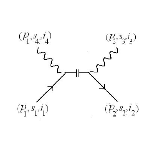
Figure 1: The diagram shows the structure of the new vertex which must be added to the Feynman diagram rules of mass less QCD to describe the modified Wick expansion of the theory in presence of a quark condensate in the free vacuum.

In the last line of the equation, $\overline{\Psi}^{i,u}(x)$ and $\Psi^{i^{\prime}u^{\prime}}$ are understood as vectors with composite indices formed by the color and spinor ones and $\not{A}$ should correspondingly be interpreted as a matrix with such kind of indices also. This term defines a new interaction vertex  which convey all the information about the fermion condensate.    By adding now the action terms associated to the other usual interaction vertices of mass less QCD, the full expression for the generating functional of the modified PQCD can be  written in the form

$$Z[j,\eta,\overline{\eta},\xi,\overline{\xi}|C_{q}]=\frac{1}{\mathcal{N}}\int\mathcal{D}[A,\overline{\Psi},\Psi,\overline{c},c]\exp[i\text{ }S[A,\overline{\Psi},\Psi,\overline{c},c]+i\text{ }S^{C_{q}}[A,\overline{\Psi},\Psi]],$$ (10)

in which now $S$ is the full action defining mass less QCD muta :

$$S =\int dx(\mathcal{L}_{0}\mathcal{+L}_{1}\mathcal{)},$$

$$\mathcal{L}_{0} =\mathcal{L}^{g}+\mathcal{L}^{gh}+\mathcal{L}^{q},$$

$$\mathcal{L}^{g} =-\frac{1}{4}(\partial_{\mu}A_{\nu}^{a}-\partial_{\nu}A_{\mu}^{a})(\partial^{\mu}A^{a,\nu}-\partial^{\nu}A^{a,\mu})-\frac{1}{2\alpha}(\partial_{\mu}A^{\mu,a})(\partial^{\nu}A_{\nu}^{a}),$$

$$\mathcal{L}^{gh} =(\partial^{\mu}\chi^{\ast a})\partial_{\mu}\chi^{a},$$ (11)

$$\mathcal{L}^{q} =\overline{\Psi}(i\gamma^{\mu}\partial_{\mu})\Psi,$$

$$\mathcal{L}_{1} =-\frac{g}{2}f^{abc}(\partial_{\mu}A_{\nu}^{a}-\partial_{\nu}A_{\mu}^{a})A^{b,\mu}A^{c,\nu}-g^{2}f^{abe}f^{cde}A_{\mu}^{a}A_{\nu}^{b}A^{c,\mu}A^{d,\nu}-$$

$$-gf^{abc}(\partial^{\mu}\chi^{\ast a})\chi^{b}A_{\mu}^{c}+g\overline{\Psi}T^{a}\gamma^{\mu}\Psi A_{\mu}^{a}.$$

At this point we would like to comment about the possibility for a natural way of generalizing the form of the new vertex to introduce the interactions between quarks and leptons of different flavors.  The proposal has the form

$$S^{C}[A,\overline{\Psi},\Psi]=\sum\limits_{f_{1},f_{2}}^{\sigma_{1},\sigma_{2}}\frac{C_{f_{1}f_{2}}^{\sigma_{1}\sigma_{2}}}{i(2\pi)^{D}}\int\int dxdx^{\prime}\overline{\Psi}_{f_{1},\sigma_{1}}(x)\not{A}(x)\not{A}(x^{\prime})\Psi_{f_{2},\sigma_{2}}(x^{\prime}),$$ (12)

where $f_{1},f_{2}$ are quark flavor indices and $\sigma_{1},\sigma_{2}$ are weak interactions $SU(2)$ ones. Note that this structure could be even more generalized to include the six lepton flavors. The  discussion in Ref. jhep , by example,  directly suggests that the Feynman expansion  generated have the chance of allowing to  phenomenologically reproduce the quark mass and CKM matrices of the SM. This possibility in conjunction with the definition of a ground state in which the condensate stabilizes,  can give also add support to the  alternative expansion being investigated.  These issues are expected to be considered elsewhere.

III Two loop leading logarithm correction to the Effective Potential

Let us in this section consider the vacuum energy (the negative of the Effective Potential) as a function of the  condensate parameter. The general motivation is to investigate  the possibility for obtaining a  minimal energy vacuum state around which the systems stabilizes. This stabilization, then, can open the way for the interest to investigate the physical predictions of the perturbation expansion around this stable state. In particular the most ambitious expectation is the possibility for generating the  physics of the SM from a generalized version of the scheme after including the rest of the fields needed to such an objective.

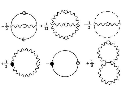
Figure 2: The two loop correction to the Effective Action considered in this work. It corresponds to the sum of the same two loop diagrams of mass less QCD, but in which the free mass less quark and gluon propagators were substituted by dressed counterparts.

The specific approximation to be taken for the Effective Potential will be the following one. We will consider the same summation of two loop graphs of mass less QCD, but substituting the  mass less free quark and gluon propagators by $dressed$ expressions. These ones will be propagators associated to self-energies taken in their lowest non vanishing order in terms of the condensate dependent vertex defined in (9) and Fig. 1.  The two loop contributions are shown in Fig. 2. In this picture the above mentioned quark and gluon propagators are indicated by the usual wavy and straight lines respectively, but adding open circles their mid points. The large black dots denote the counterterm vertices of QCD appearing in the considered two loop approximation. Further below the appearing  gluon and quark lines without circles will mean the usual free propagators  of mass less QCD in the conventions of Ref. muta  The $dressed$ quark propagator  will  be the one generated by the infinite ladder of insertions of the one loop self energy illustrated in Fig 3a) .  For  the gluons, the fact that the one loop self-energy (polarization operator) contribution vanishes, requires to consider the two loop gluon self energy terms which Feynman diagrams are shown in Fig 3b).  At this point it could be useful to recall that the evaluations considered in the paper were done by following the notations and conventions of  Ref.  muta . As above noted, the  Feynman graph and its analytic expression of the new vertex to be added to the standard ones in Ref. muta are defined in Fig. 1 and Eq. (9).

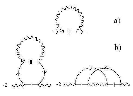
Figure 3: Figure a) shows the one loop quark self-energy diagram employed for constructing the dressed quark propagator in the ladder approximation. Figure b) illustrates the two loop self-energy correction employed to define the gluon dressed propagator also in the ladder approximation. A two loop correction was required because the one loop one vanishes. For this exploration, these corrections were chosen to only depend on the new condensate vertex.

The  gluon and quark self-energy evaluations in Fig. 3 need only for the calculation of some spinor and color traces, since the loop integrals  are canceled in both cases by the Dirac’s Delta functions appearing in the condensate dependent vertex. The results for them has the expressions

$$\Sigma_{i,j}^{u,v}(p) =-S\frac{\delta^{ij}\delta^{uv}}{p^{2}},$$ (13)

$$S =-\frac{g^{2}C_{q}}{(2\pi)^{D}}\frac{D(N^{2}-2)}{2N},$$ (14)

$$\Pi_{\mu\nu}^{ab}(p) =-\frac{\delta^{ab}}{(p^{2})^{2}}{\large(}a\text{ }(g_{\mu\nu}-\frac{p_{\mu}p_{\nu}}{p^{2}})+(a+b)\frac{p_{\mu}p_{\nu}}{p^{2}}{\large)},$$ (15)

$$a =S^{2}\frac{8N(DN^{2}+4-2D)}{D^{2}(N^{2}-1)^{2}},\text{ \ }b=S^{2}\frac{16N(D-2)}{D^{2}(N^{2}-1)^{2}},$$ (16)

where $D=4-2\epsilon$ is the space dimension in the dimensional regularization scheme and $N=3$ defines the $SU(3)$ group of interest here.

When the gauge $\alpha=1$ is chosen, as it will done in this work, the summations of the  geometric series representing all the ladder self-energy insertions leads for the quark propagator the expression

$$G_{i_{1}i_{2}}^{u_{1}u_{2}}(p) =\delta^{i_{1}i_{2}}{\Large(}\frac{1}{-p_{\mu}\gamma^{\mu}+\frac{S}{p^{2}}}{\Large)}^{u_{1}u_{2}}$$

$$=-\frac{\delta^{i_{1}i_{2}}}{p^{2}-\frac{S^{2}}{(p^{2})^{2}}}{\Large(}p_{\mu}\gamma^{\mu}+\frac{S}{p^{2}}{\Large)}^{u_{1}u_{2}},$$ (17)

$$S =-m_{q}^{3},$$ (18)

the quantity $m_{q}$ defines the only pole laying in the positive real axis of the propagator as a function of $\ p^{2}$. It will named in what follows as the  $quark$ $mass$. As it was discussed in Ref. epjc19 the  parameters of  perturbative expansion may be chosen to be  $g$ and $m_{q}$ .

In the case of the gluon propagator, after the summation of the geometric series associated to the sum of arbitrary insertions of the gluon self-energy illustrated in Fig. 3b), the $dressed$ gluon propagator can be written in the form

$$D_{\mu\nu}^{ab}(p) =D_{\mu\nu}^{(0)ab}(p)+D_{\mu\nu}^{(1)ab}(p)+D_{\mu\nu}^{(2)ab}(p),$$ (19)

$$D_{\mu\nu}^{(0)ab}(p) =\frac{\delta^{ab}g_{\mu\nu}}{p^{2}},$$ (20)

$$D_{\mu\nu}^{(1)ab}(p) =-\frac{a\delta^{ab}g_{\mu\nu}}{p^{2}((p^{2})^{3}+a)},$$ (21)

$$D_{\mu\nu}^{(2)ab}(p) =-\frac{b\delta^{ab}p^{2}p_{\mu}p_{\nu}}{((p^{2})^{3}+a)((p^{2})^{3}+(a+b))},$$ (22)

in which $D_{\mu\nu}^{(0)ab}$ is the free propagator and $D_{\mu\nu}^{(1)ab}(p)$ and $D_{\mu\nu}^{(2)ab}(p)$ the condensate dependent contributions which vanish if $C_{q}=0.$

Now, it can be observed that after removing the dimensional regularization, any Feynman graphs contributing to the vacuum energy of the theory will have an analytic expression of the form $m_{q}^{4}F(\log(\frac{m_{q}}{\mu})).$   In particular for the two loop expression being considered, the function $F$  is expected, at first sight to be a second order polynomial in $\log(\frac{m_{q}}{\mu})$ .    However, the enhanced convergence properties  introduced by the high dimension of the parameter $S$ allows to reduce the dependence to a linear one. To see this property, let us consider both, the gluon and the quark, propagators as decomposed in their free propagator parts  plus a contribution dependent on the condensate. After this, let us also decompose any of the two loop graphs in the superposition shown in Fig. 2, in the set of topologically identical graphs, obtained by expanding the product of all the internal propagators defining them. Let us note now the  fact that, normally  each divergent loop integration adds  a pole in to the considered two loop integrals. Then, it can be seen that thanks to the high  dimension (of value equal to $3$) of the constant $S,$ it follows that the only term in which a second order pole in $\epsilon$ can arise, is the one in which the condensate dependent parts of the propagators are not appearing. That is, in the graphs of the original mass less QCD.  Thus, there is no condensate dependent terms showing a second order pole. But, the squared logarithm $(\log(\frac{m_{q}}{\mu}))^{2}$ can only arise from such terms. Thus there are not $(\log(\frac{m_{q}}{\mu}))^{2}$  dependent terms in the considered  two loop diagrams. This rule explains why they were no logarithmic terms in the one loop approximation jhep ; epjc2 .  That is, the appearance of any condensate dependent component of the propagator in the considered set of expanded graph makes convergent one of the two loop integrals and the remaining one can at most produce a linear term in $\log(\frac{m_{q}}{\mu}).$  Further, the presence of two condensate dependent components of the propagators in two independent loops, leads to the convergence of the graph, which in these cases shows a simple $m_{q}^{4}$ dependence after removing the dimensional regularization   Thus, the leading logarithmic correction in the considered situation is linear in $\log(\frac{m}{\mu}).$

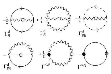
Figure 4: The diagram shows the only the divergent terms which arise after expanding the product of all the dressed quark and gluon propagators in the two diagrams of Fig. 2, when they are expressed as the sum of the free propagator plus the condensate dependent part.

The above mentioned properties permit to conclude that the only graphs in the above described expansion,  which may contribute to the leading logarithm correction are the one shown in Fig 4. Let us describe in what follows the evaluation of the contribution of each of such diagrams to the logarithmic correction.

The diagram $\Gamma_{q}^{d}$ corresponds to a line of a condensate dependent gluon propagator connected to the external vertices of the quark loop contribution $\Pi_{q}^{\mu\nu},$ to the total one loop gluon polarization operator $\Pi^{\mu\nu}$ of usual mass less QCD.  The expression for $\Pi_{q}^{\mu\nu}$can be explicitly evaluated following the conventions in Ref. muta , and $\Gamma_{q}^{d}$  takes the form

$$\Gamma_{q}^{d} =\frac{1}{2}\int\frac{dq^{D}}{(2\pi)^{D}i}D_{\mu\nu}^{(1)ab}(q)\Pi_{q}^{ba\mu\nu}(q)$$ (23)

$$=\frac{1}{2}\text{ }a\mu^{4-D}\text{ }g^{2}(N^{2}-1)(D-2)\int\frac{dq^{D}}{(2\pi)^{D}i}\frac{J_{1}(-q^{2},\epsilon)}{(q^{2})^{3}+a}$$

$$J_{1}(-q^{2},\epsilon) =\frac{1}{(4\pi)^{\frac{D}{2}}}(-q^{2})^{\frac{D}{2}-2}\times\frac{\Gamma(2-\frac{D}{2})\Gamma^{2}(\frac{D}{2}-1)}{\Gamma(D-2)},$$ (24)

$$\Pi_{q}^{ba\mu\nu}(q) =-\frac{g^{2}}{2}\delta^{ab}\int\frac{dq^{D}}{(2\pi)^{D}i}tr_{s}[\gamma^{\mu}G^{(0)}(p+q)\gamma^{\nu}G^{(0)}(p)].$$ (25)

The term $\Gamma_{q}^{d}$  is associated to a line of  a condensate dependent gluon propagator attached to the ends of the gluon loop $\Pi_{g}^{\mu\nu}$contribution to the one loop polarization operator $\Pi^{\mu\nu}$ . This quantity also can be directly evaluated to write for this term

$$\Gamma_{g}^{d} =\frac{1}{2}\int\frac{dq^{D}}{(2\pi)^{D}i}(D_{\mu\nu}^{{}^{(1)}ab}(q)+D_{\mu\nu}^{(2)ab}(q))\Pi_{g}^{ba\mu\nu}(q)$$

$$=-\frac{a\text{ }\mu^{4-D}g^{2}}{8(D-1)}N(N^{2}-1)\int\frac{dq^{D}}{(2\pi)^{D}i}\frac{J_{1}(-q^{2},\epsilon)g^{\mu\nu}}{q2((q^{2})^{3}+a)}\times$$

$$((6D-5)q^{2}g_{\mu\nu}+(6D-7)q_{\mu}q_{\nu})+$$

$$\frac{1}{2}\int\frac{dq^{D}}{(2\pi)^{D}i}D_{\mu\nu}^{(2)ab}(q)\Pi_{g}^{ba\mu\nu}(q),$$ (26)

$$\Pi_{g}^{ba\mu\nu}(q) =\frac{1}{2}\int\frac{dk^{D}}{(2\pi)^{D}i}(-ig)f^{acd}V_{\mu\lambda\rho}(-q,k+q,-k)\frac{g^{\lambda\kappa}}{(q+k)^{2}}\times$$ (27)

$$\frac{g^{\rho\sigma}}{k^{2}}(-i)f^{bdc}V_{\nu\sigma\kappa}(q,k,-k-q),$$

where the function $V_{\nu\sigma\kappa}$ defines the three legs gluon vertex as in Ref. muta .

Similarly, the term $\Gamma_{gh}^{d}$, is associated to the ghost loop contribution to $\Pi^{\mu\nu}$, can be evaluated  in the form

$$\Gamma_{gh}^{d} =\frac{1}{2}\int\frac{dq^{D}}{(2\pi)^{D}i}(D_{\mu\nu}^{(1)ab}(q)+D_{\mu\nu}^{(2)ab}(q))\Pi_{gh}^{ba\mu\nu}(q)$$

$$=\frac{a\text{ }\mu^{4-D}g^{2}}{8(D-1)}N(N^{2}-1)\int\frac{dq^{D}}{(2\pi)^{D}i}\frac{J_{1}(-q^{2},\epsilon)\text{ \ }g_{\mu\nu}}{q^{2}((q^{2})^{3}+a)}\times$$

$$((2-D)q^{\mu}q^{\nu}-q^{2}g^{\mu\nu})+\frac{1}{2}\int\frac{dq^{D}}{(2\pi)^{D}i}D_{\mu\nu}^{(2)ab}(q)\Pi_{gh}^{ba\mu\nu}(q),$$ (28)

$$\Pi_{gh}^{aa^{\prime}\mu\nu}(q) =-\int\frac{dq^{D}}{(2\pi)^{D}i}(-g^{2})\frac{p(p+q)}{p^{2}(p+q)^{2}}f^{abc}f^{a^{\prime}cb}.$$ (29)

Note that the part associated to the pure longitudinal condensate dependent propagator$\ D_{\mu\nu}^{(2)ab}$ in Eqs. (26) and (28) cancels after adding the terms $\Gamma_{gh}^{d}$ and $\Gamma_{g}^{d},$ thanks to the transversality condition satisfied by the sum of the gluon and ghost loops terms of the one loop self-energy $\Pi^{\mu\nu}$. This property is directly seen after adding $\Gamma_{gh}^{d}$ and $\Gamma_{g}^{d}$ which result can be written as

$$\Gamma_{g}^{d}+\Gamma_{gh}^{d} =\frac{1}{2}\int\frac{dq^{D}}{(2\pi)^{D}i}D_{\mu\nu}^{(1)ab}(q)(\Pi_{g}^{ba\mu\nu}(q)+\Pi_{gh}^{ba\mu\nu}(q))$$

$$=\frac{a\text{ }g^{2}}{8(D-1)}N(N^{2}-1)(6D-4)\int\frac{dq^{D}}{(2\pi)^{D}i}\frac{J_{1}(-q^{2},\epsilon)g^{\mu\nu}}{q^{2}((q^{2})^{3}+a)}\times$$

$$(q^{2}g_{\mu\nu}-q_{\mu}q_{\nu})$$

Then, the  transversal tensor appearing inside the integral eliminates the purely longitudinal component $D_{\mu\nu}^{(2)ab}$ when added to $D_{\mu\nu}^{(1)ab}$.

Further, the last of the diagrams not being associated to counterterms, $\Gamma_{gq}^{d},$ is related with a line of quark condensate dependent propagator connected to the external vertices of the  one loop contribution to the quark self-energy in usual mass less QCD. After evaluating the one loop quark self-energy $\Sigma_{sr}^{ij}$ , this term can be written as follows

$$\Gamma_{gq}^{d} =-\int\frac{dq^{D}}{(2\pi)^{D}i}G_{rs}^{ji}(q)\Sigma_{sr}^{ij}(q)$$

$$=-\text{ }\mu^{4-D}g^{2}(2-D)(N^{2}-1)\int\frac{dq^{D}}{(2\pi)^{D}i}\frac{(q^{2})^{3}J_{1}(-q^{2},\epsilon)}{((q^{2})^{3}+a)},$$ (30)

$$\Sigma_{sr}^{ij}(q) =\int\frac{dp^{D}}{(2\pi)^{D}i}\gamma_{\mu}^{r^{\prime}r}T_{j^{\prime}j}^{a}G^{(0)s^{\prime}r^{\prime}}(p)\frac{1}{(q-p)^{2}}g\text{ }\gamma^{\mu,ss^{\prime}}T_{ij^{\prime}}^{a}.$$ (31)

Next, let us write the expressions for the  diagrams related with the counterterms.  The values for the renormalization constants will be chosen as coinciding with the ones in QCD as evaluated in Ref.  muta .  The gluon counterterm loop will be decomposed in the two components being associated to the substractions $\Gamma_{g}^{c,g}$ and $\Gamma_{q}^{c,g}$ which makes finite the gluon and quark loops contribution to the polarization operator respectively, in standard QCD. These quantities can be written  in the form

$$\Gamma^{c,g} =\Gamma_{g}^{c,g}+\Gamma_{q}^{c,g},$$ (32)

$$\Gamma_{g}^{c,g} =\frac{a\text{ }\mu^{4-D}}{2}(D-1)(N^{2}-1)\delta Z_{3}^{g}\int\frac{dq^{D}}{(2\pi)^{D}i}\frac{1}{((q^{2})^{3}+a)},$$ (33)

$$\Gamma_{q}^{c,g} =\frac{a\text{ }\mu^{4-D}}{2}(D-1)(N^{2}-1)\delta Z_{3}^{q}\int\frac{dq^{D}}{(2\pi)^{D}i}\frac{1}{((q^{2})^{3}+a)},$$ (34)

$$Z_{3} =1+\delta^{g}Z_{3}+\delta Z_{3}^{f},$$ (35)

$$\delta Z_{3}^{g} =(\frac{g_{0}}{4\pi})^{2}\frac{1}{\epsilon}\frac{1}{2}C_{G}(\frac{10}{3}),$$ (36)

$$\delta Z_{3}^{q} =-(\frac{g_{0}}{4\pi})^{2}\frac{1}{\epsilon}\frac{4}{3}T_{R},$$ (37)

$$T_{R} =\frac{1}{2},\text{ \ \ }C_{G}=N.\text{\ }$$ (38)

In the case of the quark loop counterterm contribution in Fig. 4 , the   following expression can be obtained

$$\Gamma^{c,q} =4N(Z_{2}-1)\int\frac{dq^{D}}{(2\pi)^{D}i}\frac{(q^{2})^{3}}{((q^{2})^{3}+a)},$$ (39)

$$Z_{2} =1-(\frac{g}{4\pi})^{2}\frac{C_{F}}{\epsilon},$$ (40)

$$\text{\ \ }C_{F} =\frac{N^{2}-1}{2N}.$$ (41)

Note that the mass renormalization parameter has been taken equal to zero in a first instance to check whether the same renormalization constants of the massless QCD are able to eliminate the infinities in the  considered approximation. However, since we are  investigating the mass generation an improved selection could will be performed after better understanding the problem. These possibilities will be considered  in the extension of the work.

III.1 Leading logarithm corrections

The evaluations to be considered in this section will be done in Euclidean space and by selecting only the real part of the integrals.  That is, we will perform the substitution   $p_{0}\rightarrow i$ $p_{4}$ (with $p_{4}$  real) in the integrals an take the real part of it.   This means that we will be effectively calculating the real part of the zero temperature Thermodynamical Potential of the system. A difference between this quantity and the Effective Action in Minkowski  space could appear when it is attempted to perform a continuous deformation of the integration path, in order to implement the above mentioned simple substitution.  We will not analyze this effect in this paper, since it is related with possible instabilities of the systems showing such non vanishing differences. Those instabilities  can be expected to arise in this ”one condensate” calculation, by example, if not only  one, but few quark condensates are needed to be dynamically generated in order to arrive at the real ground state of the system.

After adding $\Gamma_{q}^{d}$   and $\Gamma_{q}^{c,g},$ the following expression, which explicitly shows the dependence on the dimension $D,$ can be written

$$\text{ \ }\Gamma_{q}^{d}+\Gamma_{q}^{c,g} =-(N^{2}-1)\int_{0}^{\infty}dq_{0}\int_{0}^{\infty}dr\frac{1}{(q^{2}+i\delta)^{3}+1}\frac{r^{D-2}}{(2\pi)^{D}i}\frac{2\pi^{D-1}}{\Gamma(\frac{D-1}{2})}\times$$

$${\Huge(}-\frac{(D-2)\Gamma(2-\frac{D}{2})\Gamma^{2}(\frac{D}{2}-1)}{2(4\pi)^{\frac{D}{2}}\Gamma(D-2)}(-q^{2})^{\frac{D}{2}-2}a^{\frac{D}{3}-\frac{2}{3}}\mu^{4\epsilon}g_{0}^{2}+$$

$$+\frac{(D-1)}{2}(\frac{g_{0}}{4\pi})^{2}\mu^{2\epsilon}a^{\frac{D}{6}}\frac{4}{3}T_{R}\frac{1}{\epsilon}{\Huge)},\text{ \ \ \ }$$

$$q^{2} =q_{0}^{2}-r^{2},\text{ }\epsilon=2-\frac{D}{2}.$$

Taking the limit $\epsilon\rightarrow 0$, the above formula allows to verify that the  usual counterterm of  mass less QCD  cancels the divergence of this Effective Action contribution. After the Wick substitution $q_{0}\rightarrow i$ $q_{4}$ (without considering the residues at the poles as described above)  the real part of the effective potential,  is given by the above expression  in which the integral is taken in the principal value sense. The explicit evaluation  gives for the contribution of this term to the leading logarithm correction, the result

$$V_{a}(m_{q}) =-\lim_{\epsilon\rightarrow 0}\operatorname{Re}[\Gamma_{q}^{d}+\Gamma_{q}^{c,g}]$$

$$=\frac{\pi}{2}(N^{2}-1)\frac{g_{0}^{2}\text{ }m_{q}^{4}}{384\text{ }6^{\frac{1}{3}}\pi^{5}}PP\int_{0}^{\infty}dx\text{ }x^{3}\frac{1}{-x^{6}+1}\times$$

$$(3\log(x^{2})+6\log(\frac{m_{q}}{\mu})-3\gamma-5+\log(\frac{3}{256\text{ }\pi^{3}}))$$

$$=\frac{g_{0}^{2}m_{q}^{4}}{1728\sqrt[3]{6}\pi^{3}}\left(\sqrt{3}\left(6\log\left(\frac{m_{q}}{\mu}\right)+\log\left(\frac{3}{256\pi^{3}}\right)+3\gamma-5\right)+4\pi\right).$$ (42)

Adding the terms $\Gamma_{g}^{d}$ and $\Gamma_{gh}^{d}$ with   their corresponding counterterm contribution $\Gamma_{g}^{c,g}$ the resulting dependence on the dimension $D$  is given by the formula

$$\Gamma_{g}^{d}+\Gamma_{gh}^{d}+\Gamma_{g}^{c,g} =-2(N^{2}-1)\int_{0}^{\infty}dq_{0}\int_{0}^{\infty}dr\text{ }\frac{r^{D-2}}{(2\pi)^{D}i}\frac{1}{(q^{2}+i\delta)^{3}+1}\frac{2\pi^{D-1}}{\Gamma(\frac{D-1}{2})}\times$$

$${\Huge(}\frac{\Gamma(2-\frac{D}{2})\Gamma^{2}(\frac{D}{2}-1)}{(4\pi^{\frac{D}{2}})\Gamma(D-2)}\frac{N\text{ }(3D-2)}{4(D-1)}(-q^{2})^{\frac{D}{2}-2}a^{\frac{D}{3}-\frac{2}{3}}\mu^{4\epsilon}g_{0}^{2}-$$

$$\frac{1}{4}(\frac{g_{0}}{4\pi})^{2}\mu^{2\epsilon}a^{\frac{D}{6}}\frac{1}{\epsilon}C_{G}\frac{10}{3}{\Huge)},\text{ \ \ \ \ }q^{2}=q_{0}^{2}-r^{2},$$

in which again, the $\epsilon\rightarrow 0$  limit shows that divergences are canceled by the original one loop counterterms of mass less QCD. As before, after the Wick substitution, for the real part of this contribution to the potential, the result  can be expressed as follows

$$V_{b}(m_{q}) =-\lim_{\epsilon->0}\operatorname{Re}[\Gamma_{g}^{d}+\Gamma_{gh}^{d}+\Gamma_{g}^{c,g}]$$

$$-\frac{\pi}{2}(N^{2}-1)\frac{g_{0}^{2}\text{ }m_{q}^{4}}{256\text{ }6^{\frac{1}{3}}\pi^{5}}PP\int_{0}^{\infty}dx\text{ }x^{3}\frac{1}{-x^{6}+1}\times$$

$$(15\log(x^{2})+30\log(\frac{m_{q}}{\mu})+15\gamma-31-40\log 2+\log(\frac{243}{\pi^{15}}))$$

$$=-\frac{g_{0}^{2}m_{q}^{4}}{1152\sqrt[3]{6}\pi^{3}}{\Large(}\sqrt{3}{\Large(}30\log\left(\frac{m_{q}}{\mu}\right)-15\log(\pi)+\log(243)$$

$$\text{ \ \ \ \ }-40\log(2)+15\gamma-31{\Large)}+20\pi{\Large).}$$ (43)

Finally, the quantities $\Gamma_{gq}^{d}$    and $\Gamma^{c,q}$ , after to be added can be expressed in the following form as explicit functions of the dimension $D$

Figure 5: The figure illustrates the dependence of the logarithmic in the condensate contribution to the effective potential. The curve indicates an instability of the system in the approximation being considered, under the generation of large condensate values.Thus, the approximation adopted is yet insufficient to detect the existence of a stable ground state to which the system would relax. However, the natural appearance of squared logarithms of the condensate in the next three loop approximation makes feasible that the stability can arise after considering three loop corrections.

$$\Gamma_{gq}^{d}+\Gamma^{c,q} =-g^{2}C_{F}N(2-D)J_{1}(1,\epsilon)\frac{2\pi^{\frac{D}{2}}}{\Gamma(\frac{D}{2})}\frac{S^{\frac{{}^{2}}{3}D-\frac{4}{3}}}{(2\pi)^{D}}\frac{\pi}{3}\sec(\frac{\pi}{6}(1-2D))+$$

$$+\frac{4C_{F}N}{\epsilon}(\frac{g_{0}}{4\pi})^{2}\frac{2\pi^{\frac{D}{2}}}{\Gamma(\frac{D}{2})}\frac{(S^{2})^{\frac{D}{6}}}{2(2\pi)^{D}}\frac{\pi}{3}\sec(\frac{\pi}{6}(1-2\epsilon)),$$

where as before, the standard counterterm is able to  cancel the divergence. Now, after performing the Wick substitution  the contribution to the potential in the limit  $\epsilon\rightarrow 0,$ takes the expression

$$V_{c}(m_{q}) =-\lim_{\epsilon->0}\operatorname{Re}(\Gamma_{gf}^{d}+\Gamma^{c,q})$$

$$=-\frac{g_{0}^{2}m_{q}^{4}}{216\pi^{3}}\left(\sqrt{3}\left(6\log(m_{q})-6\log(\mu)+\log\left(\frac{1}{64\pi^{3}}\right)+3\gamma-3\right)+\pi\right).$$ (44)

Finally, the  complete leading logarithm correction to the potential has the form

$$V(m_{q}) =V_{a}(m_{q})+V_{b}(m_{q})+V_{c}(m_{q})$$

$$\cong g_{0}^{2}\text{ }m_{q}^{4}{\large(}-C_{1}\text{ }\log(\frac{m_{q}}{\mu})+C_{2}{\large),}$$ (45)

$$C_{1} =8.5788\times 10^{-4},\text{ \ }C_{2}=1.21224\times 10^{-3}.$$

This component of the potential is plotted as a function of the $quark$ $mass$ in Fig. 5.  The picture illustrates the instability under the generation of  large quark condensate. However, the considered approximation, does not  furnishes yet  a  minimum around which the system can stabilize.

However, such a minimum can be a natural consequence in a three loop level at which ($\log(m_{q}))^{2}$  corrections should appear, whenever the net sign turns to be the appropriate one.  This  question is expected to be considered elsewhere.

IV The Higgs particle as a $t\overline{t}$ meson

In this section we will assume that the next three loop corrections will be able to produce a minimum in the potential and that this minimum can be fixed to occur at the top quark mass value $\ m_{q}=173$ $GeV$ .  Let us  discuss below an evaluation of the singularities of the $t$ and $\overline{t}$ two particle propagator $G_{\mu_{1},\mu_{2};\mu_{3},\mu_{4}}^{a_{1},a_{2};a_{3},a_{4}}(p_{1},p_{2})$ after to be contracted in its color and spinor indices at the input and output pairs of legs.  This contracted propagator corresponds to zero color and spin channel of the $t$ and $\overline{t}$ quarks. . The calculation will be considered in the ladder approximation  in the condensate dependent vertex  and the zero order in the coupling constant. The Fig.6 a) shows one general term of the geometric series defining the ladder approximation. Fig.6b) illustrates the basic diagram which  repetitive insertion permits generate the general diagram shown in Fig.6 a)

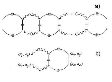
Figure 6: Figure a) shows the diagram associated to general power correction in the geometric series defining the ladder approximation to the two particle Green function. The ladder approximation refers to the zeroth order in the coupling constant approximation. That is, it only includes the condensate dependent vertex. Figure b) illustrates the repeated diagram in terms of which the geometric series was evaluated and the indices convention.

The contribution corresponds to the zeroth order in the coupling constant $g$ and a ladder approximation of the propagator in the condensate vertex.   In order to simplify the evaluation we will consider that the parameter $b$ defining the contribution $D^{(2)}(p)$ of the gluon propagator is much smaller than the parameter $a$ associated to $D^{(1)}(p)$ in the proportion $\ b/a=9/128$   Thus, the terms $D^{(2)}(p)$ will be disregarded which simplifies the discussion due to the simpler Lorentz structure of  $D^{(1)}(p)$.

The  evaluation of the repetitive block defining the ladder approximation (illustrated in Fig.6b)  leads to the  expression

$$T_{\mu_{1},\mu_{2};\mu_{3},\mu_{4}}^{a_{1},a_{2};a_{3},a_{4}}(p_{1},p_{2}) =-\frac{2(p_{1}^{2}p_{2}^{2})^{2}}{((p_{1}^{2})^{3}+a)((p_{2}^{2})^{3}+a)}(\frac{g^{2}C_{q}}{(2\pi)^{D}})^{2}Tr_{c}{\large(}T^{a_{1}}T^{a_{2}}T^{a_{4}}T^{a_{3}}{\large)}\times$$

$$Tr_{s}{\large(}\gamma_{\mu_{1}}\gamma_{\mu_{2}}G(-p_{2})\gamma^{\mu_{4}}\gamma^{\mu_{3}}G(p_{1}){\large).}$$

However, after contracting this expression under the input color indices $a_{1}$ and $a_{2}$ and the spinor ones $\mu_{1}$ and $\mu_{2}$  and employing the relations

$$Tr_{c}{\large(}T^{a_{1}}T^{a_{1}}T^{a_{4}}T^{a_{3}}{\large)} =\frac{C_{F}}{2}\delta^{a_{3}a_{4}},$$

$$Tr_{s}{\large(}\gamma_{\mu_{1}}\gamma^{\mu_{1}}G(-p_{2})\gamma^{\mu_{4}}\gamma^{\mu_{3}}G(p_{1}){\large)} =\frac{4D(-p_{1}.p_{2}+\frac{S^{2}}{p_{1}^{2}p_{2}^{2}})}{(p_{1}^{2}-\frac{S^{2}}{(p_{1}^{2})^{2}})(p_{2}^{2}-\frac{S^{2}}{(p_{2}^{2})^{2}})}g^{\mu_{3}\mu_{4}},$$

it follows that the dependence on the output color and spinor indices get the simple structure

$$g^{\mu_{1}\mu_{2}}T_{\mu_{1},\mu_{2};\mu_{3},\mu_{4}}^{a_{1},a_{1};a_{3},a_{4}}(p_{1},p_{2}) =-\frac{4DC_{F}(p_{1}^{2}p_{2}^{2})^{2}}{((p_{1}^{2})^{3}+a)((p_{2}^{2})^{3}+a)}(\frac{g^{2}C_{q}}{(2\pi)^{D}})^{2}\times$$

$$\frac{(-p_{1}.p_{2}+\frac{S^{2}}{p_{1}^{2}p_{2}^{2}})}{(p_{1}^{2}-\frac{S^{2}}{(p_{1}^{2})^{2}})(p_{2}^{2}-\frac{S^{2}}{(p_{2}^{2})^{2}})}\delta^{a_{3}a_{4}}g^{\mu_{3}\mu_{4}},$$

$$=T(p_{1},p_{2})\delta^{a_{3}a_{4}}g^{\mu_{3}\mu_{4}}.$$

Therefore, all the set of intermediate color and spinor indices in the successive blocks in the ladder expansion also contracts.  This property allows to sum the geometric series associated with the ladder approximation to write the considered Green function in the following form

$$g^{\mu_{1}\mu_{2}}G_{\mu_{1},\mu_{2};\mu_{3},\mu_{4}}^{a_{1},a_{1};a_{3},a_{3}}(p_{1},p_{2})g^{\mu_{3}\mu 4}=\frac{1}{1-T(p_{1},p_{2})}F(p_{1},p_{2})$$

where $F$ is given by the same function $T$ defined above, after being multiplied by a function of the momenta defined by the external lines of $G$. Henceforth, the singularities of this propagator in the considered approximation are defined by the zeroes of the denominator

$$0 =1-T(p_{1},p_{2})$$

$$=1+(\frac{g^{2}C_{q}}{(2\pi)^{D}})^{2}\frac{4DC_{F}(p_{1}^{2}p_{2}^{2})^{2}}{((p_{1}^{2})^{3}+a)((p_{2}^{2})^{3}+a)}\times$$

$$\frac{(-p_{1}.p_{2}+\frac{S^{2}}{p_{1}^{2}p_{2}^{2}})}{(p_{1}^{2}-\frac{S^{2}}{(p_{1}^{2})^{2}})(p_{2}^{2}-\frac{S^{2}}{(p_{2}^{2})^{2}})}.$$

This relation can be now expressed in terms of the center of mass momentum $p$ and the relative momentum $q,$ defined by

$$p =p_{1}+p_{2}$$

$$q =p_{1}-p_{2},$$

in the following form

$$1 =-\frac{S^{2}}{C_{F}}\frac{((p+q^{2})^{2}-4(p.q)^{2})^{4}}{4^{4}(\frac{(p^{2}+2p.q+q^{2})^{3}}{2^{6}}+\frac{4}{3}S^{2})(\frac{(p^{2}-2p.q+q^{2})^{3}}{2^{6}}+\frac{4}{3}S^{2})}\times$$

$$\frac{(-\frac{1}{4}(p^{2}-q^{2})+\frac{16S^{2}}{(p^{2}+q^{2})^{2}-4(p.q)^{2}})}{(\frac{(p^{2}+2p.q+q^{2})^{3}}{2^{6}}-S^{2})\frac{(p^{2}-2p.q+q^{2})^{3}}{2^{6}}-S^{2}}.$$ (46)

Now, without loss of generality, by selecting the reference frame  appropriately, these vectors can be expressed in terms of three parameters  as

$$p =(m,0,0,0),$$

$$q =(q_{0},\mathbf{q,}0,0).$$

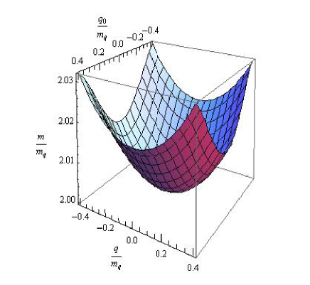
Figure 7: The figure illustrates the particle anti-particle continuous spectrum of excitations associated to the evaluated two particle Green function correction. Note that the further inclusion of the Bethe-Salpeter gluon kernel, can produce bound state below the mass threshold of the $t$ and $\overline{t}$ generation in the $top$ quark detection experiments.

One branch of solutions of the dispersion relation (46), expressed as the values of the $center$ $of$ $mass$ $energy$  $m$ as a function of the component of the relative momentum $q_{0}$ and $\mathbf{q,}$ is illustrated in Fig.  7.  The plot shows a continuous spectrum  with a mass threshold equal to twice the $top$ quark mass $m_{q}$. This results is a natural one in the here considered approximation, in which the order $g^{2}$ gluon interacting kernel has not been considered.  The obtained spectrum  also suggests that the Higgs particle in the here considered scheme, should correspond to a possibly existing short living $t\overline{t}$ bound state  appearing below the $2m_{p}=346$ $\ GeV$  mass threshold. This meson can be expected to be described by the present picture after  also introducing .the gluon kernel into the Bethe-Salpeter equation associated with the here examined two  particle Green function.

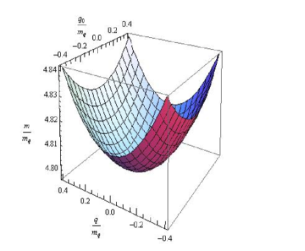
Figure 8: A second continuous spectrum branch of $t\overline{t}$ excitations following from the considered zeroth order in the coupling two points Green function. Note that it shows a threshold near $4.8m_{q}.$

The dispersion relation (46) shows another threshold for continuous excitation. It is shown in Fig. 8. The mass gap in this case is at a value $4.8$ $m_{q}$= $830.4$ $GeV$ . Thus, after including the color binding kernel an excited state of the $t\overline{t}$ meson could exists near this higher threshold.

V Summary

In this work a functional integral representation has been presented which  promises to be helpful in the study of ground states showing a quark condensate. The analysis suggests that it could be also technically useful in applications to systems  showing superconductivity. Although the discussion is only restricted to the presence of a single quark condensate, the extension to the case of the inclusion of other quark and gluon condensates seems to be feasible.   The new vertex opens possibilities for start the construction of an alternative to the SM in which the mass and CKM matrices are determined  by  the condensation of the various quarks and leptons. Thus, the results suggest that the instability of the massless QCD could be the driving force generating the hierarchical particle mass spectrum, though a kind of generalized Nambu-Jona Lasinio mechanism. The procedure is employed here to  study the possibility for the existence of a stable ground state showing a quark condensate, through a two loop evaluation  of  the vacuum energy. For this purpose, the leading logarithm dependence  on the quark condensate parameter of the two loop correction to the Effective Potential is calculated. The result indicates that the system is unstable under the generation of large values of the condensate, but a stabilization point in the dependence is not following in the considered approximation. However, the expected  to appear quadratic terms in $\log(\frac{m_{q}}{\mu})$  at the three loop level,   have the chance of determining  a minimum of the potential.   In addition, improved evaluations of the vacuum energy, not being based in the recourse of  simply substituting the mass less propagators by approximate $dressed$ ones in the usual loop expansion, can also be of help. These possibilities are expected to be considered in the extension of the work.

The expansion is also employed to evaluate the two particle  Green function associated to a color and scalar singlet channel in the ladder approximation in terms of the condensate dependent vertex. Assumed that the quark mass can be fixed to the observed value, the evaluation in this simple approximation shows a continuous spectrum of excitation  above a mass threshold equal to two times the $top$ quark mass.  Therefore, following the idea of the old  $top$ condensate models, in which the role of the Higgs is played by the $t\overline{t}$ condensate, the discussion indicates that the Higgs could correspond to a $t\overline{t}$ bound state meson which could be detected below the threshold  found in the experiments for finding the top quark.  The study of such bound states after incorporating the  gluon kernel in the Bethe-Salpeter equation is expected to be considered in extending the work.

Before ending, let us comment on two important issues both connected with the extension of the work. The first of them is related with the possibility that the mechanism under discussion can  describe the $top$ quark and $\Lambda_{QCD}$ mass scales at the same time.  This opportunity is suggested after noticing two main properties: a) The logarithmic dependence of the effective potential on the quark mass $m_{q}$  and b)  The presence of terms in the effective potential of the form   $-|a|$ $m_{q}^{4},$ reflecting the instability.  To see it, let us consider the potential in two loops (at more loops, higher powers of the logarithm will appear) as written in the form

$$V(m_{q}) =-|a|\text{ }m_{q}^{4}\text{ }+b\text{ }m_{q}^{4}\text{ }\log\frac{m_{q}}{\mu}$$

$$=|b|\text{ }m_{q}^{4}\text{ }\log(\frac{m_{q}}{\exp(\frac{|a|}{b})\mu}),$$

where it is assumed that after the exact evaluation of the finite terms (having a dependence of the form $m_{q}^{4})$, the resulting coefficient shows the negative value $-|a|$   Further assume that the extremum of the potential as a function of $m_{q}$ , is situated at the $top$ quark mass $m_{q}=173$ GeV    and also that the dimensional regularization parameter $\mu$ is approximately given by $\Lambda_{QCD}$ $\approx 0.1$ GeV.   Therefore, after finding the extremum of the potential over $m_{q}$, the ratio of the coefficients $\frac{|a|}{|b|}$ is estimated as follows

$$0 =m_{q}^{3}\text{ }(4\log(\frac{m_{q}}{\exp(\frac{|a|}{b})\mu})+1)\rightarrow\exp(\frac{|a|}{b})=\exp(\frac{1}{4})\frac{m_{q}}{\mu}$$

$$\frac{|a|}{|b|} =|\log(\exp(\frac{1}{4})\frac{m_{q}}{\mu})|\approx\log(\exp(\frac{1}{4})\frac{173\text{ GeV}}{0.1\text{ GeV}})=7.70.$$

Henceforth, since the instability created by the $QCD$ forces can be strong, it seems feasible that a not so large ratio value of $\frac{|a|}{|b|}=7.7$ could arise after evaluating the finite terms, then giving space for these two widely different scales be both predicted by the scheme.

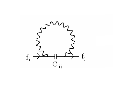
Figure 9: The figure show the effective action two legs diagrams through which the generalized theory including all sort of condensates from the start could be able to generate the Yukawa mass and CKM matrices.

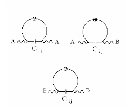
Figure 10: The figure illustrates few diagrams in the effective action of the generalized theory with two legs of weak interaction bosons, which could generate the masses of the $W$ and $Z$ particles.

The second point about we which to remark is connected with the possibility for constructing a variant of the SM model starting from the here presented discussion. This idea may directly come to the mind by noticing that the mass terms associated to the quark and leptons in a fist approximation for an effective model are associated to the graph of the form illustrated in figure 9 showing one condensate vertex with two external fermion legs and a massive gluon propagator joining the two gluon legs of the vertex. In the before proposed generalized form of the vertex the indices $f$ can correspond to quarks or leptons, a fact that lead to idea of fixing the matrix $C_{f_{1},f_{2}}$ to reproduce the Yukawa mass matrix. Note that the large mass of the gluon modified propagator should make the interaction between the input and output fermions short ranged and then the vertex effectively produce a Yukawa term. Figure 10 simply intends to show some diagrams of the considered generalized model which could generate the masses for the $W$ and $Z$ particles starting from the massless $SU(2)$ and $U(1)$ vector gauge fields of the SM model.The possibilities indicated above are in some measure supported by the fact that in the context of the usual top condensate models, it has been argued that the top anti-top condensate technically implements the role of the Higgs field.

References

• (1) Y. Nambu and G. Jona-Lasinio, Phys. Rev. 122, 345 (1961).
• (2) H. Fritzsch, Nucl. Phys. B155, 189 (1979).
• (3) S. Coleman and E. Weinberg, Phys. Rev. D7, 1888 (1973).
• (4) W. A. Bardeen, C. T. Hill and M. Lindner, Phys. Rev. D41, 1647 (1990).
• (5) V.A. Miransky, in Nagoya Spring School on Dynamical Symmetry Breaking, ed. K. Yamawaki, World Scientific (1991).
• (6) H. Fritzsch and P. Minkowski, Phys. Rep. 73, 67 (1981).
• (7) D. E. Clague and G. G. Ross, Nucl. Phys. B364, 43 (1991).
• (8) A. Cabo, S. Peñaranda and R. Martínez, Mod. Phys. Lett. A10, 2413 (1995).
• (9) M. Rigol and A. Cabo, Phys. Rev. D62, 074018 (2000).
• (10) A. Cabo and M. Rigol, Eur. Phys. J. C23, 289 (2002).
• (11) A. Cabo and M. Rigol, Eur. Phys. J. C47, 95 (2006).
• (12) A. Cabo and D. Martinez-Pedrera, Eur. Phys. J. C47, (2006).
• (13) P. Hoyer, NORDITA-2002-19 HE (2002), e-Print Archive: hep-ph/0203236 (2002).
• (14) P. Hoyer, Proceedings of the ICHEP 367-369, Amsterdam (2002), e-Print Archive: hep-ph/0209318.
• (15) P. Hoyer, Acta Phys. Polon. B34, 3121 (2003). e-Print Archive: hep-ph/0304022.
• (16) A. Cabo, Eur. Phys. J. C55, 85 (2008).
• (17) A. Cabo, JHEP 04, 044 (2003).
• (18) L. S. Celenza, Chueng-Ryong Ji and C. M. Shakin, Phys. Rev. D36, 895 (1987).
• (19) C. J. Burden, C. D. Roberts and A. G. Williams, Phys. Lett. B285, 347 (1992).
• (20) H.-P. Pavel, D. Blaschke and G. Ropke, Int. Jour. Mod. Phys. A14 205 (1999).
• (21) M. A. Shifman, A. I. Vainshtein and V. I. Zakharov, Nucl. Phys. B147, 385,448 (1979).
• (22) R. Fukuda, Phys. Rev. D21, 485 (1980).
• (23) H. Fritzsch, Nucl. Phys. B(Proc. Suppl.)40, 121 (1995).
• (24) T. Muta, Foundations of Quantum Chromodynamics, World Scientific Lectures Notes in Physics, Vol. 5, (1987).
• (25) G. Leibbrandt, Rev. Mod. Phys 47, 849 (1975).