Optimal Tree for Both Synchronizability and Converging Time

Abstract

It has been proved that the spanning tree from a given network has the optimal synchronizability, which means the index $R=\lambda_{N}/\lambda_{2}$ reaches the minimum 1. Although the optimal synchronizability is corresponding to the minimal critical overall coupling strength to reach synchronization, it does not guarantee a shorter converging time from disorder initial configuration to synchronized state. In this letter, we find that it is the depth of the tree that affects the converging time. In addition, we present a simple and universal way to get such an effective oriented tree in a given network to reduce the converging time significantly by minimizing the depth of the tree. The shortest spanning tree has both the maximal synchronizability and efficiency.

1 Introduction

The synchronization is an universal phenomenon emerged by a population of dynamically interacting units. It plays an important role from physics to biology and has attracted much attention for hundreds of years. Thus, there are a great deal of relative researches based on this topic. With the understanding of relations between network topology and the synchronizability[1-5], scientists have proposed many methods to enhance synchronizability of the network[6-15]. Some of them tried to modify the topology of the network to enhance the synchronization[6-10] while others by just modifying the coupling weight of each edge while keeping the topology unchanged[11-16].

In these papers, the synchronization is always measured by the eigenvalues of Laplacian matrix as $R=\lambda_{N}/\lambda_{2}$[17-19]. The smaller the $R$ is, the better the synchronizability will be. In recent years, a lot of works focus on how to enhance the synchronizability by distributing the weight to the edges according to the structural characteristics of the nodes and edges. For example, distributing the weight by the degree and betweeness can sharply enhance the network synchronizability, these methods can reduce index $R$ to a small value[11-14]. For the growing scale-free network, some researchers took the age into consideration and reduced the index $R$ to an even smaller value close to the minimum 1[15-16]. In the Ref[20], Nishikawa and Motter gave the weight distributing an extreme way by imposing the weight of some edges to 0. The process can be regarded as cutting off the edges which are disadvantage to the synchronization. Finally, they can get an oriented tree with normalized input strength and no directed loops. Moreover, they proved that the $R$ of the tree is 1, meaning that the tree has maximal synchronizability. The index $R$ is corresponding to the critical overall coupling strength. When $R$ reaches its minimum 1, the synchronized states are stable for the widest possible range of the parameter representing the overall coupling strength.

When investigating the synchronization of a network, we always consider both of the critical overall coupling strength to synchronized the whole network and the converging time. The converging time can be regarded as the efficiency of a network. However, better synchronizability does not guarantee a shorter converging time from disorder initial configuration to synchronized state. Actually, in the Ref[20], Nishikawa and Motter found that the synchronizing process may take longer time in the optimal network with $R=1$. It leads us to an interesting problem that what is the factor that affects the converging time. In this paper, we will give a clear answer to this problem. In addition, a simple and universal method is presented to find the optimal spanning tree with maximal synchronizability and efficiency. This kind of tree is the optimal structure for synchronization that the scientists try to find from any given network.

2 Result

2.1 The factor affecting the converging time

In a dynamical network, each node represents an oscillator and the edges represent the couplings between the nodes. For a network of $N$ linearly coupled identical oscillators, the dynamical equation of each oscillator can be written as

$$\dot{x_{i}}=F(x_{i})-\sigma\sum\limits_{j=1}\limits^{N}G_{ij}H(x_{j}),\quad\quad i=1,2.....,N$$ (1)

It has been proved that the synchronizability of an oriented tree of the network has reaches its maximum, that is the index $R=1$ and the synchronized states are stable for the widest possible range of overall coupling strength. Generally, this kind of oriented tree has a root with no input. It works as the master oscillator and affects the oscillators in the hierarchical level below without any feedback. Then, the next lower level oscillators will get synchronized and so on until the whole network reaches complete synchronization. Hence, the hierarchy number is very important for it determines the converging time[21]. Clearly, in this kind of spanning tree, the synchronized process in any branch is independent with each other. So the oscillator in the lowest hierarchical level would reach the synchronized state at last. From this point of view, we figure that when given the oscillator model and the overall coupling strength, the converging time is only determined by the depth of the tree.

In order to validate the assumption, we put the Kuramoto model to each node of the network to make numerical simulation. The Kuramoto model is a classical model to investigate the phase synchronization phenomenon[22-24]. The coupled Kuramoto model in the network can be written as

$$\dot{\theta_{i}}=\omega_{i}+\sigma G_{ij}sin(\theta_{j}-\theta_{i}),\quad\quad i=1,2.....,N$$ (2)

The collective dynamics of the whole population is measured by the macroscopic complex order parameter,

$$r(t)e^{i\phi(t)}=\frac{1}{N}\sum\limits_{j=1}\limits^{N}e^{i\theta_{j}(t)}$$ (3)

Where the $r(t)\simeq 1$ and $r(t)\simeq 0$ describe the limits in which all oscillators are either phase locked or move incoherently, respectively. In this paper, we define the time $T$ as the converging time, where for any $t>T$, $r(t)-r(t-dt)<\varepsilon$ all along and the $\varepsilon=10^{-6}$.

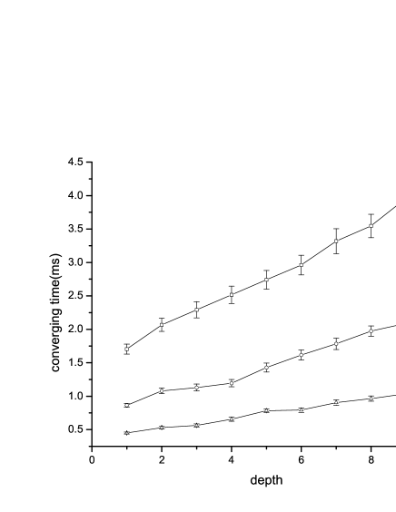
Figure 1: The converging time to synchronization under trees with different depth. All the trees are of the same size $N=10$. The only different between them is the depth of the tree. The $\square$ stands for the overall coupling strength $\sigma$ is 5, the $\bigcirc$ stands for $\sigma=10$ and the $\bigtriangleup$ stands for $\sigma=20$ .The result is averaged by 50 times.

To investigate which affects the converging time of the network, we adopt the trees with 10 nodes. When the depth is 1, the tree has only one root, all the other nodes which only receive input from the root are located in the second hierarchical level. When the depth of the tree is 9, the tree is just a chain connecting all the nodes. When the depth of the tree is from 2 to 8, the structures are more complicated. We compare the converging time of the trees with different depths. Since the trees with the same depth may have different structures, we use the average $T$ to represent the converging time. From Fig.1, it is clear that the deeper the tree is, the more converging time is needed to reach synchronized state. The effect of the depth to converging time is linear roughly.

Furthermore, given the depth, the converging time will not be affected by the size of the tree. It is reasonable because every branch of the tree is independent, and the longest branch will reach the synchronized state at last no matter how many the branches are. It can be seen from the compare between the trees from 10 nodes to 100 nodes from Fig.2. In the simulation, we keep the two kind of trees with the same depth such as 1, 5 and 9.

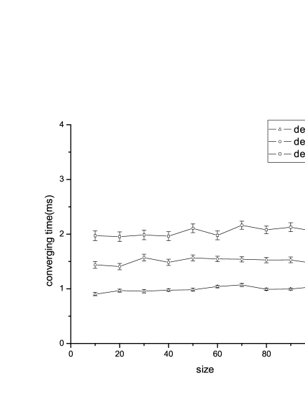
Figure 2: The converging time to synchronization under trees with different size. The overall coupling strength $\sigma$ is kept the same as 10. The $\triangle$ stands for the depth of the tree equals 1, the $\bigcirc$ stands for $depth=5$ and the $\Box$ stands for $depth=9$ .The result is averaged by 50 times.

So it is the depth of the tree that actually affects the converging time of the synchronization process. Additional, when given the depth of a tree, with specific oscillator model and overall coupling strength $\sigma$, the converging time is almost a constant. Since the initial state of each oscillator is given randomly, there may be some fluctuation in the constant, which can be described by the error. Thus, if we want to find a best way to distribute the weight to enhance the synchronization, we just have to look for the spanning tree with minimal depth. This kind of tree has minimal $R$ value and shortest converging time, which means that it has maximal synchronizability and efficiency.

2.2 Center of the network and the shortest spanning tree

To get such a tree is to create a shortest oriented tree from a undirected network. Each tree has a root, the root adopting is very important because it determines the depth of the tree. However, the root is not simply the node with the largest degree. For in some case, the spanning tree created by this root may be not the shortest. A typical example is shown in Fig.3. Here, we call the node to create the shortest spanning tree as the center of the network.

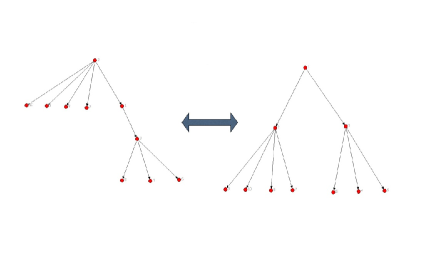
Figure 3: Given a network with 10 nodes, the left tree is created by adopting the node with largest degree as the root, and the right one is the shortest tree based on this topology. Obviously, the center is not simply the node with the largest degree.

We use the signaling process to find the center. For a network with $N$ nodes, every node is assumed to be a system which can send, receive, and record signals. A node can only affect its neighbors, which will affect their neighbors in the same way. Finally, each node will affect the whole network. At the beginning, we set every node as the source and give each of them one unit of signal, the signaling process is independent. For each step, the node will transmit the signal to the neighbors. For the signaling process is independent, several signal can be transmitted in a node simultaneously. After $m$ time steps, there must be a signal which covers all the nodes in the network with the fewest steps. So corresponding source node is the center of the network which is the root of the shortest spanning tree.

Actually, the above signaling process could be described by a simple but clear mathematical mechanism[25]. Suppose we have a network with $N$ nodes, it can be represented mathematically by an adjacency matrix $A$ with elements $A_{ij}$ equals to 1 if there is an edge from $i$ to $j$ and 0 otherwise. And the $I$ is a matrix where all the diagonal elements are 1 and others are 0. Then the column $i$ of matrix $V=(I+A)^{m}$ will represent the effect of source node $i$ to the whole network in $m$ steps. So we can get a $N$-dimensional vector that records each node’s signal quantity which represents the effect of the source node. If all the elements of a column are nonzero, the signal of the source node $i$ has affected the whole network. For each step, all the columns will be updated. To find the center, we should simply find which column reaches totally nonzero at first.

The shortest spanning tree can be created by the signaling process too. Suppose node $i$ is the center of the network, we mark $i$ as the used node. The second level includes all the unused nodes connected to the node $i$, then mark all these nodes and the edges from $i$ to them as used. To create the third level, we consider each node in the second level as sub-center, and the process is the same as the center $i$. Specifically, the edges between the nodes in the same level should be left unmarked. Moreover, if a node $k$ is marked by one of the node in the higher level, although the node $k$ is connected to another node $j$ in the higher level, the edge between $k$ and $j$ should be left unmarked too. After all the nodes are marked, we can get the shortest spanning tree. The nodes in the tree are connected by the marked edge and the direction of the edge is from the higher level to the lower level. This spanning tree (i) embeds a directed spanning tree, (ii) has no directed loop, and (iii) has normalized input strengths as the Ref[20]. So the index $R$ of the tree equals to 1. Additionally, For its depth is minimal in all spanning trees from the given network, so the synchronization converging time will be the shortest.

The topology of the original network is related to the depth of such effective directed trees. For instance, the center of the scale-free network usually has big degree. This kind of center can reduce the depth of the tree significantly. On the contrary, the homogenous random network does not have such kind of center, so the depth of the spanning tree from these networks will always be longer than that from the scale-free network as shown in Fig.4.

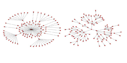
Figure 4: The left tree is a shortest spanning tree created from a scale-free network, which is from BA model with average degree 6. The right one is from a random network with the same average degree as the scale-free network. It clear that the depth of such effective directed trees is related to the topology of the original networks.

3 Conclusion

In the former works, to enhance the synchronization is always to reduce the index $R$. That is to reduce the overall coupling strength. However, the converging time is also an important factor. In this paper, we find that the depth of the tree is the only factor that effects the converging time when given the oscillator model and the overall coupling strength $\sigma$. Additionally, we present a simple way to obtain the shortest spanning tree with maximal synchronizability and efficiency from any given network.

In order to enhance the synchronizability of a network, the coupling strength of each edge is always be scaled by some structural characteristics such as degree, betweeness and so forth. The purpose of this process is to reduce the effect of the edges which is disadvantage for synchronization. To make the process to an extreme way, creating a spanning tree from a network is to cut off some edges in the network, which can also be considered as imposing the weight of these edges to 0. All the spanning trees from the network have the same $R=1$, which means the critical overall couple strength of the tree is minimal. Hence, the tree creating is a coupling strength scaling process.

Moreover, compared with any spanning tree from a given network, the shortest spanning tree can reduce the converging time significantly. It makes the tree have maximal efficiency. In fact, comparing with the former works[15-16], the way presented by us is universal. It is valid not only in the heterogeneous networks, but also in the homogenous networks.

References

- [1] T. Nishikawa, A. E. Motter, Y.-C. Lai, and F. C. Hoppensteadt, Phys. Rev. Lett. 91, 014101 (2003).
- [2] H. Hong, B. J. Kim, M. Y. Choi, and H. Park, Phys. Rev. E 69, 067105 (2004).
- [3] P. N. McGraw and M. Menzinger, Phys. Rev. E 72, 015101(R) (2005).
- [4] M. Zhao, T. Zhou, B.-H. Wang, G. Yan, H.-J. Yang, and W.-J.Bai, Physica A 371, 773 (2006).
- [5] X. Wu, B.-H. Wang, T. Zhou, W.-X. Wang, M. Zhao, and H.-J. Yang, Chin. Phys. Lett. 23, 1046 (2006).
- [6] D.J. Watts, S.H. Strogatz, Nature (London) 393, 440 (1998) .
- [7] M. Barahona, L.M. Pecora, Phys. Rev. Lett. 89, 054101 (2002).
- [8] H. Hong, B.J. Kim, M.Y. Choi, H. Park, Phys. Rev. E 69, 067105 (2004).
- [9] T. Nishikawa, A.E. Motter, Y.-C. Lai, F.C. Hoppensteadt, Phys. Rev. Lett. 91, 014101 (2003).
- [10] M.E.J. Newman, Phys. Rev. Lett. 89, 208701 (2002).
- [11] Adilson E.Motter, Changsong Zhou, and Jurgen Kurths, Phys. Rev. E 71, 016116 (2005).
- [12] M.Chavez, D.-U.Hwang, A.Amann, H.G.E.Hentschel, and S.Boccaletti, Phys. Rev. Lett. 94, 218701 (2005).
- [13] Changsong Zhou,Adilson E.Motter,and Jurgen Kurths, Phys. Rev. Lett. 96, 034101 (2006).
- [14] M.Zhao, T.Zhou, B.-H.Wang, Q.Ou, J.Ren, Eur. Phys. J. B 53, 375-379 (2006).
- [15] D.-U. Hwang, M. Chavez, A. Amann, S. Boccaletti, Phys. Rev. Lett. 94. 138701 (2005).
- [16] Y.-F. Lu, M. Zhao, T. Zhou, B.-H. Wang, Phys. Rev. E 76. 057103 (2007).
- [17] M. Barahona, L.M. Pecora, Phys. Rev. Lett. 89. 054101 (2002).
- [18] L.M. Pecora, T.L. Carroll, Phys. Rev. Lett. 80. 2109-2112 (1998).
- [19] K.S. Fink, G. Johnson, T. Carroll, D. Mar, L. Pecora, Phys. Rev. E 61.5080-5090 (2000).
- [20] T. Nishikawa, A.E. Motter, Phys. Rev. E 73. 065106 (2006).
- [21] Alex Arenas, Albert Diaz-Guilera, Jurgen Kurths, Yamir Moreno and Changsong Zhou, Physics Reports 469. 93-153 (2008).
- [22] A.T. Winfree. J. Theoret, Biol. 16. 15-42 (1967).
- [23] S.H. Strogatz, Physica D 143. 1-20 (2000).
- [24] J.A. Acebr n, L.L. Bonilla, C.J. P rez-Vicente, F. Ritort, R. Spigler, Rev. Mod. Phys. 77. 137-185 (2005).
- [25] Yanqing Hu, Menghui Li, Peng Zhang, Ying Fan, and Zengru Di, Phys. Rev. E 78, 016115 (2008).