The scaling of forced collisionless reconnection

Abstract

This paper presents two-fluid simulations of forced magnetic reconnection with finite electron inertia in a collisionless three-dimensional (3D) cube with periodic boundaries in all three directions. Comparisons are made to analogous two-dimensional simulations. Reconnection in this system is driven by a spatially localized forcing function that is added to the ion momentum equation inside the computational domain. Consistent with previous results in similar, but larger forced 2D simulations [B. Sullivan, B. N. Rogers, and M. A. Shay, Phys. Plasmas 12, 122312 (2005)], for sufficiently strong forcing the reconnection process is found to become Alfvénic in both 2D and 3D, $i.e.$, the inflow velocity scales roughly like some fraction of the Alfvén speed based on the upstream reconnecting magnetic field, and the system takes on a stable configuration with a dissipation region aspect ratio on the order of $0.15$.

I Introduction

Magnetic reconnection allows a magnetized plasma system to convert magnetic energy into high speed flows and thermal energy, and is the main driving mechanism behind energetic phenomena such as solar flares, magnetospheric substorms, and tokamak sawteeth. A defining feature of these phenomena is that they are very bursty: in a substorm, for example, a significant fraction of the lobe magnetic flux is reconnected over a period of about 10 minutes, while the time between periodic substorms is roughly 2.75 hours borovsky . Similarly, in the case of an X-class solar flare, the energy release may occur during several minutes or less in active regions that can last for weeks before reconnecting miller . A viable model of reconnection in such systems must therefore be consistent with the relatively long, quasi-stable periods in between reconnection bursts, as well as the rapidity of the energy release once a burst has somehow been triggered.

Regarding the rapidity of reconnection, recent research (see, $e.g.$, Refs. Birn01 ; BirnHesse01 ; Ma01 ; Bhattacharjee01 ; Pritchett01 ; Rogers01 ; Shay4 ; Zeiler02 ; Scholer03 ; Huba04 ; Fitzpatrick04 ; Ricci04 ; Shay04 ; Cassak ; Chacon07 ) has suggested that the reconnection process can indeed generate sufficiently fast rates of energy release to be consistent with observations provided that various conditions are met. For example, studies of spontaneous, unforced reconnection in systems with sufficiently narrow current sheets ($\delta\mathrel{\smash{\mathop{\raise 2.0pt\hbox{$<$}}\limits_{\smash{\raise 4.0pt\hbox{$\sim$}}}}\vphantom{\leq}}d_{i}=c/\omega_{pi}$ in the case without a guide magnetic field) have found that the reconnection process becomes Alfvénic - that is, the inflow velocity of plasma and magnetic flux into the reconnection region scales roughly like some fraction of the Alfvén speed based on the upstream reconnecting component of the magnetic field. The narrowing of the current layer down to widths $\delta\mathrel{\smash{\mathop{\raise 2.0pt\hbox{$<$}}\limits_{\smash{\raise 4.0pt\hbox{$\sim$}}}}\vphantom{\leq}}d_{i}$ serves as a trigger point for the onset of fast reconnection in this case due to the important role played by non-ideal effects such as the Hall term Birn01 . Without the addition of ad-hoc anomalous resistivity terms, simulations of systems with substantially thicker current sheets do not exhibit such fast reconnection behavior: at best the reconnection rates are throttled by the formation of long, narrow outflow layers as in the Sweet-Parker model, or in unfavorable magnetic geometries ($e.g.$ $\Delta^{\prime}\leq 0$  FKR ) no spontaneous reconnection may take place at all.

The fact that reconnection can occur very rapidly or not at all is consistent with the burstyness of the reconnection phenomena discussed earlier provided one can explain how a system can transition from a quasi-stable phase (characterized, for example, by a relatively thick current sheet) to a period of fast reconnection (a narrow current sheet). One possible mechanism to explain this transition is explored in this paper: to externally force a stable, thick current sheet system so that the magnetic flux and electric current are compressed in a localized region down to the small scales $\delta\mathrel{\smash{\mathop{\raise 2.0pt\hbox{$<$}}\limits_{\smash{\raise 4.0pt\hbox{$\sim$}}}}\vphantom{\leq}}d_{i}$ at which non-ideal effects such as the Hall term become important. This compression is generated in our simulations by a spatially localized external forcing term that is added to the ion momentum equation inside a three-dimensional (3D) computational domain. This method allows the scaling of the reconnection rate in 3D to be studied over a wide dynamic range: by changing the level of forcing, our simulations achieve more than an order of magnitude variation in the magnetic field just upstream of the reconnection region, and more than two orders of magnitude variation in the reconnection rate. The simulations show that such localized forcing in 3D can indeed induce fast rates of reconnection similar to those observed in 2D, spontaneously reconnecting, narrow current sheet systems, even in magnetic geometries that would not reconnect at all in the absence of forcing. This result - that a system with a locally narrow current sheet will exhibit fast reconnection behavior (whether the narrow current sheet is created by external forcing or is present initially) - is reasonable but not obvious, since the magnetic geometries outside the forced zone in the two cases may be very different.

This finding extends to 3D a similar result that was obtained in a larger 2D study Sullivan , as well as an earlier 2D multi-code study of forced reconnection known as the Newton Challenge NEWTON ; Pritchett05 ; Huba06 . The simulations in the Newton Challenge were initialized with a relatively narrow current sheet that was unstable to spontaneous reconnection but was somewhat thicker than the threshold required for fast (Alfvénic) reconnection (two ion skin depths compared to roughly one). The current sheet was then pinched by a spatially and temporally dependent inflow velocity imposed at the upstream boundary of the simulation domain. The result was that Alfvénic reconnection indeed occurred in all studies that included the Hall term, albeit with reconnection rates $\sim 20\%-50\%$ lower than those found in studies of spontaneous (unforced) reconnection in systems with somewhat narrower current sheets (one ion skin depth). The work described here goes beyond the Newton Challenge to explore, over a wide range of parameters, the scaling of forced magnetic reconnection in a tearing mode stable ($\Delta^{\prime}\leq 0$) system with an initially broad current sheet and a forcing function that is spatially localized in 3D.

Several limitations of the present work that are worth noting. Our simulations explore the dynamics of forced reconnection in a cubical box of 25.6 ion skin depths (the 3D analog of the GEM Challenge system Birn01 ) using a simple isothermal two-fluid model Shay4 and periodic boundary conditions. The frozen-in condition is broken at the smallest scales in this model by electron inertia and numerical diffusion effects. Particle simulations of reconnection, on the other hand, have shown that non-gyrotropic pressure tensor effects, which are not included here, should play the dominant role in this regard. Past 2D studies of unforced reconnection (see, for example, Refs. Birn01 ; BirnHesse01 ; Ma01 ; Bhattacharjee01 ; Pritchett01 ; Rogers01 ) have suggested that the reconnection rate is not strongly sensitive to this difference, and it is hoped that this insensitivity carries over to the present study. In addition, 2D particle simulations in much larger boxes are currently being used to study the sensitivity of the reconnection process to the boundary conditions and the physics of the electron diffusion region Bessho05 ; Karimabadi07 ; Shay07 ; Drake08 ; Pritchett08 . Due to the size limitations imposed by the 3D nature of our study, as well as the physical simplicity of our model, these important issues lie outside the scope of the present work.

The organization of this paper is as follows. In section II we describe the simulation model, equilibrium profiles, and forcing function. In section III we present and discuss the results of the simulations included in this study. The main conclusions are summarized in section IV.

II Simulation Model

Our simulations are based on the two-fluid equations with the addition of a spatially localized forcing term in the ion momentum equation. These equations in normalized form are Shay04 :

$$n\left(\partial_{t}\mathbf{V}_{i}+\mathbf{V}_{i}\cdot\nabla\mathbf{V}_{i}\right)=\mathbf{J}\times\mathbf{B}-\nabla p+F_{y}\hat{\mathbf{y}}$$ (1)

$$\partial_{t}\mathbf{B}^{\prime}=-\nabla\times\mathbf{E}^{\prime}$$ (2)

$$\mathbf{E}^{\prime}+\mathbf{V}_{i}\times\mathbf{B}=\frac{1}{n}\left(\mathbf{J}\times\mathbf{B}^{\prime}-\nabla p_{e}\right)$$ (3)

$$\partial_{t}n+\mathbf{V}_{i}\cdot\nabla n=-n\nabla\cdot\mathbf{V}_{i}$$ (4)

$$p_{e}=nT_{e}\ ,\quad p_{i}=nT_{i}\ ,\quad p=p_{i}+p_{e}$$ (5)

$$\mathbf{B}^{\prime}=\left(1-\frac{m_{e}}{m_{i}}\nabla^{2}\right)\mathbf{B}\ ,\mathbf{V}_{e}=\mathbf{V}_{i}-\mathbf{J}/n\ ,\mathbf{J}=\nabla\times\mathbf{B}$$ (6)

Here $F_{y}=F_{y}(x,y,z,t)$ is the forcing function, the form of which is discussed in below. For simplicity we assume an isothermal equation of state for both electrons and ions (qualitatively similar to the adiabatic case), and thus take $T_{e}$ and $T_{i}$ to be constant. The normalizations of Eqns. (1)-(6) are based on constant reference values of the density $n_{0}$ and the reconnecting component of the magnetic field $B_{x0}$, and are given by (normalized $\to$ physical units): $t\to\omega_{ci}t$, $\omega_{ci}=eB_{x0}/(m_{i}c)$, $x\to x/d_{i}$, $d_{i,e}=c/\omega_{pi,e}$, $\omega_{pi,e}^{2}=4\pi n_{0}e^{2}/m_{i,e}$, $n\to n/n_{0}$, $\mathbf{B}\to\mathbf{B}/B_{x0}$, $\mathbf{V}_{i,e}\to\mathbf{V}_{i,e}/V_{Ax}$, $V_{Ax}=\omega_{ci}d_{i}=B_{x0}/(4\pi n_{0}m_{i})^{1/2}$, $T_{i,e}\to T_{i,e}4\pi n_{0}/B_{x0}^{2}$, $p_{i,e}\to p_{i,e}4\pi/B_{x0}^{2}$, $\mathbf{J}\to\mathbf{J}/(n_{0}eV_{Ax})$, and $F_{y}\to F_{y}d_{i}/(m_{i}n_{0}V_{Ax}^{2})$. Our algorithm employs fourth-order spatial finite differencing and the time stepping scheme is a second-order accurate trapezoidal leapfrog zalesak1 ; zalesak2 . We consider a cubical 3D simulation box with physical dimensions $L\times L\times L=25.6d_{i}\times 25.6d_{i}\times 25.6d_{i}$ (so that $L=25.6$ in normalized units) and periodic boundary conditions imposed at $x=\pm L/2$,$y=\pm L/2$, and $z=\pm L/2$ . The simulation grid is $n_{x}\times n_{y}\times n_{z}=128\times 256,\times 128$, yielding grid scales of $\Delta_{x}=\Delta_{z}=0.2$ and $\Delta_{y}=0.1$. The electron to ion mass ratio is $m_{e}/m_{i}=1/25$ so that the normalized electron skin depth is $d_{e}=\sqrt{m_{e}/m_{i}}=0.2$. The frozen-in law for electrons is broken primarily by the presence of finite electron inertia, which is manifested by the $m_{e}$ terms in the definition of $B^{\prime}$ in Eq. (6). Very near the x-points, however, the electron inertia terms become weak in quasi-steady conditions, since both the $\partial_{t}$ and $\mathbf{v}\cdot\nabla$ terms on the left-hand-side of Eq. (1) become small. In these small regions the frozen-in law is mainly broken by numerical diffusion. Past studies of this effect (e.g. Ref. Rem ) have found that the rates of reconnection are relatively insensitive to such grid-level diffusion and are in reasonable agreement with the rates obtained from particle simulations Uzdensky00 .

II.1 Initial Equilibrium

We begin with a one dimensional equilibrium. Three dimensional effects will enter via the forcing function described in the next section. The normalized magnetic field and density profiles in our initial equilibrium are given by:

$$\mathbf{B}(y) = \sin\left[\frac{2\pi}{L}\left(y+\frac{L}{4}\right)\right]\mathbf{\hat{x}}$$ (7)

$$n(y) = 1+\frac{1-B_{x}^{2}}{2(T_{i}+T_{e})}$$ (8)

The boundary conditions are periodic in all three directions. As required by these boundary conditions, $B$ is periodic under $y\to y+L$. Note that the normalization parameter $B_{x0}$ has been chosen so that the peak value of this initial field is unity. From the given form of $n$ it is apparent that $n=1$ at this location, or in physical units, $n=n_{0}$. The density profile is chosen to satisfy the total pressure balance condition, which in normalized form is given by

$$n(T_{i}+T_{e})+\frac{1}{2}B_{x}^{2}={\rm constant}$$ (9)

Unless otherwise stated, we take the (constant) total temperature to be $T_{tot}=T_{i}+T_{e}=1.0$, or in physical units $4\pi n_{0}T_{tot}/B_{x0}^{2}=1$, so that the plasma $\beta$ based on the reconnecting field has a (minimum) value of 2 where $B_{x}=1$ and $n=1$. The density reaches a maximum value of $n=1.5$ in the center of the equilibrium current sheets ($y=\pm L/4$) where $B_{x}=0$. Initially the current is carried entirely by the electrons, while the ions begin at rest. To prevent energy buildup at the grid scale, the simulations include fourth order dissipation in the density and momentum equations of the form $\mu_{4}\nabla^{4}$ where $\mu_{4}=5.1\cdot 10^{-5}$. To avoid physically artificial effects that can arise from exact reflection symmetries of the initial condition, a small amount of random noise is added to the magnetic field and ion current at the levels $|\tilde{B}_{max}|\approx 10^{-4}$, $|\tilde{J}_{i_{max}}|\approx 10^{-4}$.

The linear tearing mode stability parameter is defined as $\Delta^{\prime}=[\partial_{y}\tilde{\psi}(y\to 0+)-\partial_{y}\tilde{\psi}(y\to 0-)]/\tilde{\psi}(y=0)$ where $\tilde{\psi}$ is the perturbation in flux the function FKR . In our system it is given by Ott :

$$\Delta^{\prime}(k_{x})=-\left(2k_{0}\sqrt{\frac{k_{x}^{2}}{k_{0}^{2}}-1}\right)\tan\left(\sqrt{\frac{k_{x}^{2}}{k_{0}^{2}}-1}\right),$$ (10)

where $k_{0}=2\pi/L$. Since periodicity along the $x$ direction requires $k_{x}\geq 2\pi/L$ and thus $k_{x}^{2}/k_{0}^{2}\geq 1$, one sees that $\Delta^{\prime}\leq 0$. Therefore, as noted in the introduction, the system we consider is stable to tearing modes in the absence of forcing and exhibits no spontaneous reconnection.

II.2 Forcing Function

The initial 1D equilibrium described in the previous section does not contain a pre-seeded x-line. Rather, we employ a forcing function to drive plasma and magnetic flux into the region surrounding the point $(x,y,z)=(L/4,-L/4,0)$, thereby forming an x-line along z through that location. The forcing function has the general form $F_{y}(x,y,t)=X(x)Y(y)Z(z)\Theta(t)$. Along x and z the forcing function is a gaussian with widths $w_{x}$ and $w_{z}$, respectively, centered at $(x,z)=(+L/4,0)$:

$$\begin{split}X(x)&=\exp\left\{-\left[\frac{(x-L/4)}{w_{x}/2}\right]^{2}\right\},\\ Z(z)&=\exp\left\{-\left(\frac{z}{w_{z}/2}\right)^{2}\right\}\end{split}$$ (11)

Along the inflow ($y$) direction, the forcing function is antisymmetric in $y$ about $y=-L/4$. It varies linearly with $y$ close to the reconnection point and then levels off to a constant value ($Y\to\pm 1$) over a distance of $\sim 2w_{y}$ upstream of the x-point:

$$Y(y)=\tanh\left(\frac{y-L/4}{w_{y}}\right)-\tanh\left(\frac{y+L/4}{w_{y}}\right)+1$$ (12)

The temporal behavior of the forcing is controlled by the function $\Theta(t)$. This function starts at zero and increases monotonically with time at the rate $d\Theta/dt\sim 1/\tau_{f}=0.1$ until it plateaus at the value $F_{\infty}$:

$$\Theta(t)=F_{\infty}\tanh\left(\frac{t}{|F_{\infty}|\tau_{f}}\right)$$ (13)

Since the initial slope of $\Theta(t)$ and hence the initial rate of ramping is held constant at $1/\tau_{f}=0.1$ from one simulation to the next, it takes more time to ramp up to the stronger levels of forcing (roughly $\tau\sim|F_{\infty}|\tau_{f}$).

In our simulations the spatial and temporal structure of the forcing is controlled by the parameters $w_{x},w_{y},w_{z},\tau_{f}$, and $F_{\infty}$. The appropriate choice of these parameters presumably varies from system to system, depending on the physical application under consideration and the nature of the forcing agent. In this study, as a first step, we examine the reconnection behavior as a function of the asymptotic strength of the forcing function $F_{\infty}$, holding the other forcing function parameters fixed at values that are convenient for the size of our simulations, $e.g.$ $w_{x}=w_{z}=5.0d_{i},\tau_{f}=1.25\omega_{ci}^{-1}$ . In the substantially larger system considered in Ref. Sullivan , the authors employed a proportionally broader forcing function with results similar to those described here. The detailed study of how the geometry of the forcing function impacts the reconnection is left for future work.

III Numerical Results

This study includes ten simulations. Five are two dimensional and differ from each other only in the asymptotic level of forcing $F_{\infty}$. These five simulations are included as a baseline for comparison with the other five, which are three dimensional with forcing localized as a gaussian in the out of plane direction. In the 3D simulations, the width of the forcing function along $z$ is equal to its width along $x$ ($w_{x}=w_{z}=5.0d_{i}$). In the next section we will describe the results of a typical 2D run and then compare to a similar 3D case. First, however, some important definitions are required.

Following Ref. Shay04 and our previous 2D work Sullivan , we focus on the ion inflow $V_{in}\ (=V_{y})$, outflow $V_{out}\ (=V_{x})$, upstream reconnecting magnetic field $B_{d}\ (=B_{x})$, and upstream density $n_{d}$, near the boundaries of the ion dissipation region where the ions decouple from both the electrons and the magnetic field. As found in earlier work Sullivan , the ion and electron velocities typically decouple approximately $0.5c/\omega_{pi}$ upstream of the x-point below the center of the forcing function, and we therefore measure the upstream quantities $V_{in}$, $B_{d}$, and $n_{d}$ at this location $(+L/4,-L/4\pm 0.5,0)$. The reconnecting component of the magnetic field does not vary strongly as a function of $y$ between 0.5 and 1.0 ion skin depths upstream of the x-point; therefore, the results presented here are not strongly dependent upon the method used to determine the upstream edge of the dissipation region. This holds in both 2D and 3D.

The electron outflow ($i.e.$ outflow in the x-direction) typically becomes quite large very close to the x-point and can be in excess of the ion Alfvén speed. However, at the downstream edge of the dissipation region, the electrons slow down to flow roughly with the ions. The location where the two flows come together is typically close to the location of the maximum in $V_{ix}$. Therefore the downstream edge of the dissipation region is taken to be the location of the maximum in $V_{ix}$. Defining the downstream edge as the location of the ion-electron velocity crossover point yields nearly identical results Shay04 ; Sullivan .

A last important definition concerns the reconnection rate. In 2D, the reconnection rate is defined as the time derivative of the reconnected magnetic flux inside the magnetic island per unit length in the (uniform) $z$ direction:

$$R_{0}=\frac{\partial}{\partial t}\int_{x_{o}}^{x_{x}}B_{y}(x,-L_{y}/4)dx,$$ (14)

where $y=-L/4$ is the plane where $B_{x}=0$, and $x_{{}_{X}}$, $x_{{}_{O}}$ are the x-locations of the x-point and o-point, respectively. A total reconnection rate (rather than a rate per unit length) cannot be defined in the 2D limit, since the uniformity of the system along $z$ implies that the total reconnected flux is infinite. This is not the case in the 3D simulations discussed here, in which the extent of the magnetic island and the total reconnected flux are both finite in the $z$ direction. Thus in 3D it is natural to define the reconnection rate as simply the time derivative of the total reconnected flux inside the magnetic island:

$$R_{tot}=\frac{\partial}{\partial t}\int_{A}B_{y}dx\ dz$$ (15)

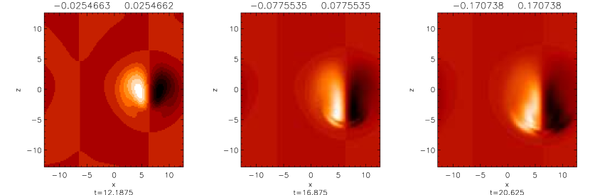
where $A$ is the area of the magnetic island (found numerically using field-line tracing) in the central plane of the equilibrium current sheet $y=-L_{y}/4$. Fig. (1) shows a time series $B_{y}$ in this plane in a simulation discussed in the next section. The location of the forcing function, centered at $(x,z)=(6.4,0)$, can be discerned from the dipolar signature in the right half of the figures. As we show below, nearly all the reconnected flux is inside this roughly circular region under the forcing function. (In both 2D and 3D, small secondary islands are also typically present; however, the total flux in these islands is small and they have no significant impact on the reconnection rates reported here.) The 3D reconnection rate given by Eq. (15) has physical units of [flux/time], in contrast to Eq. (14), which has physical units of [flux/time/length]. To compare the 2D and 3D reconnection rates, the 3D rate therefore must be somehow translated into a reconnection rate per unit length, as in 2D. No unique way exists to do this, making a meaningful comparison of the 2D and 3D reconnection rates difficult. Two crude approaches to such a comparison, however, are discussed further in the following section.

Figure 1: (color online) Time evolution of $B_{y}(x,z)$ at $t=12.1875$ (left), $t=16.875$ (center), and $t=20.625$ (right). The reconnected flux moves in the $-z$ direction. Maximum and minimum values of the plotted quantity are shown above each plot.

III.1 Temporal Behavior

Fig. (2) shows time series of the dissipation region parameters in typical 2D (left) and 3D (right) simulations. In the 2D simulation, the asymptotic upstream forcing strength is $F_{\infty}=0.15$, as seen from the solid curve in Fig. (2g). Note the level of forcing has become constant by $t\approx 3$. In panel (a), we plot the outflow velocity (dashed curve), and 5 times the inflow velocity (dotted curve) in the 2D case (the factor of 5 serves to place the quantities on a similar scale). As the forcing is turned on, the inflow velocity increases, causing the pressure and density (panel c) to mount under the forcing function. This back pressure causes the inflow velocity to level off and then decrease around $t\approx 4.5$. Magnetic flux also piles up under the forcing function causing the upstream field to increase, as seen in panel (e) during the period $t<12$. Consistent with past studies ($e.g.$ Refs.  Shay04 ; Sullivan ; Cassak ), at about $t\sim 12$, when the flux pile-up has narrowed the current sheet to about an ion skin depth, the layer opens up into a Petschek-like configuration and fast reconnection begins, as can be seen by the rise in the reconnection rate $R_{0}$ in panel (g). This onset of reconnection causes $V_{in}$ to increase again and $B_{d}$ to level off, indicating that the rate of reconnection is sufficient to prevent further pile up of upstream flux, $i.e.$ flux is liberated from the dissipation region by reconnection at a rate comparable to that with which flux is pumped into the region, so that $B_{d}$ is stable for an extended period ($t\sim 10-25$). The ratio $V_{in}/V_{out}\sim 0.1-0.2$ in this phase is consistent with continuity arguments: Assuming in the 2D case that the ion diffusion region has a width $2\delta$ and a length $2D$, the approximate incompressibility of the ion flow yields $V_{in}D\sim V_{out}\delta$ or $V_{in}/V_{out}\sim\delta/D$. As shown in Fig. (3), the value of $\delta/D$ is typically between 0.1 - 0.2. Here $\delta/D$ is computed by dividing the half-width at half-max of the current sheet at the location of the x-line by the distance from the x-line to the location of the peak ion outflow velocity along $x$. The aspect ratio varies somewhat in time, approaching some minimum value then generally becoming slightly larger again as the current sheet opens up and shortens into a Petschek-like configuration.

Figure 2: Time series of the dissipation region parameters in 2D(left) and 3D(right) with $F_{\infty}=0.15$, and $0.2$, respectively.

Strong reconnection continues in the 2D system for about another $10$ time units beyond the final time ($t=25$) shown in the figures, at which point the system runs out of magnetic flux to reconnect and the reconnection rate drops sharply to zero. The features described here are observed at all levels of forcing in 2D that are sufficiently strong to trigger Alfvénic reconnection. In Ref. Sullivan qualitatively similar results were found in a larger ($L\times L=102.4d_{i}\times 102.4d_{i}$) 2D system.

Figure 3: Time series of the aspect ratio of the dissipation region vs. time in 2D (solid curve) and 3D (dashed curve. (Same simulations as the data shown in Fig.( 2))

Several differences are apparent in comparing the 2D data shown in left half of Fig. (2) with the 3D data in the right half. For example, the enhancement in the density (panel d) and upstream magnetic field (panel f) are weaker or more gradual in 3D than in 2D. This results from a key difference between 2D and 3D: in 2D flux can compress upstream of the current sheet or it can reconnect, flowing out along $x$. Similarly, density can build up under the forcing function or it can be cleared out by reconnection. In 3D, plasma and magnetic flux have the option of either reconnecting or flowing away from the forced zone along the $\pm z$ directions. This difference has at least two important consequences: first, the forcing function is not as effective at compressing plasma and flux in 3D. Indeed, the gradual rise in $B_{d}$ seen in Fig. (2f) results largely from the convection of stronger upstream magnetic field into the reconnection zone rather than from in-situ compression. To partially compensate for this, in Fig. (2) we compare 2D and 3D simulations with somewhat different levels of forcing ($F_{\infty}=0.2$ in 3D vs. $F_{\infty}=0.15$ in 2D as shown in Figs. (2g,h)). A second consequence, which we discuss further below, is that the reconnection “efficiency” in 3D is smaller than in 2D – that is, a smaller fraction of the upstream magnetic flux that is initially contained within the forced region is reconnected in 3D than in 2D, making the reconnecting phase of the 3D simulations shorter than those in the 2D runs.

Two measures of the reconnection rate are shown in Fig. (2h). The dotted curve labeled $R_{0}$, like panel (g), is the integral given by Eq. (14) calculated in the $z=0$ plane. This quantity is a rough measure of the rate of reconnection immediately under the center of the forcing function. Although one might expect this $z=0$ location to yield the largest local reconnection rate, in fact substantially larger values can occur at negative $z$ values near the edge of the forced zone. This can be seen from Fig. (4), which shows the $z$-dependence of the reconnected flux per unit $z$ [Eq. (14) without the time derivative] at various times. The area under the curves at a given time yields the total reconnected flux [Eq. (15) without the time derivative]. The flux distributions become skewed to the left at later times due to the dragging of the magnetic field by the electrons. This leftward electron flow carries the bulk of the (rightward) electric current density that supports the reversal in the reconnecting magnetic field $J_{z}\propto dB_{x}/dy$. The transport of reconnected flux by the electron flow can also be seen in the downward drift of the $B_{y}$ profile in the center of the sheet shown in Fig. (1). This effect has also been reported in other studies of three-dimensional reconnection (see, for example, Refs. Rudakov02 ; Huba02 ; Hesse05 ; Lapenta06 ). A second measure of the reconnection rate is shown as the dashed curve in Fig. (2h) labeled $R_{tot}/10$. This curve depicts the total reconnection rate $R_{tot}$ given by Eq. (15) divided by the full width of the forcing function along $z$ ($2w_{z}=10.0d_{i}$). As can be seen from Fig. (4), this width roughly characterizes the extent along $z$ of the reconnected flux distribution and thus $R_{tot}/10$ is a crude measure of the average reconnection rate per unit length in the 3D system. Although the reconnection rates as characterized by these measures are somewhat smaller in the 3D system than those in the 2D case, we show in the the following section that, when the 2D and 3D reconnection rates are plotted as a function of the instantaneous values of the upstream reconnecting magnetic field [Figs. (2e,f)], similar results are obtained. That is, for a given value of the upstream magnetic field, the rates of reconnection characterized by either $R_{0}$ or $R_{tot}/10$ are roughly comparable to the corresponding 2D values.

Figure 4: Time evolution of the reconnected flux per unit z as a function of z (solid curves), and the shape of the forcing function(dashed curve).

Another feature apparent in the 3D data of Fig. (2) is the downturn in the reconnection rate (panel h) and upstream field (panel f) seen at $t\simeq 23$. At this time, nearly all of the magnetic flux in the forced zone has been expelled by the forcing function, and thus the system has effectively run out of flux to reconnect. This is much earlier than the otherwise similar collapse in the 2D reconnection rate at $t\simeq 38$. As was noted earlier, less flux is reconnected in 3D because the plasma and magnetic field are free to flow outward along the $\pm z$ directions without reconnecting. In 2D, the uniformity of the system along $z$ prevents any net transport of flux in that direction, and a much larger fraction of the initial upstream flux in 2D (over 70% percent compared to about 10% in 3D) ends up inside the magnetic islands at late times.

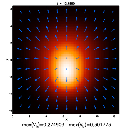
A final difference between 2D and 3D evident from Figs.(2a,b) is that the ratio $V_{in}/V_{out}$ in 3D is enhanced by roughly a factor of two over the 2D case. Given that the layer aspect ratio $\delta/D$ [Fig. (3)] shows a much smaller increase, this enhancement is inconsistent with the 2D continuity argument described earlier, $V_{in}/V_{out}\sim\delta/D$. In the 3D simulations, however, the continuity relation must be modified by a geometric factor. In 2D, the ion outflow from the reconnection region is almost entirely along the $x$ direction with $V_{ix}\gg V_{iz}$. In 3D, as one can see from the snapshot shown in Fig. (5), the ion outflow is nearly omnidirectional with $V_{iz}\sim V_{ix}$, and the ion diffusion region is disk-shaped (like a hockey puck) rather than rectangular. Assuming this disk has radius $D$ and half-thickness $\delta$, plasma will thus flow into an area $A_{in}=\pi D^{2}$ (one surface of the disk) and out through an area $A_{out}=2\pi D\delta$. Continuity then demands that $V_{in}A_{in}=V_{out}A_{out}$ or

$$V_{in}=\left(\frac{A_{out}}{A_{in}}\right)V_{out}=\left(\frac{2\pi D\delta}{\pi D^{2}}\right)V_{out}=\left(\frac{2\delta}{D}\right)V_{out}.$$ (16)

Thus, for the same aspect ratio $\delta/D$, one would expect $V_{in}/V_{out}$ to be a factor of two larger in the 3D case, as indeed it is.

III.2 Scaling of Reconnection

In this section we test two simple scaling relations for the plasma outflow and reconnection rate that have been found in past studies to characterize reconnection in some forced and unforced 2D systems ($e.g.$ Shay99 ; Shay04 ; Huba04 ; Shay98b ; Hesse99 ; Birn01 ; Shay01 ; Sullivan ). In the case of the outflow, the dynamics that cause reconnected field lines to accelerate plasma away from the x-point are similar to those of an Alfvén wave, and so $V_{out}\sim V_{Ad}$ where $V_{Ad}=B_{d}/\sqrt{4\pi m_{i}n}$. Regarding the reconnection rate, for a given dissipation region of length $D$ and thickness $\delta$, the continuity arguments discussed in the last section yield $V_{in}\sim C_{0}(\delta/D)V_{Ad}$ where $C_{0}\sim 1$ in 2D and $C_{0}\sim 2$ in 3D. Assuming this inflow along $y$ carries an $x$-directed magnetic field $B_{d}$ into the dissipation region, the rate of reconnection per unit length along $z$ (equivalent to the rate at which magnetic flux enters the reconnection zone per unit length along $z$) is $V_{in}B_{d}$. We therefore expect:

$$V_{out} \sim\left(\frac{\delta}{D}\right)\frac{B_{d}}{\sqrt{4\pi m_{i}n}}$$ (17a)

$$R_{0} \sim V_{in}B_{d}\sim\left(\frac{C_{0}\delta}{D}\right)\frac{B_{d}^{2}}{\sqrt{4\pi m_{i}n}}\ .$$ (17b)

Note the reconnection rate $R_{0}$ is predicted to scale with the square of the upstream field. In normalized units, isolating the upstream field $B_{d}$ as the independent variable, these become

$$V_{out}n^{1/2} \sim\left(\frac{\delta}{D}\right)B_{d}$$ (18a)

$$R_{0}^{1/2}n^{1/4} \sim\left(\frac{C_{0}\delta}{D}\right)^{1/2}B_{d}$$ (18b)

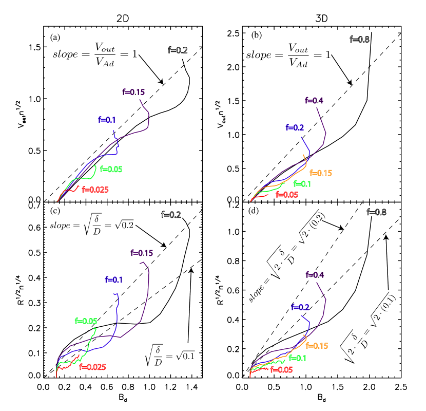
We now test these scaling laws under the assumption that $\delta/D$ has an approximately constant value (on the order of 0.1 - 0.2) over the duration of the Alfvénic phase of the reconnection process. In Figs.  (6a,b), to test the validity of Eq. (18a), the quantity $V_{out}\sqrt{n_{d}}$ is plotted versus $B_{d}$ with time as a parameter. Each curve represents data from a single simulation and is labeled by the value of $F_{\infty}$ for that simulation. A sixth 2D simulation with $F_{\infty}=0.025$ is included to extend the range of data. (This weakest level of forcing is insufficient to produce Alfvénic reconnection in 3D, so no 3D analog for this simulation is included.) The dotted line of slope unity, plotted for reference, represents an outflow velocity equal to the upstream Alfvén speed based on $B_{d}$. At the stronger forcing levels, the data are indeed in rough agreement with the predicted scaling, albeit with significant, order-unity time variations within any given simulation. At the weakest forcing levels, the outflow (like the reconnection rate discussed in a moment) falls below the predicted scaling. The forcing strength in these simulations is insufficient to narrow the current sheet down to the ion skin depth scale, and fast reconnection is never triggered.

Figure 5: (color online) The gray scale plot in this figure shows $J_{z}$ in the central plane of the forced current sheet at $t=12.188$ in the 3D simulation with $F_{\infty}=0.2$. The over-plotted vectors (blue online) show the relative magnitude and direction of $\mathbf{V}_{i}=\mathbf{J}_{i}/n$ in the same plane.

In Figs. (6c,d), the quantity $R_{0}^{1/2}n_{d}^{1/4}$ is plotted vs. $B_{d}$ to test the scaling of the reconnection rate given by Eq. (18b). Plots based on $R_{tot}/10$ rather than $R_{0}$ yield slightly larger but similar results. The dotted lines represent the expected scaling, assuming that $V_{out}/V_{A}=1.0$ and that the system has an unvarying dissipation region aspect ratio of $(\delta/D)=1/5$ (steeper line) or $(\delta/D)=1/10$ (less steep). At the later times when the reconnection rates are highest, the data in the more strongly forced simulations roughly follow the expected trend. In the most weakly forced runs, however, the scaling progressively breaks down; the perturbation of the current sheet in these cases is insufficient to trigger fast reconnection before a nearly force-balanced state is reached.

IV Conclusions

We have examined the scaling behavior of reconnection in a forced, three-dimensional, periodic system using two-fluid simulations with finite electron inertia. The forcing in the simulations was driven by a spatially localized forcing function added to the ion momentum equation inside the computational domain. We initialized the system with a one dimensional, broad current sheet equilibrium that was tearing-mode stable; three dimensional structure entered through the localization of the forcing function. Comparisons were made to analogous two-dimensional simulations.

In the two dimensional case, as found our previous work in larger 2D systems Sullivan , sufficiently strong levels of forcing were found to produce a quasi-steady Petschek-like reconnection configuration with a dissipation region aspect ratio $\delta/D\sim 0.1-0.2$. The forcing function produces a pileup of magnetic flux in the upstream region and hence an increase in the upstream magnetic field, until the reconnection rate becomes sufficient to prevent further pileup of magnetic flux. The flux pile-up typically halts once a relatively thin current sheet is formed—between 0.5 and 1.0 ion skin depths in width—at which point the magnetic separatrix opens up, and fast, Alfvénic reconnection begins, leading to a period when the upstream reconnecting field $B_{d}$ is relatively stable. The rate of reconnection per unit length along the (ignorable) $z$ direction was found to scale roughly like $B_{d}^{2}$, as expected from simple scaling arguments, although significant time variations are observed during the course of any given run than cannot be explained by this simple scaling.

Figure 6: (color online) (a) $V_{out}\sqrt{n}$ vs. $B_{d}$ in 2D, (b) $V_{out}\sqrt{n}$ vs. $B_{d}$ in 3D , (c) $\sqrt{R_{0}}\sqrt[4]{n}$ vs. $B_{d}$ in 2D, (d)$\sqrt{R_{0}}\sqrt[4]{n}$ vs. $B_{d}$ in 3D

In three dimensions, freedom of the plasma to flow out in the $\pm z$ directions makes the forcing function less effective at compressing plasma; the resulting flux pile-up is weaker in 3D, convection dominates over compression in the upstream region, and the period of reconnection is shorter than in comparable 2D systems. The localization of the magnetic island along $z$ in 3D makes it possible to define a total reconnection rate, rather than a rate per unit length, as in 2D. For sufficiently strong forcing, this total rate, like in 2D result, was found to be roughly proportional $B_{d}^{2}$.

To directly compare the 2D and 3D reconnection rates one must translate the 3D rate into a rate per unit $z$, as in 2D. Two rough methods of extracting such a quasi-2D rate from the 3D data were described – one of which is simply to divide the total rate in 3D by the width of the forcing function – with similar results. When either of these two rates are plotted as a function of the upstream magnetic field, the 2D and 3D results are comparable. On the other hand, the distribution of reconnected magnetic flux in 3D becomes strongly skewed at late times by the flow of electrons in the current layer, and near the edge of the forcing function, the flux builds at local rates that can substantially exceed the 2D values.