Critical point of the two-dimensional Bose gas: an S-matrix approach

Abstract

A new treatment of the critical point of the two-dimensional interacting Bose gas is presented. In the lowest order approximation we obtain the critical temperature $T_{c}\approx 2\pi n/[m\log(2\pi/mg)]$, where $n$ is the density, $m$ the mass, and $g$ the coupling. This result is based on a new formulation of interacting gases at finite density and temperature which is reminiscent of the thermodynamic Bethe ansatz in one dimension. In this formalism, the basic thermodynamic quantities are expressed in terms of a pseudo-energy. Consistent resummation of 2-body scattering leads to an integral equation for the pseudo-energy with a kernel based on the logarithm of the exact 2-body S-matrix.

I Introduction

The properties of interacting Bose gases can be very different depending on the spatial dimension. This has become especially interesting in recent years due to the possibility of experimentally realizing lower dimensional cold gases with magnetic and optical traps. In 3 dimensions there is a critical point for Bose-Einstein condensation (BEC) even in the non-interacting theory, with a critical temperature $T_{c}=4\pi\left(n/\zeta(3/2)\right)^{2/3}$ where $n$ is the density and $\zeta$ Riemann’s zeta function. In two dimensions the same formula becomes $T_{c}=4\pi n/\zeta(1)$ and since $\zeta(1)$ diverges there is no critical point at finite temperature for the non-interacting gas. It is believed however that the two-dimensional interacting gas has a critical point in the universality class of the Kosterlitz-Thouless transition rather than BECPopov ; Fisher ; Baym ; Prokofev . (For a review see Posaz .) This transition has recently been observed in experimentsKruger .

In the one-dimensional case the particles effectively behave as fermions, the model is integrable, and an exact solution is known based on the thermodynamic Bethe ansatz (TBA)Lieb ; YangYang . The one-dimensional case illustrates the importance of non-perturbative methods like the TBA for understanding the physics. Whereas the usual perturbative finite-temperature Feynman diagram method involving Matsubara frequencies in loops is a standard approach which entangles zero temperature perturbation theory with quantum statistical sums, the TBA represents an entirely different organization of the free energy which essentially disentangles the two. More specifically, the only property of the model it is based on is the exact 2-body scattering matrix computed to all orders in perturbation theory at zero temperature. In principle a TBA-like organization of the free energy is possible for non-integrable theories in any dimension based on the formula in Ma which expresses the partition function in terms of the exact S-matrix. The derivation of the TBA as given by Yang and Yang however was not based on the result in Ma but rather relied on the factorizability of the multi-particle S-matrix into 2-body S-matrices for integrable systems. For non-integrable systems the formalism in Ma can be quite complicated since the free energy contains N-body terms which do not factorize. Nevertheless, for a dilute gas the consistent resummation of the 2-body scattering terms can represent a useful approximation that is intrinsically different from other methods.

In this work we derive explicit expressions for the free-energy, occupation numbers, etc., in this 2-body approximation for non-integrable models in any spatial dimension. The result is TBA-like: everything is expressed in terms of a pseudo-energy that satisfies an integral equation with a momentum-dependent kernel which is related to a matrix element of the logarithm of the S-matrix. Our analysis builds on the previous workLeclair , and the final result presented here contains several important technical improvements.

Most of this paper is devoted to developing the formalism in generality. In section III we describe contributions to the free energy with diagrams, not to be confused with finite temperature Feynman diagrams, where the vertices represent $N$-body interactions for any $N$. The cluster decomposition of the S-matrix is necessary to establish the extensivity of the free energy. In section IV we derive an integral equation for the occupation numbers (filling fractions) from a variational principle based on a Legendre transformation that exchanges the chemical potential with the filling fraction. In section V we present the integral equation that consistently resums the infinite number of 2-body diagrams. In section VI the 2-body kernel that appears in the integral equation is derived for interacting Bose gases in 2 and 3 dimensions. In section VII we compare our approximation to the exact TBA for the 1-dimensional case.

This new formalism is illustrated in the 2-dimensional case. Since the 2-body approximation is reasonably simple in its final form, we present a self-contained analysis of the critical point of the Bose gas in the next section, where we derive an expression for the coupling constant dependent critical density.

II Critical point of the two-dimensional Bose gas

In this section we illustrate the main ingredients of our formalism by applying it to the critical point of the two-dimensional Bose gas. Our treatment is significantly different from previous onesPopov ; Fisher ; Baym ; Prokofev . Although we find results that are similar to the known results, we find our treatment to be considerably simpler and transparent and doesn’t rely on an effective description of vortices. As will become clear, the full power of our formalism is actually unnecessary to obtain these results when the coupling is very small. We set $\hbar=k_{B}=1$ unless otherwise indicated.

The interacting Bose gas in 2 spatial dimensions is defined by the following hamiltonian:

$$H=\int d^{2}{\bf x}\left({1\over 2m}|\vec{\nabla}\phi(x)|^{2}+{g\over 4}|\phi(x)|^{4}\right)$$ (1)

where $\phi$ is a complex field and $m$ is the mass of the particles. In two dimensions, the combination $mg/\hbar^{2}$ is dimensionless; in the experiment Kruger it is approximately $0.13$.

In the formalism developed in the sequel, the occupation numbers, or filling fractions, are expressed in terms of a pseudo-energy $\epsilon({\bf k})$, and the density has the following form:

$$n=\int{d^{2}{\bf k}\over(2\pi)^{2}}{1\over e^{\beta\epsilon({\bf k})}-1}$$ (2)

where $\beta$ is the inverse temperature $T$. In an approximation that consistently resums all the 2-body interactions, the pseudo-energy satisfies the integral equation in eq. (66) where the kernel $G_{2}({\bf k},{\bf k}^{\prime})$ is related to a logarithm of the exact 2-body scattering matrix and given explicitly in eq. (80), for convenience reproduced here:

$$G_{2}({\bf k}_{1},{\bf k}_{2})=-{8\over m}\arctan\left({mg/8\over 1+{mg\over 8\pi}\log\left({4\Lambda^{2}\over|{\bf k}_{1}-{\bf k}_{2}|^{2}}\right)}\right)$$ (3)

where $\Lambda$ is an ultra-violet cut-off. When the coupling $g$ is small, the kernel is small and the eq. (66) can be approximated by:

$$\epsilon({\bf k})=\omega_{\bf k}-\mu-\int{d^{2}{\bf k}^{\prime}\over(2\pi)^{2}}\,G_{2}({\bf k},{\bf k}^{\prime}){e^{\beta(\epsilon_{{\bf k}^{\prime}}-\omega_{{\bf k}^{\prime}}+\mu)}\over e^{\beta\epsilon_{{\bf k}^{\prime}}}-1}$$ (4)

where $\mu$ is the chemical potential and $\omega_{\bf k}={\bf k}^{2}/2m$ is the single particle energy.

Since when $g=0$, $\epsilon({\bf k})=\omega_{\bf k}-\mu$, an approximate solution to (4) is obtained by substituting $\epsilon({\bf k})=\omega_{\bf k}-\mu$ on the right hand side. As in Bose-Einstein condensation, the critical point is defined to occur at the value of the chemical potential $\mu_{c}$ where the occupation number at zero momentum diverges, i.e. $\epsilon({\bf k}=0)=0$. This gives the following integral equation for $\mu_{c}$:

$$\mu_{c}=-\int{d^{2}{\bf k}\over(2\pi)^{2}}\,G_{2}(0,{\bf k}){1\over e^{\beta(\omega_{\bf k}-\mu_{c})}-1}$$ (5)

At very weak coupling, to leading order we can neglect the momentum dependence of the kernel and simply take $G_{2}=-g$. Consider first the case where the interaction is attractive, i.e. $g<0$. The equation (5) becomes

$$\beta\mu_{c}=-{mg\over 2\pi}\log\left(1-e^{\beta\mu_{c}}\right)$$ (6)

For negative $g$, the above equation has negative $\mu_{c}$ solutions, which makes physical sense since energy is released when a particle is added. Here the attractive interaction makes a critical point possible at finite temperature and density. The critical density $n_{c}\approx\mu_{c}/g$.

Suppose now the attraction is repulsive, i.e. $g>0$. The equation (6) now has no real solutions for $\mu_{c}$. This can be traced to the infra-red divergence of the integral when $\mu_{c}$ changes sign. Let us therefore introduce a low-momentum cut-off $k_{0}$, i.e. restrict the integral to $|{\bf k}|>k_{0}$. The equation (5) now becomes

$$\beta\mu_{c}={mg\over 2\pi}\left[\beta\epsilon_{0}-\beta\mu_{c}-\log\left(e^{\beta(\epsilon_{0}-\mu_{c})}-1\right)\right]$$ (7)

where $\epsilon_{0}=k_{0}^{2}/2m$. The above equation now has solutions at positive $\mu_{c}$, however for arbitary $k_{0}$ there are in general two solutions. If $k_{0}$ is chosen appropriately to equal a critical value $k_{c}$, then there is a unique solution $\mu_{c}$. This is shown in Figure 1, where the right and left hand sides of equation (7) are plotted against $\mu_{c}$ for two values of $k_{0}$, one being the critical value $k_{c}$. Since the slopes of the right and left hand sides of eq. (7) are equal at the critical point, taking the derivative with respect to $\mu_{c}$ of both sides gives the additional equation:

$$\beta(\epsilon_{c}-\mu_{c})=\log\left(1+{mg\over 2\pi}\right)$$ (8)

where $\epsilon_{c}=k_{c}^{2}/2m$. The two equations (7, 8) determine $\mu_{c}$ and $\epsilon_{c}$:

$$\mu_{c} = {mgT\over 2\pi}\log\left(1+{2\pi\over mg}\right)$$ (9)

$$\epsilon_{c} = {k_{c}^{2}\over 2m}=T\left(1+{mg\over 2\pi}\right)\log\left(1+{mg\over 2\pi}\right)+{mgT\over 2\pi}\log\left({2\pi\over mg}\right)$$ (10)

Note that $\epsilon_{c}$ goes to zero as $g$ goes to zero. Finally, making the approximation $\epsilon({\bf k})\approx\omega_{\bf k}-\mu_{c}$ in eq. (2) and using eq. (7) one obtains the critical density $n_{c}\approx\mu_{c}/g$:

$$n_{c}\approx{mk_{B}T\over 2\pi\hbar^{2}}\log\left(1+{2\pi\over mg}\right)$$ (11)

The above can be expressed as $n_{c}\lambda^{2}=\log(1+2\pi/mg)$ where $\lambda=\hbar\sqrt{2\pi/mk_{B}T}$ is the thermal wavelength. As expected, at fixed density, the critical density goes to infinity as $g$ goes to zero.

\psfrag{Y}{RHS, LHS}\psfrag{X}{$\beta\mu_{c}$}\psfrag{xc}{$\epsilon_{0}=\epsilon_{c}$}\psfrag{xo}{$\beta\epsilon_{0}=0.9$}\includegraphics[width=284.52756pt]{mucrit.eps}

Figure 1: Left and right hand sides of eq. (7) as a function of $\beta\mu_{c}$ at two values of the infra-red cut-off $\epsilon_{0}$, one being the critical value $\epsilon_{c}$.

In obtaining the above result we have only kept the leading term in the kernel $G_{2}$ at small coupling, which is momentum-independent. Systematic corrections to the above results may be obtained by keeping higher order terms in the kernel. However since the kernel involves $\log{\bf k}^{2}$, at small coupling these corrections are quite small, as we have verified numerically.

In numerical simulations of the critical point, it was found that $\mu_{c}\sim{mgT\over 2\pi}\log(2C/mg)$ where $C$ is a constantProkofev . This form agrees with our result (9) in the limit of small $g$, however, whereas we find $C=\pi$, numerically one finds a significantly higher value $C\approx 13.2$. Assuming that $C$ was not overestimated numerically, one possible explanation for this discrepancy is based on the renormalization group. The beta-function for $g$ can be found by requiring that the kernel $G_{2}$ in eq. (80) be independent of the ultra-violet cut-off $\Lambda$. To lowest order this gives:

$$\Lambda{dg\over d\Lambda}={mg^{2}\over 4\pi}$$ (12)

which implies the coupling decreases at low energies. Integrating this equation leads to the cut-off dependent coupling $g(\Lambda)$:

$${2\pi\over mg(\Lambda)}={2\pi\over mg_{0}}\left(1+{mg_{0}\over 4\pi}\log(\Lambda_{0}/\Lambda)\right)$$ (13)

where $g_{0}=g(\Lambda_{0})$. Thus at low energies where $\Lambda<\Lambda_{0}$, the combination $2\pi/mg$ grows. However since the dependence on the cut-off is only logarithmic, it is not clear that this could explain the large $C$ discrepancy. This seems to imply that higher N-body interactions are important.

III Partition function in terms of the S-matrix

III.1 Formal expression for $Z$ in terms of the S-matrix

We are interested in the partition function:

$$Z(\beta,\mu)=\rm Tr~{}e^{-\beta(H-\mu N)}$$ (14)

where $\beta=1/k_{B}T$ and $\mu$ is the chemical potential. We henceforth set $k_{B}=1$. The trace will be performed over the free particle Fock space. Assuming only one kind of particle, the trace is computed based on the following resolution of the identity:

$${\bf 1}=\sum_{N=0}^{\infty}{1\over N!}\int(d{\bf k}_{1})\,(d{\bf k}_{2})\cdots(d{\bf k}_{N})~{}~{}|{\bf k}_{1}\cdots{\bf k}_{N}\rangle\langle{\bf k}_{1}\cdots{\bf k}_{N}|$$ (15)

where $(d{\bf k})\equiv d^{d}{\bf k}/(2\pi)^{d}$ and $d$ is the spatial dimension. We adopt the following conventions:

$$|{\bf k}_{1},\ldots,{\bf k}_{N}\rangle=a^{\dagger}_{{\bf k}_{1}}\cdots a^{\dagger}_{{\bf k}_{N}}\,|0\rangle$$ (16)

$$a_{\bf k}a^{\dagger}_{\bf k^{\prime}}~{}-s~{}a^{\dagger}_{\bf k^{\prime}}a_{\bf k}=(2\pi)^{d}\,\delta^{(d)}({\bf k}-{\bf k^{\prime}})$$ (17)

where $s=1$ corresponds to bosons and $s=-1$ fermions. For simplicity we will use the following notation: $\delta_{{\bf k},{\bf k}^{\prime}}\equiv\delta^{(d)}({\bf k}-{\bf k}^{\prime})$. The energy of a free one-particle state will be denoted as $\omega_{\bf k}$. We will also need:

$$\delta_{{\bf k},{\bf k}}=\delta^{(d)}(0)={V\over(2\pi)^{d}}$$ (18)

where $V$ is the volume.

As usual, we assume the hamiltonian can be split into a free part $H_{0}$ and an interacting part: $H=H_{0}+H_{I}$. Let $\widehat{S}(E)$ denote the S-matrix operator in the formal theory of scattering where $E$ is an off-shell energy variable. It can be expressed in the conventional manner:

$$\widehat{S}(E)=1+2\pi i\,\delta(E-H_{0})\,\widehat{T}(E)$$ (19)

where $H_{0}$ is the free hamiltonian operator and everywhere the over-hat denotes a quantum operator. On shell the matrix elements of $\widehat{T}(E)$ are $T=(2\pi)^{d}\delta_{\{{\bf k},{\bf k}^{\prime}\}}{\cal M}_{\{{\bf k}\}\to\{{\bf k}^{\prime}\}}$ where ${\cal M}$ are the scattering amplitudes.

Our starting point is the basic formula derived in Ma :

$$Z=Z_{0}+{1\over 4\pi i}\int_{0}^{\infty}dEe^{-\beta E}\rm Tr\left(\widehat{S}^{-1}{{\stackrel{{\scriptstyle\leftrightarrow}}{{\partial}}}}_{E}\widehat{S}\right)$$ (20)

where $X{{\stackrel{{\scriptstyle\leftrightarrow}}{{\partial}}}}_{E}Y=X(\partial_{E}Y)-(\partial_{E}X)Y$, and $Z_{0}$ is the free partition function. We will work with the equivalent expression:

$$Z=Z_{0}+{1\over 2\pi}\int dE\,{\rm e}^{-\beta E}\,\rm Tr\,{\rm Im}\,\partial_{E}\log\widehat{S}(E)$$ (21)

Since $\log\widehat{S}(E)\propto\delta(E-H_{0})$, let us define the operator $W$ as follows:

$${\rm Im}\log\widehat{S}(E)\equiv 2\pi\delta(E-H_{0})\,W(E)$$ (22)

Integrating by parts, one then has

$$Z=\int dE\,{\rm e}^{-\beta E}\,\rm Tr\left(\delta(E-H_{0})(W(E)\beta+1)\right)$$ (23)

The advantage of the above expression is that in taking the trace, $H_{0}$ can be replaced with the free particle energies and the integral over $E$ performed. For simplicity of notation, define

$$\widehat{W}\equiv W\beta+1$$ (24)

III.2 Cluster decomposition

As we will see, clustering properties of the S-matrix ensure that the free energy depends only on connected matrix elements and is proportional to the volume. For any operator $X$, the cluster decomposition can be expressed as follows:

$$\langle\Psi^{\prime}|X|\Psi\rangle=\sum_{\rm partitions}s^{p}~{}\langle\Psi^{\prime}_{1}|X|\Psi_{1}\rangle_{c}\langle\Psi^{\prime}_{2}|X|\Psi_{2}\rangle_{c}\langle\Psi^{\prime}_{3}|X|\Psi_{3}\rangle_{c}\cdots$$ (25)

where the sum is over partitions of the state $|\Psi\rangle$ into clusters $|\Psi_{1}\rangle,|\Psi_{2}\rangle,....$. (The number of particles in $|\Psi_{i}\rangle$ and $\langle\Psi^{\prime}_{i}|$ is not necessarily the same.) The above formula essentially defines what is meant by the connected matrix elements $\langle X\rangle_{c}$.

In order for the free energy to be extensive, $\widehat{W}$ must cluster properly, as we now describe. Introducing the short-hand notation $|{\bf{12}}\cdots\rangle=|{\bf k}_{1}{\bf k}_{2}\cdots\rangle$, for the operator $\widehat{W}$ the above equation reads

$$\langle{\bf 1^{\prime}}|\widehat{W}|{\bf 1}\rangle = \langle{\bf 1^{\prime}}|\widehat{W}|{\bf 1}\rangle_{c}$$ (26)

$$\langle{\bf 1^{\prime}2^{\prime}}|\widehat{W}|{\bf 12}\rangle = \langle{\bf 1^{\prime}2^{\prime}}|\widehat{W}|{\bf 12}\rangle_{c}+\langle{\bf 1^{\prime}}|\widehat{W}|{\bf 1}\rangle_{c}\langle{\bf 2^{\prime}}|\widehat{W}|{\bf 2}\rangle_{c}+s\langle{\bf 2^{\prime}}|\widehat{W}|{\bf 1}\rangle_{c}\langle{\bf 1^{\prime}}|\widehat{W}|{\bf 2}\rangle_{c}$$

$$\langle{\bf 1^{\prime}2^{\prime}3^{\prime}}|\widehat{W}|{\bf 123}\rangle = \langle{\bf 1^{\prime}2^{\prime}3^{\prime}}|\widehat{W}|{\bf 123}\rangle_{c}$$

$$~{}~{}~{}~{}+\left[\langle{\bf 1^{\prime}}|\widehat{W}|{\bf 1}\rangle_{c}\langle{\bf 2^{\prime}3^{\prime}}|\widehat{W}|{\bf 23}\rangle_{c}+{\rm permutations}\right]_{9}$$

$$~{}~{}~{}~{}~{}~{}~{}~{}~{}~{}+\left[\langle{\bf 1^{\prime}}|\widehat{W}|{\bf 1}\rangle_{c}\langle{\bf 2^{\prime}}|\widehat{W}|{\bf 2}\rangle_{c}\langle{\bf 3^{\prime}}|\widehat{W}|{\bf 3}\rangle_{c}+{\rm permutations}\right]_{6}$$

etc. The subscript $[*]_{9}$ denotes the number of terms within the bracket, so that for 3 particles there is a total of $1+9+6=16$ terms on the right hand side of the above equation. The connected matrix elements are characterized by being proportional to a single overall $\delta$-function.

When $\{{\bf k}^{\prime}\}=\{{\bf k}\}$, the above cluster expansion leads to another specialized type of cluster expansion that is suited to the computation of the partition function. From eq. (26) we define $\widehat{w}_{N}({\bf k}_{1},...,{\bf k}_{N})$ as factors that cannot be written as a product of separate functions of disjoint subsets of the ${\bf k}_{i}$:

$$\langle{\bf 1}|\widehat{W}|{\bf 1}\rangle = \langle{\bf 1}|\widehat{W}|{\bf 1}\rangle_{c}=\widehat{w}_{1}({\bf k}_{1})$$ (27)

$$\langle{\bf 12}|\widehat{W}|{\bf 12}\rangle = \widehat{w}_{2}({\bf k}_{1},{\bf k}_{2})+\widehat{w}_{1}({\bf k}_{1})\widehat{w}_{1}({\bf k}_{2})$$

$$\langle{\bf 123}|\widehat{W}|{\bf 123}\rangle = \widehat{w}_{3}({\bf k}_{1},{\bf k}_{2},{\bf k}_{3})+\Bigl{[}\widehat{w}_{2}({\bf k}_{2},{\bf k}_{3})\widehat{w}_{1}({\bf k}_{1})+\widehat{w}_{2}({\bf k}_{1},{\bf k}_{3})\widehat{w}_{1}({\bf k}_{2})+\widehat{w}_{2}({\bf k}_{1},{\bf k}_{2})\widehat{w}_{1}({\bf k}_{3})\Bigr{]}$$

$$~{}~{}~{}~{}~{}~{}~{}~{}~{}~{}~{}~{}~{}~{}~{}~{}~{}~{}~{}~{}~{}~{}~{}~{}~{}~{}~{}~{}~{}+\widehat{w}_{1}({\bf k}_{1})\widehat{w}_{1}({\bf k}_{2})\widehat{w}_{1}({\bf k}_{3})$$

etc. The above definition implies that the $\widehat{w}_{N}$ are sums of terms involving the connected matrix elements of $\widehat{W}$. For instance:

$$\widehat{w}_{2}({\bf k}_{1},{\bf k}_{2}) = \langle{\bf 12}|\widehat{W}|{\bf 12}\rangle_{c}+s\langle{\bf 2}|\widehat{W}|{\bf 1}\rangle_{c}\langle{\bf 1}|\widehat{W}|{\bf 2}\rangle_{c}$$ (28)

$$\widehat{w}_{3}({\bf k}_{1},{\bf k}_{2},{\bf k}_{3}) = \langle{\bf 123}|\widehat{W}|{\bf 123}\rangle_{c}+\Bigl{[}s\langle{\bf 2}|\widehat{W}|{\bf 1}\rangle_{c}\langle{\bf 13}|\widehat{W}|{\bf 23}\rangle_{c}+{\rm perm.}\Bigr{]}_{6}$$

$$~{}~{}~{}~{}~{}~{}~{}+\Bigl{[}\langle{\bf 3}|\widehat{W}|{\bf 1}\rangle_{c}\langle{\bf 1}|\widehat{W}|{\bf 2}\rangle_{c}\langle{\bf 2}|\widehat{W}|{\bf 3}\rangle_{c}+{\rm perm.}\Bigr{]}_{2}$$

A combinatoric argument then shows:

$$\log Z=\sum_{N=1}^{\infty}{z^{N}\over N!}\int(d{\bf k}_{1})\cdots(d{\bf k}_{N})~{}{\rm e}^{-\beta\sum_{i=1}^{N}\omega_{i}}\,\widehat{w}_{N}({\bf k}_{1},...,{\bf k}_{N})$$ (29)

where $z\equiv e^{\beta\mu}$ and $\omega_{i}=\omega_{{\bf k}_{i}}$.

All of the $\widehat{w}$ are proportional to an overall $(2\pi)^{d}\delta^{(d)}(0)=V$, so let us factor out the volume $V$ and define:

$$\widehat{w}_{N}({\bf k}_{1},...,{\bf k}_{N})\equiv V\,w_{N}({\bf k}_{1},...,{\bf k}_{N})$$ (30)

The free energy density is then completely determined by the functions $w_{N}$:

$${\cal F}=-{1\over\beta V}\log Z=-{1\over\beta}\sum_{N=1}^{\infty}{z^{N}\over N!}\int(d{\bf k}_{1})\cdots(d{\bf k}_{N})~{}{\rm e}^{-\beta\sum_{i}\omega_{i}}\,w_{N}({\bf k}_{1},...,{\bf k}_{N})$$ (31)

For free particles, the only non-zero connected matrix element is the 1-particle to 1-particle one: $\langle 2|\widehat{W}|1\rangle=\langle 2|1\rangle$. This still implies $\widehat{w}_{N}$ is non-zero for any N:

$$\widehat{w}_{N}(1,2,..,N)=s^{N-1}(N-1)!\,\langle{\bf N}|{\bf 1}\rangle\langle{\bf 1}|{\bf 2}\rangle\langle{\bf 2}|{\bf 3}\rangle\cdots\langle{\bf N-1}|{\bf N}\rangle$$ (32)

Note that although $\widehat{w}_{N}$ is a product of N $\delta$-functions, it only has a single $\delta(0)$. All but one ${\bf k}$ integral is saturated by $\delta$-functions at each $N$ and one obtains the well-known free-particle result:

$${\cal F}_{0}={s\over\beta}\int{d^{d}{\bf k}\over(2\pi)^{d}}~{}\log\left(1-sze^{-\beta\omega_{\bf k}}\right)$$ (33)

III.3 Diagrammatic description

In the interacting case, terms involving the one-particle factors $\langle{\bf 2}|\widehat{W}|{\bf 1}\rangle_{c}$ can be easily summed over as in the free particle case. We assume that $|{\bf k}\rangle$ is a stable one-particle eigenstate of $H$ with energy $\omega_{\bf k}$:

$$\langle{\bf k}^{\prime}|\widehat{W}|{\bf k}\rangle_{c}=\langle{\bf k}^{\prime}|{\bf k}\rangle=(2\pi)^{d}\delta_{{\bf k},{\bf k}^{\prime}}$$ (34)

Consider for example the $\widehat{w}_{3}$ contribution coming from the second terms in eq. (28):

$$\log Z=....+{z^{3}\over 3!}\int(d{\bf k}_{1})(d{\bf k}_{2})(d{\bf k}_{3})\,{\rm e}^{-\beta\sum_{i=1}^{3}\omega_{i}}\,\left(s\langle{\bf 2}|\widehat{W}|{\bf 1}\rangle_{c}\langle{\bf 13}|\widehat{W}|{\bf 23}\rangle_{c}+{\rm perm.}\right)+...$$ (35)

Because of the $\delta$-function, one can do one ${\bf k}$ integral. Combined with the primary term coming from $\widehat{w}_{2}$ one finds:

$$\log Z=...+{z^{2}\over 2}\int(d{\bf k}_{1})(d{\bf k}_{2})\,{\rm e}^{-\beta(\omega_{1}+\omega_{2})}\,\left(1+sz(e^{-\beta\omega_{1}}+e^{-\beta\omega_{2}})\right)~{}\langle{\bf 12}|\widehat{W}|{\bf 12}\rangle_{c}+...$$ (36)

It is easy to see that the terms in the higher $\widehat{w}_{N}$ that involve one $\widehat{w}_{2}$ and $N-1$ $\widehat{w}_{1}$’s contribute additional terms in the parentheses of the above equation that sum up to $\prod_{i=1}^{2}(1-sze^{-\beta\omega_{i}})^{-1}$. To summarize this result in the most convenient way, define $\sum^{\prime}_{N}$ as the sum over $\widehat{w}_{N}$ terms minus any terms involving the 1-particle factors $\widehat{w}_{1}$. Then

$${\cal F}={\cal F}_{0}-{1\over\beta}{\sum_{N\geq 2}}^{\prime}{1\over N!}\int\left(\prod_{i=1}^{N}(d{\bf k}_{i})f_{0}({\bf k}_{i})\right)~{}w_{N}({\bf k}_{1},...,{\bf k}_{N})$$ (37)

where ${\cal F}_{0}$ is the free contribution in eq. (33) and we have defined the free “filling fraction”:

$$f_{0}({\bf k})\equiv{z\over e^{\beta\omega_{\bf k}}-sz}$$ (38)

The functions $w_{N}$ have many contributions built out of the connected matrix elements of $\widehat{W}$. Define the vertex function ${\cal V}({\bf k}_{1}^{\prime},...,{\bf k}_{m}^{\prime};{\bf k}_{1},...,{\bf k}_{n})$ as follows:

$$\langle{\bf k}_{1}^{\prime},...,{\bf k}_{m}^{\prime}|\widehat{W}|{\bf k}_{1},...,{\bf k}_{n}\rangle_{c}=\beta(2\pi)^{d}\delta_{{\bf k},{\bf k}^{\prime}}\,{\cal V}({\bf k}_{1}^{\prime},...,{\bf k}_{m}^{\prime};{\bf k}_{1},...,{\bf k}_{n})$$ (39)

The vertices ${\cal V}$ have no temperature dependence and are essentially on-shell matrix elements of $\log\widehat{S}$. To lowest order in the scattering matrix $\widehat{T}$, this vertex is just the scattering amplitude: ${\cal V}={\cal M}$. In the sequel we will compute ${\cal V}_{2}$ for the interacting Bose gas. Given our present interest in non-relativistic systems, only the matrix elements with $n=m$ are of concern here. We highlight this fact by attaching a subscript $n$ to ${\cal V}$:

$${\cal V}_{n}({\bf k}_{1}^{\prime},...,{\bf k}_{n}^{\prime};{\bf k}_{1},...,{\bf k}_{n})\equiv{\cal V}({\bf k}_{1}^{\prime},...,{\bf k}_{n}^{\prime};{\bf k}_{1},...,{\bf k}_{n})$$ (40)

Each term in the corrections ${\cal F}-{\cal F}_{0}$ can be represented graphically. We stress that this diagramatic expansion as defined here, while being analogous to the usual Feynman diagrams, is completely unrelated to the (finite temperature) Feynman diagram approach. This is clear since each vertex in principle represents an exact zero-temperature quantity summed to all orders in perturbation theory. The correction ${\cal F}-{\cal F}_{0}$ is the sum of all connected “vacuum diagrams”, made of oriented lines and vertices with $n$ incoming and $n$ outgoing lines attached, $n$ being any positive integer. Note that there must be at least one vertex; i.e. the circle isn’t allowed since it is already included as ${\cal F}_{0}$. A diagram is then evaluated according to the following rules and represents a contribution to ${\cal F}$:

1. Each line carries some momentum ${\bf k}$. To such a line is associated a factor of $f_{0}({\bf k})$.

2. To each vertex, with the incoming set and the outgoing set of momenta being $\{{\bf k}_{1},\dots,{\bf k}_{n}\}$ and $\{{\bf k}_{1}^{\prime},\dots,{\bf k}_{n}^{\prime}\}$ respectively, associate a factor of the vertex function $(2\pi)^{d}\beta\,{\cal V}_{n}({\bf k}_{1}^{\prime},...,{\bf k}_{n}^{\prime};{\bf k}_{1},...,{\bf k}_{n})$.

3. Enforce momentum conservation at each vertex.

4. Integrate over all unconstrainted momenta with $d^{d}{\bf k}/(2\pi)^{d}$.

5. Divide by the symmetry factor of the diagram, defined as the number of permutations of the internal lines that do not change the topology of the graph, including relative positions. This factor is identical to the usual symmetry factor of a Feynman diagram.

6. For fermions, include one statistical factor $s=-1$ for each loop.

7. Divide the result by the volume of space $V=(2\pi)^{d}\delta(0)$ and by $\beta$. Note that this is equivalent to dividing the space-time volume $V\beta$ since at finite temperature, $\beta$ is the circumference of compactified time.

The structure of this diagrammatic expansion is very similar to that in the work of Lee and YangLeeYang , however the vertices are different in the two approaches.

To illustrate this diagrammatic expansion, we will now describe the first few terms. There is only one diagram that has two lines, as shown in Figure 2. This diagram corresponds to:

$${\cal F}=....{1\over 2}\int(d{\bf k}_{1})(d{\bf k}_{2})f_{0}({\bf k}_{1})f_{0}({\bf k}_{2}){\cal V}_{2}({\bf k}_{1},{\bf k}_{2};{\bf k}_{1},{\bf k}_{2}).$$ (41)

Comparing with the expression (37), we identify $w_{2}({\bf k}_{1},{\bf k}_{2})=\beta{\cal V}_{2}({\bf k}_{1},{\bf k}_{2};{\bf k}_{1},{\bf k}_{2})$.

Figure 2: (a) Contribution to $w_{2}$. (b) Contribution to $w_{3}$.

At the next order, there is again only one diagram consisting of three lines, shown in Figure 2, and this implies $w_{3}({\bf k}_{1},{\bf k}_{2},{\bf k}_{3})=s\beta{\cal V}_{3}({\bf k}_{1},{\bf k}_{2},{\bf k}_{3};{\bf k}_{1},{\bf k}_{2},{\bf k}_{3})$.

Figure 3: Diagrams contributing to $w_{4}$

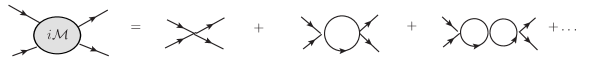
There are multiple diagrams with four lines, one of them includes ${\cal V}_{4}$, and the others can be built from ${\cal V}_{2}$. They are shown in Figure 3. Their sum is

$${\cal F}=...+\int \left[\prod_{i=1}^{4}(d{\bf k}_{i})f_{0}({\bf k}_{i})\right]\Bigl{[}{1\over 4!}{\cal V}_{4}({\bf k}_{1},\dots\bf k_{4};{\bf k}_{1},\dots\bf k_{4})$$

$$+ {s\over 2}(2\pi)^{d}\delta({\bf k}_{2}-{\bf k}_{3})\beta{\cal V}_{2}({\bf k}_{1},{\bf k}_{2};{\bf k}_{1},{\bf k}_{3}){\cal V}_{2}({\bf k}_{2},{\bf k}_{4};{\bf k}_{3},{\bf k}_{4})$$

$$+ {s\over 8}(2\pi)^{d}\delta(\sum_{i=1}^{4}{\bf k}_{i})\beta^{2}{\cal V}_{2}({\bf k}_{1},{\bf k}_{2};{\bf k}_{3},{\bf k}_{4}){\cal V}_{2}({\bf k}_{3},{\bf k}_{4};{\bf k}_{1},{\bf k}_{2})\Bigr{]}.$$

From this expression, we can identify $w_{4}$, which is now a sum of terms built from the vertices ${\cal V}_{4},{\cal V}_{2}$.

An interesting class of diagrams are the “ring-diagrams” shown in Figure 3, since they can be summed up in closed form. Let us define

$$G_{2}({\bf k},{\bf k}^{\prime})={\cal V}_{2}({\bf k},{\bf k}^{\prime};{\bf k},{\bf k}^{\prime})$$ (43)

A ring diagram with $N$ external rings attached will have the following value according to the diagrammatic rules:

$${1\over\beta N}s^{N+1}\int(d{\bf k}_{0})\prod_{i=1}^{N}(d{\bf k}_{i})\left[\beta G_{2}({\bf k}_{0},{\bf k}_{i})f_{0}({\bf k}_{i})\right]f_{0}({\bf k}_{0})^{N} N>1$$ if ; (44)

$${1\over 2\beta}\int(d{\bf k}_{0})(d{\bf k}_{1})\beta G_{2}({\bf k}_{0},{\bf k}_{1})f_{0}({\bf k}_{1})f_{0}({\bf k}_{0}) N=1$$ if .

Apart from the $N=1$ term which has a different coefficient, all other terms can be identified with the power series for the logarithmic function. This class of diagrams are then resummed into:

$${\cal F}_{\rm ring} = -{s\over\beta}\int(d{\bf k}_{0})\log\left(1-sf_{0}({\bf k}_{0})\int(d{\bf k}_{1})\beta G_{2}({\bf k}_{0},{\bf k}_{1})f_{0}({\bf k}_{1})\right)$$

$$~{}~{}~{}~{}~{}\quad-{1\over 2}\int(d{\bf k}_{0})(d{\bf k}_{1})G_{2}({\bf k}_{0},{\bf k}_{1})f_{0}({\bf k}_{1})f_{0}({\bf k}_{0})$$

Figure 4: Ring diagrams.

IV Legendre transformation and integral equation

IV.1 Generalities

Given ${\cal F}(\mu)$, one can compute the thermally averaged number density $n$:

$$n=-{\partial{\cal F}\over\partial\mu}\equiv\int(d{\bf k})~{}f({\bf k})$$ (46)

The dimensionless quantities $f$ are called the filling fractions or occupation numbers. One can express ${\cal F}$ as a functional of $f$ with a Legendre transformation. Define

$$G\equiv{\cal F}(\mu)+\mu\,n$$ (47)

Treating $f$ and $\mu$ as independent variables, then using eq. (46) one has that $\partial_{\mu}G=0$ which implies it can be expressed only in terms of $f$ and satisfies $\delta G/\delta f=\mu$. Inverting the above construction shows that there exists a functional $\digamma(f,\mu)$

$$\digamma(f,\mu)=G(f)-\mu\int(d{\bf k})f({\bf k})$$ (48)

which satisfies eq. (46) and is a stationary point with respect to $f$:

$${\delta\digamma\over\delta f}=0$$ (49)

The above stationary condition is to be viewed as determining $f$ as a function of $\mu$. The physical free energy is then ${\cal F}=\digamma$ evaluated at the solution $f$ to the above equation. We will refer to eq. (49) as the saddle point equation since it is suggestive of a saddle point approximation to a functional integral. The function $\digamma$ is also required to satisfy

$${\partial\digamma\over\partial\mu}=-\int(d{\bf k})\,f({\bf k})$$ (50)

In the sequel, it will be convenient to trade the chemical potential $\mu$ for the variable $f_{0}$. We will need:

$${\partial f_{0}\over\partial\mu}=\beta f_{0}(1+sf_{0})$$ (51)

In the free theory the functional $\digamma_{0}$ is fixed only up to the saddle point equations, thus its explicit expression is not unique. As we will see, the appropriate choice that is consistent with the diagramatic expansion is:

$$\digamma_{0}(f,f_{0})=-{1\over\beta}\int(d{\bf k})\left(s\log(1+sf)-\left({f-f_{0}\over 1+sf_{0}}\right)\right)$$ (52)

(This is different than the choice made in Leclair .) The saddle point equation ${\delta\digamma_{0}\over\delta f}=0$ implies $f=f_{0}$, and inserting this back into $\digamma_{0}$ gives the correct free energy ${\cal F}_{0}$ for the free theory. Furthermore, $\digamma_{0}$ satisfies eq. (50) if one uses the saddle point equation $f=f_{0}$.

Let us now include interactions by defining

$$\digamma=\digamma_{0}+\digamma_{1}$$ (53)

where $\digamma_{0}$ is given in eq. (52) and we define $U$ as the “potential” which depends on $f$ and incorporates interactions:

$$\digamma_{1}=-{1\over\beta}\int(d{\bf k})~{}U(f({\bf k}))$$ (54)

IV.2 Integral equation

The physical filling fraction $f$ can be obtained by differentiating ${\cal F}$ in (37) with respect to the chemical potential $\mu$, and the result is

$$f({\bf k})=f_{0}({\bf k})+f_{0}({\bf k})\left(sf_{0}({\bf k})+1\right)\sum_{N=1}^{\infty}{1\over N!}\int\left[\prod_{i=1}^{N}(dk_{i})f_{0}({\bf k}_{i})\right]\,w_{N+1}({\bf k},{\bf k}_{1},\dots,{\bf k}_{N}).$$ (55)

Since $f_{0}$ is represented by a line in our graphical expansion, it may be tempting to postulate that $f$ would be a fully dressed line, but this interpretation isn’t exactly correct. Graphically, a dressed line is obtained by summing over all possible insertions due to interactions. The sum can be generated in the following way: take a (connected) vacuum diagram, cut an internal line into two external legs, and the resulting diagram contributes to the sum. If we sum over all possible ways of cutting an internal line from a vacuum diagram, and furthermore sum over all such diagrams, we have generated all correction terms to the so-called propagator. Cutting a line and replacing it with two legs corresponds to replacing a factor of $f_{0}({\bf k})$ by $sf_{0}({\bf k})^{2}$. We have the extra factor of $s$ because cutting one line removes one loop integral.

Recall that ${\cal F}-{\cal F}_{0}$ is the sum of all connected vacuum diagrams. The action of the derivative $\partial/\partial\mu$ makes sure that we’ve picked out every internal line in every diagram. However, it replaces $f_{0}$ by $f_{0}(1+sf_{0})$. Consequently, we define the dressed line $\widetilde{f}({\bf k})$ by

$$\widetilde{f}({\bf k})=f_{0}({\bf k})+\left({sf_{0}({\bf k})\over sf_{0}({\bf k})+1}\right)\left(f({\bf k})-f_{0}({\bf k})\right).$$ (56)

It will be useful to define $\epsilon_{\bf k}$ as the single particle pseudo-energy at momentum ${\bf k}$ as follows:

$$f({\bf k})={1\over e^{\beta\epsilon_{\bf k}}-s}$$ (57)

Then the eq. (56) can be equivalently expressed in the simpler form:

$$\widetilde{f}({\bf k})=e^{\beta(\epsilon_{\bf k}-\omega_{\bf k}+\mu)}f({\bf k})$$ (58)

The following identity will be useful:

$${\delta\widetilde{f}({\bf k})\over\delta f({\bf k}^{\prime})}=(2\pi)^{d}\delta({\bf k}-{\bf k}^{\prime}){sf_{0}({\bf k})\over 1+sf_{0}({\bf k})}$$ (59)

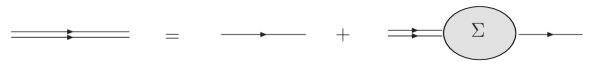
This fully dressed line should satisfy an equation analogous to the Dyson equation for the full propagator:

$$\widetilde{f}({\bf k})=f_{0}({\bf k})+sf_{0}({\bf k})\widetilde{f}({\bf k})\Sigma({\bf k}),$$ (60)

where $\Sigma({\bf k})$ is the sum of all (amputated) one-particle (1PI) insertions. Figure 5 represents this equation graphically.

Figure 5: Graphical representation of the integral equation (60). The double line represents $\widetilde{f}$, and the single line represents $f_{0}$.

Again we consider the analogy to Feynman diagrams. Take a two-particle irreducible (2PI) vacuum diagram with each internal line being fully dressed $\widetilde{f}$, and remove one internal line to form an amputated 1PI insertion. Summing over all ways of removing a line of a diagram, and then summing over all 2PI vacuum diagrams, the result is $\Sigma$.

Let $-\beta\digamma_{1}$ be the sum of all 2PI vacuum diagrams, with internal lines being $\widetilde{f}$ instead of $f_{0}$. The operations above can be neatly summarized by the following:

$$\Sigma({\bf k})=-s\beta\left({sf_{0}({\bf k})\over 1+sf_{0}({\bf k})}\right)^{-1}{\delta\,\digamma_{1}\over\delta f({\bf k})}.$$ (61)

The factor of $s$ is inserted by hand because the removal of one internal line decreases the loop count by one. One correctly surmises that $\digamma_{1}$ turns out to be the interaction part of $\digamma$. Indeed, when there is no interaction, all vertex functions are zero and $\digamma_{1}$ vanishes. The “Dyson” equation now reads:

$$\widetilde{f}({\bf k})-f_{0}({\bf k})+\beta\widetilde{f}({\bf k})(1+sf_{0}({\bf k})){\delta\digamma_{1}\over\delta f({\bf k})}=0.$$ (62)

and is actually an integral equation for $f$.

If we demand that the saddle point equation of the functional $\digamma$ leads to (62), then $\digamma_{0}$ can be uniquely fixed up to an additive constant and an overall scale. If we further demand that $\digamma_{0}$ reproduces the result of the free theory, then one can show that the only consistent choice is $\digamma=\digamma_{0}+\digamma_{1}$, where $\digamma_{0}$ is given in eq. (52) and

$$\digamma_{1}={\cal F}^{2PI}(f_{0}\to\widetilde{f})$$ (63)

i.e. $\digamma_{1}$ is given by the 2PI diagrams with $f_{0}$ replaced by the fully dressed $\widetilde{f}$. In Appendix A, we prove that the saddle point value of $\digamma$ is exactly ${\cal F}$, thus completing the derivation.

V Two-body aproximation

We shall now make the following approximations:

1. include only the four-vertex, i.e. ${\cal V}_{2}$, in our diagrammatic expansion;

2. consider only the foam diagrams, shown in Figure (6).

This should be the leading contribution in the low-density, high-temperature limit. When the density of the particles is low, we expect the two-particle scattering to be the most significant. At any given order of $f_{0}$, a foam diagram has the least number of vertices; since each vertex contributes a factor of $\beta$, the foam diagrams dominate in the limit of small $\beta$. In practice, this approximation amounts to setting

$$\digamma_{1}=-{1\over 2}\int(d{\bf k})(d{\bf k}^{\prime})\widetilde{f}({\bf k})\widetilde{f}({\bf k}^{\prime})G_{2}({\bf k},{\bf k}^{\prime}),$$ (64)

and truncating all terms with more $\widetilde{f}$.

Figure 6: Foam diagrams.

Within this approximation, the integral equation (62) can be rewritten into a self-consistent equation for the single-particle pseudo-energy. With the expressions (64) and (59), the equation (62) reduces to

$$\widetilde{f}({\bf k})=f_{0}({\bf k})+\widetilde{f}({\bf k})\left(s\beta f_{0}({\bf k})\int(d{\bf k}^{\prime})G_{2}({\bf k},{\bf k}^{\prime})\widetilde{f}({\bf k}^{\prime})\right).$$ (65)

In terms of the pseudo-energy $\epsilon_{\bf k}$ defined in eq. (57), using eq. (58) one can rewrite (65) as follows:

$$\epsilon_{{\bf k}}=\omega_{{\bf k}}-\mu-{1\over\beta}\log\left(1+\beta\int(d{\bf k}^{\prime})G_{2}({\bf k},{\bf k}^{\prime}){e^{\beta(\epsilon_{{\bf k}^{\prime}}-\omega_{{\bf k}^{\prime}}+\mu)}\over e^{\beta\epsilon_{{\bf k}^{\prime}}}-s}\right)$$ (66)

One may also want to find the free energy density of the system in terms of the physical filling fraction $f$. By using (65) and (56), it can be shown that

$$\digamma_{1} = -{1\over 2}\int(d{\bf k})(d{\bf k}^{\prime})\widetilde{f}({\bf k})\widetilde{f}({\bf k}^{\prime})G_{2}({\bf k},{\bf k}^{\prime})$$

$$= -{1\over 2\beta}\int(d{\bf k}){\widetilde{f}({\bf k})-f_{0}({\bf k})\over sf_{0}({\bf k})}$$

$$= -{1\over 2\beta}\int(d{\bf k}){f({\bf k})-f_{0}({\bf k})\over 1+sf_{0}({\bf k})}.$$

The free energy density then takes the simple form:

$${\cal F} = \digamma_{0}+\digamma_{1}$$

$$= -{1\over\beta}\int(d{\bf k})\left(s\log(1+sf)-{1\over 2}\left({f-f_{0}\over 1+sf_{0}}\right)\right)$$

In summary, the two-body approximation consists of the integral equation (66) for the pseudo-energy defined in eq. (57), and the above expression (V) for the free energy. The kernel that enters this approximation will be computed in the next section for Bose gases.

VI Two-body kernel for interacting Bose gases

VI.1 The kernel in arbitary dimensions.

The interacting Bose gas in $d$ spatial dimensions is defined by the hamiltonian

$$H=\int d^{d}{\bf x}\left({1\over 2m}|\vec{\nabla}\phi(x)|^{2}+{g\over 4}|\phi(x)|^{4}\right)$$ (69)

In this section, we derive the two-body kernel $G_{2}({\bf k}_{1},{\bf k}_{2})$ that enters the approximation of the last section. According to the definition in Section III, the kernel is the connected part of the diagonal matrix element of ${\rm Im}\log\widehat{S}(E)$. Since unitarity of $S$ implies it is a pure phase, one has

$$2\pi\delta\left(E-{1\over 2m}({\bf k}_{1}^{2}+{\bf k}_{2}^{2})\right)V\;G_{2}({\bf k}_{1},{\bf k}_{2})\equiv-i\langle{\bf k}_{1},{\bf k}_{2}|\log\widehat{S}(E)|{\bf k}_{1},{\bf k}_{2}\rangle.$$ (70)

where $V$ is the spatial volume. To define $\log(\widehat{S})$, we first follow the usual convention and write the two-body $S$-matrix as the sum of the identity operator and the $T$-matrix, as in eq. (19). The matrix elements of $\widehat{T}$ are the following:

$$\langle{\bf p}_{1},{\bf p}_{2}|\widehat{T}(E)|\mathbf{q}_{1},\mathbf{q}_{2}\rangle=(2\pi)^{d}\delta(\mathbf{p}_{1}+\mathbf{p}_{2}-\mathbf{q}_{1}-\mathbf{q}_{2})\widetilde{\mathcal{M}}_{q_{1},q_{2}\rightarrow p_{1},p_{2}}(E).$$ (71)

where $\widetilde{\mathcal{M}}_{q_{1},q_{2}\rightarrow p_{1},p_{2}}(E)$ denotes the two-body scattering amplitude from the in-state $|\mathbf{q}_{1},\mathbf{q}_{2}\rangle$ to the out-state $|\mathbf{p}_{1},\mathbf{p}_{2}\rangle$, assuming the energy $E$ of the in-state takes on some off-shell value. We’ll denote the on-shell version by $\mathcal{M}_{q_{1},q_{2}\rightarrow p_{1},p_{2}}$. Now $\log(\widehat{S})$ may be defined as a series of $\widehat{T}$:

$$\log(\widehat{S}(E))\equiv-\sum_{n=1}^{\infty}{(-1)^{n}\over n}\left[2\pi\delta(E-H_{0})\;i\,\widehat{T}(E)\right]^{n}.$$ (72)

The connectedness is guaranteed because, in terms of Feynman diagrams, $\widehat{T}$ does not contain any disconnected pieces.

The diagonal matrix elements of the $n$-th term of the above operator series,

$$\langle{\bf k}_{1},{\bf k}_{2}|\left[2\pi\delta(E-H_{0})\,i\,\widehat{T}(E)\right]^{n}|{\bf k}_{1},{\bf k}_{2}\rangle,$$

can be found by inserting copies of the resolution of the identity.

Note that the leftmost energy $\delta$-function hits the state $\langle{\bf k}_{1},{\bf k}_{2}|$, and consequently puts the energy $E$ on-shell. Moreover, given that the $S$-matrix is invariant under rotations and Galilean boosts, the on-shell amplitude $\mathcal{M}$ can only depend on the difference of the incoming momenta, which remains invariant due to conservation of energy and momentum. The amplitude $\mathcal{M}$ therefore remains constant throughout the entire available phase space, and can be taken out of any integration over the phase space. All put together, the diagonal matrix element of the $n$-th term of the series (72) is

$$\begin{split}\langle{\bf k}_{1},{\bf k}_{2}|\left[2\pi\delta(E-H_{0})\,i\,\widehat{T}(E)\right]^{n}|{\bf k}_{1},{\bf k}_{2}\rangle=&(2\pi)\delta\left(E-{1\over 2m}({\bf k}_{1}^{2}+{\bf k}_{2}^{2})\right)V\\ &\times\left(i\mathcal{M}(|{\bf k}_{1}-{\bf k}_{2}|)\right)^{n}\mathcal{I}^{n-1}.\end{split}$$ (73)

Here $\mathcal{I}=\mathcal{I}(|{\bf k}_{1}-{\bf k}_{2}|)$ is the volume of phase space available to the scattering out-state resulting from summing over all two-particle states in every intermediate resolution of identity:

$$\mathcal{I}(|{\bf k}_{1}-{\bf k}_{2}|)\equiv{1\over 2}\int(d{\bf p}_{1})(d{\bf p}_{2})(2\pi)^{d+1}\delta\left(E-{1\over 2m}({\bf p}_{1}^{2}+{\bf p}_{2}^{2})\right)\delta^{(d)}(\mathbf{P}-{\bf p}_{1}-{\bf p}_{2}),$$ (74)

where $E=({\bf k}_{1}^{2}+{\bf k}_{2}^{2})/2m$ and ${\bf P}={\bf k}_{1}+{\bf k}_{2}$ are the total energy and momentum of the in-state. Using this in (72), the resummation goes through trivially, and one obtains:

$$\langle{\bf k}_{1},{\bf k}_{2}|\log(\widehat{S}(E))|{\bf k}_{1},{\bf k}_{2}\rangle=2\pi\delta\left(E-{1\over 2m}({\bf k}_{1}^{2}+{\bf k}_{2}^{2})\right){V\over\mathcal{I}}\log\left(1+i\mathcal{I}\mathcal{M}(|{\bf k}_{1}-{\bf k}_{2}|)\right)$$ (75)

Finally, comparing this with (70), we have arrived at

$$G_{2}({\bf k}_{1},{\bf k}_{2})={-i\over\mathcal{I}}\log\left(1+i\mathcal{I}\,\mathcal{M}(|{\bf k}_{1}-{\bf k}_{2}|)\right).$$ (76)

Figure 7: Ladder diagram resummation of the two-body scattering amplitude.

The exact amplitude $\mathcal{M}$ in any number of dimensions $d$ can be calculated by resumming ladder diagrams (Fig 7):

$$\begin{split}i\mathcal{M}&=(-ig)+\dfrac{1}{2}(-ig)^{2}\int(\text{loop})+\dfrac{1}{4}(-ig)^{3}\left(\int(\text{loop})\right)^{2}+\dots\\ &=-ig\left(1+{ig\over 2}\int(\text{loop})\right)^{-1}\end{split}$$ (77)

where the loop integral is

$$\int(\text{loop})=\int(d\omega)(d{\bf k})\left({i\over\omega-k^{2}/2m+i\epsilon}\right)\;\left({i\over(E-\omega)-(\mathbf{P}-{\bf k})^{2}/2m+i\epsilon}\right)$$ (78)

VI.2 The kernel in two dimensions.

The first step of the calculation is to compute the kernel by setting $d=2$ in equations (76), (74) and (77). In dimension $d=2$ the phase space volume $\mathcal{I}=m/4$.

The loop integral diverges in $d=2$, and must be regularized with a UV momentum cutoff $\Lambda$. The final form of $\mathcal{M}$ is:

$$\mathcal{M}(|{\bf k}_{1}-{\bf k}_{2}|)=-{g\over 1+{mg\over 8\pi}\left(\log\left({4\Lambda^{2}\over|{\bf k}_{1}-{\bf k}_{2}|^{2}}\right)+i\pi\right)}$$ (79)

When all put together, the kernel $G_{2}$ is the following:

$$\begin{split}G_{2}({\bf k}_{1},{\bf k}_{2})&={-4i\over m}\log\left({1+{mg\over 8\pi}\left(\log\left({4\Lambda^{2}\over|{\bf k}_{1}-{\bf k}_{2}|^{2}}\right)-i\pi\right)\over 1+{mg\over 8\pi}\left(\log\left({4\Lambda^{2}\over|{\bf k}_{1}-{\bf k}_{2}|^{2}}\right)+i\pi\right)}\right)\\ &=-\dfrac{8}{m}\arctan\left({mg/8\over 1+{mg\over 8\pi}\log\left({4\Lambda^{2}\over|{\bf k}_{1}-{\bf k}_{2}|^{2}}\right)}\right)\end{split}$$ (80)

VI.3 The kernel in three dimensions

Computation of the two-body kernel in $d=3$ has little different from the 2-dimensional case. The phase space volume (74) turns out to be:

$$\mathcal{I}={m\over 8\pi}|{\bf k}_{1}-{\bf k}_{2}|.$$ (81)

Once again the loop integral is UV divergent and in principle needs a cutoff $\Lambda$. The divergence is linear in $\Lambda$, and can be completely absorbed by a redefinition of the coupling constant. We proceed to define the renormalized coupling $g_{R}$ by

$${1\over g_{R}}={1\over g}+{m\Lambda\over 4\pi^{2}}.$$ (82)

The amplitude (77) becomes

$$i\mathcal{M}={-ig_{R}\over 1+i{mg_{R}\over 16\pi}|{\bf k}_{1}-{\bf k}_{2}|}.$$ (83)

The two-body kernel (76) is then

$$\begin{split}G_{2}({\bf k}_{1},{\bf k}_{2})&=-i{8\pi\over m|{\bf k}_{1}-{\bf k}_{2}|}\log\left({1-{img_{R}\over 16\pi}|{\bf k}_{1}-{\bf k}_{2}|\over 1+{img_{R}\over 16\pi}|{\bf k}_{1}-{\bf k}_{2}|}\right)\\ &=-{16\pi\over m|{\bf k}_{1}-{\bf k}_{2}|}\arctan\left({mg_{R}\over 16\pi}|{\bf k}_{1}-{\bf k}_{2}|\right)\end{split}$$ (84)

VII One-dimensional case: comparison with the thermodynamic Bethe ansatz.

In one spatial dimension, the thermodynamic Bethe ansatz (TBA) is applicable if the model is integrable, leading to an exact expression for the free energy. As explained in the Introduction, our formalism is modeled after the TBA, and is constructed from the same ingredients: the filling fractions and free energy are expressed in terms of a pseudo-energy $\epsilon(k)$, and the latter satisfies an integral equation based on the exact S-matrix. If the model is integrable, the n-body S-matrix factorizes into 2-body S-matrices, and the TBA incorporates these n-body interactions in its derivation and the final result is expressed only in terms of the 2-body S-matrix. The TBA thus goes beyond the 2-body approximation described in section V. Nevertheless, our formalism should coincide with the TBA to lowest order in the scattering kernel, and in this section we show this is indeed the case.

VII.1 Kernel

In this section, we shall specialize in the case $d=1$. Also, we shall set $m=1/2$ throughout this section. The on-shell value of energy for the two-particle in-state $|k_{1},k_{2}\rangle$ is $E=k_{1}^{2}+k_{2}^{2}$. With this identification, the phase space volume (74) turns out to be

$$\mathcal{I}={1\over 2|k_{1}-k_{2}|}$$ (85)

The two-body amplitude (77) in $d=1$ is

$$i\mathcal{M}={-ig\over 1+{ig\over 4(k_{1}-k_{2})}}.$$ (86)

The kernel (76) then becomes:

$$G_{2}(k_{1},k_{2})=-2i(k_{1}-k_{2})\log\left({(k_{1}-k_{2})-ig/4\over(k_{1}-k_{2})+ig/4}\right).$$ (87)

VII.2 Comparision with TBA

In one spatial dimenion, the interacting boson with hamiltonian (69) is known to be exactly solvable using the TBA. In particular, the free energy is

$${\cal F}=-{1\over\beta}\int(dk)\log\left(1+e^{-\beta\epsilon(k)}\right),$$ (88)

where $\epsilon(k)$ obeys the Yang-Yang equation:

$$\epsilon(k)=k^{2}-{1\over\beta}\int(dk^{\prime})K(k,k^{\prime})\log(1+e^{-\beta\epsilon(k^{\prime})}),$$ (89)

The TBA kernel $K$ is the derivative of the $\log$ of the S-matrix

$$S(k,k^{\prime})={k-k^{\prime}-ig/4\over k-k^{\prime}+ig/4}$$ (90)

$$K(k,k^{\prime})=-i\partial_{k}\log S(k,k^{\prime})={g/2\over(k-k^{\prime})^{2}+(g/4)^{2}}.$$ (91)

Comparing with (33), one sees that the signs in (88) are fermionic. The TBA is really a description of the model in terms of its fermionic dual.

Expanding the right hand side of (88) to the leading order in the kernel $K$ using (89), we have

$${\cal F}\approx{\cal F}_{0}+\int(dk)f_{0}(k)\left[-{1\over\beta}\int(dk^{\prime})K(k,k^{\prime})\log\left(1+e^{-\beta\omega_{k^{\prime}}}\right)\right]$$ (92)

Integrating the right hand side by parts with respect to $k^{\prime}$ one obtains

$${\cal F}\approx{\cal F}_{0}-{1\over 2}\int(dk)(dk^{\prime})f_{0}(k)f_{0}(k^{\prime})\left(-2i|k-k^{\prime}|\log\left({(k-k^{\prime})-ig/4\over(k-k^{\prime})+ig/4}\right)\right)$$ (93)

The above expression coincides with the $N=1$ term of (44), the first order correction of our formulation, with the kernel $G_{2}(k,k^{\prime})$ given by (87).

VIII Acknowledgments

We would like to thank Erich Mueller for discussions. This work is supported by the National Science Foundation under grant number NSF-PHY-0757868.

IX Appendix A

We shall now show that the saddle point value of $\digamma$ as defined in (53) equals the free energy ${\cal F}$ given in (37). Throughout this section the integral equation (62) is always assumed to be satisfied.

First, let us define

$$\Delta f({\bf k})\equiv\widetilde{f}({\bf k})-f_{0}({\bf k}),$$ (94)

i.e. $\Delta f$ is the sum of all digrams with two external legs and any non-trivial insertion. In particular, the sum is not restricted to 2PI terms only; all one-particle reducible terms are also included. By re-arranging (56), we get one useful identity:

$${\Delta f\over f_{0}}={s(f-f_{0})\over 1+sf_{0}}$$ (95)

We will now rewrite $\digamma_{0}$ in a more convenient form using (95):

$$\digamma_{0} \equiv -{1\over\beta}\int(d{\bf k})\left(s\log(1+sf)-\left({f-f_{0}\over 1+sf_{0}}\right)\right)$$

$$= -{1\over\beta}\int(d{\bf k})\left[s\log(1+sf_{0})+s\log\left(1+{\Delta f\over f_{0}}\right)-s{\Delta f\over f_{0}}\right]$$

$$= {\cal F}_{0}+{1\over\beta}\int(d{\bf k})\,s\sum_{n=2}^{\infty}{1\over n}\left({-\Delta f\over f_{0}}\right)^{n}$$

As for the using interaction part of $\digamma$, one can show using the integral equation (62):

$$\digamma_{1} \equiv -{1\over 2\beta}\int(d{\bf k})(d{\bf k}^{\prime})\,\widetilde{f}({\bf k})\widetilde{f}({\bf k}^{\prime})w_{2}({\bf k},{\bf k}^{\prime})$$

$$= -{s\over 2\beta}\int(d{\bf k}){\Delta f({\bf k})\over f_{0}({\bf k})}.$$

Together we conclude that the saddle point value of $\digamma$ is

$$\digamma={\cal F}_{0}+{s\over\beta}\int(d{\bf k})\,\left[-{1\over 2}{\Delta f\over f_{0}}+\sum_{n=2}^{\infty}{1\over n}\left(-{\Delta f\over f_{0}}\right)^{n}\right]$$ (98)

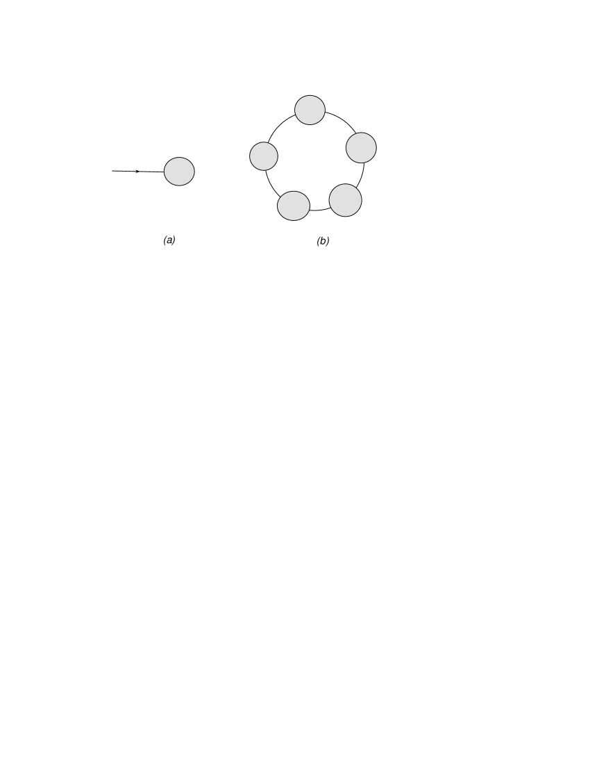
We shall now give this equation a graphical meaning. Recall that $\Delta f$ represents the sum of all diagrams with two external legs and some non-trivial structure between the two legs. $\Delta f/f_{0}$ is then the sum of such diagrams with one of the two legs amputated. The quantity $s\int(d{\bf k})(\Delta f(k)/f_{0}(k))^{n}$ then represents a ring with $n$ non-trivial insertions, with the factor of $s$ again coming from the loop. (See Figure 8) Again we stress that such insertion needs not be 1PI.

Figure 8: (a) Graphical representation of $\Delta f/f_{0}$; one of the two external legs is amputated. (b) The graph for $s\int(d{\bf k})(\Delta f(k)/f_{0}(k))^{n}$. In this example $n=5$.

The correction to the free energy $\digamma-{\cal F}_{0}$ can then be graphically represented as Figure 9. The factor $1/n$ of the $n$th order term in (98) is cancelled because there are $n$ ways to order these $n$ insertions to form an identical ring, not counting possible extra symmetry.

Figure 9: Graphical representation of $\digamma-{\cal F}_{0}$.

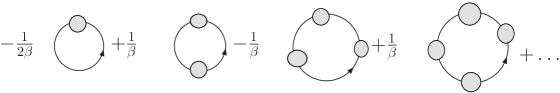
Recall that, within the foam-diagram approximation, the free energy (37) is really ${\cal F}_{0}$ plus the sum of all connected foam diagrams. Every term in Figure 9 is a foam diagram by construction. To prove the equality of (37) and (98), we only need to verify (98), or equivalently Figure 9, produce the correct coefficient for every foam diagram.

Consider a foam diagram with $N$ loops labeled $i=1\dots N$, and the $i$th loop has $n_{i}$ vertices attached to it. It can be shown that

$$\sum_{i=1}^{N}n_{i}=2N-2.$$ (99)

Now we consider how the particular foam diagram may be constructed from Figure 9 if the loops shown is the $i$th loop of the diagram. The $i$-th loop has $n_{i}$ vertices; it can be built from terms with at most $n_{i}$ insertions. The $m$-th order term contributes only if $m\leq n_{i}$. The number of ways to partition the $n_{i}$ 1PI insertions into $m$ connected groups is simply the binomial coefficient $C^{m}_{n_{i}}$.

We can now sum over every loop of the diagram to get the overall coeficient:

$$\sum_{i=1}^{N}\left[{1\over 2}C^{1}_{n_{i}}-\sum_{m=2}^{n_{i}}(-1)^{m}C^{m}_{n_{i}}\right] = \sum_{i=1}^{N}\left[-\sum_{m=0}^{n_{i}}(-1)^{m}C^{m}_{n_{i}}-{1\over 2}C^{1}_{n_{i}}+C^{0}_{n_{i}}\right]$$

$$= \sum_{i=1}^{N}\left[-(1-1)^{n_{i}}-{1\over 2}n_{i}+1\right]$$

$$= 1$$

We have used the identity (99) to evaluate the sum. This shows that the coefficient of a diagram without symmetry equals exactly unity. If a diagram has an $N$-fold rotational symmetry, then the above counting argument overcounts the contribution by $N$ times, and a symmetry factor $1/N$ is needed.

We have thus proven that $\digamma_{1}$ in eq. (IX) generates every foam diagram with the correct coefficient. Its saddle point value is therefore the correct free energy of the system within the foam-diagram approximation.

References

- (1) V. N. Popov, Functional Integrals in Quantum Field Theory and Statistical Physics, (Reidel, Dordrecht, 1983).
- (2) D. S. Fisher and P. C. Hohenberg, Phys. Rev. B37 (1988) 4936.
- (3) M. Holzmann, G. Baym, J.-P. Blaizot and F. Laloë, Proc. Natl. Acad. Sci. USA 104 (2007) 1476, arXiv:cond-mat/0508131.
- (4) N. Prokof’ev, O. Ruebenacker and B. Svistunov, Phys. Rev. Lett. 87 (2001) 270402.
- (5) A. Posazhennikova, Rev. Mod. Phys. 78 (2006) 1111.
- (6) P. Krüger, Z. Hadzibabic and J. Dalibard, Phys. Rev. Lett. 99 (2007) 040402.
- (7) E. Lieb and W. Liniger, Phys. Rev. 130 (1963) 1605.
- (8) C. N. Yang and C. P. Yang, Jour. Math. Phys. 10, (1969) 1115.
- (9) R. Dashen, S.-K. Ma and H. J. Bernstein, Phys. Rev. 187 (1969) 345.
- (10) A. LeClair, J. Phys. A40 (2007) 9655; Int. J. Mod. Phys. A23 (2008) 1371.
- (11) T. D. Lee and C. N. Yang, Phys. Rev. 113 (1959) 1165; Phys. Rev. 117 (1960) 22.