A Compton-thick Wind in the High Luminosity Quasar, PDS 456.

Abstract

PDS 456 is a nearby (z=0.184), luminous ($L_{\rm bol}\sim 10^{47}$ erg s^-1) type I quasar. A deep 190 ks Suzaku observation in February 2007 revealed the complex, broad band X-ray spectrum of PDS 456. The Suzaku spectrum exhibits highly statistically significant absorption features near 9 keV in the quasar rest–frame. We show that the most plausible origin of the absorption is from blue-shifted resonance ($1s-2p$) transitions of hydrogen-like iron (at 6.97 keV in the rest frame). This indicates that a highly ionized outflow may be present moving at near relativistic velocities ($\sim 0.25c$). A possible hard X-ray excess is detected above 15 keV with HXD (at 99.8% confidence), which may arise from high column density gas ($N_{\rm H}>10^{24}$ cm^-2) partially covering the X-ray emission, or through strong Compton reflection. Here we propose that the iron K-shell absorption in PDS 456 is associated with a thick, possibly clumpy outflow, covering about 20% of $4\pi$ steradian solid angle. The outflow is likely launched from the inner accretion disk, within 15–100 gravitational radii of the black hole. The kinetic power of the outflow may be similar to the bolometric luminosity of PDS 456. Such a powerful wind could have a significant effect on the co-evolution of the host galaxy and its supermassive black hole, through feedback.

1 Introduction

Outflows are an important phenomenon in AGN and may play a key role in the co-evolution of the massive black hole and the host galaxy. Black holes grow by accretion and strong nuclear outflows can quench this process by effectively shutting off the supply of matter. At high redshifts, such quasar winds could have provided crucial feedback that controlled both the formation of stellar bulges and simultaneously self-regulated SMBH growth, leading ultimately to the observed $M$–$\sigma$ relation for galaxies (Ferrarese & Merritt, 2000; Gebhardt et al., 2000). A wind, launched within a few gravitational radii of the black hole, can move into the host galaxy, pushing material outwards until, at a critical black hole mass, the ISM is effectively evacuated, quenching star formation and stopping further SMBH growth. Thus accretion disk outflows may help regulate the growth of the galactic bulge and the central black hole in galaxies (Silk & Rees, 1998; Fabian, 1999; King, 2003; Di Matteo et al., 2005).

Recently a number of high column density ($N_{\rm H}\sim 10^{23}-10^{24}$ cm^-2), fast ($>0.1c$) outflows have been claimed in several AGN (Chartas et al., 2002, 2003; Hasinger et al., 2002; Reeves et al., 2003; Pounds et al., 2003; Dadina et al., 2005; Gibson et al., 2005; Markowitz et al., 2006; Braito et al., 2007; Papadakis et al., 2007), through detections of blue-shifted K-shell absorption lines of iron, observed at rest-frame energies greater than 7 keV. These fast outflows are likely driven off the accretion disk by either radiation pressure (Proga et al., 2000; Proga & Kallman, 2004; Sim et al., 2008) or magneto-rotational forces (Kato et al., 2004), or both, a few gravitational radii from the black hole. In some cases the outflow rates derived can be huge, of several solar masses per year, equivalent to $10^{45}-10^{46}$ erg s^-1 in kinetic power (Reeves et al., 2003; Pounds et al., 2003), matching the radiative luminosity of the AGN and can have a significant effect on the host galaxy evolution (King, 2003). Such outflows are a likely consequence of near-Eddington accretion (King & Pounds, 2003) and are key to understanding accretion at high Eddington rates.

Here we present a deep 2007 Suzaku observation of the nearby ($z=0.184$, Torres et al. (1997)) and luminous ($L_{\rm bol}\sim 10^{47}$ erg s^-1, Simpson et al. (1999); Reeves et al. (2000)) type I quasar PDS 456. A previous 40 ks XMM-Newton observation revealed the presence of deep iron K-shell absorption above 7 keV, which may be attributed to a high column density outflow (Reeves et al., 2003), while PDS 456 also exhibits blue-shifted absorption in the UV (O’Brien et al., 2005). An analysis of the Suzaku XIS data reveals direct evidence for blue-shifted absorption lines in the iron K-shell band (see Sections 3 and 4), which may arise from a near relativistic outflow, launched from the inner quasar accretion disk. We also report on a tentative detection of hard X-ray emission above 15 keV in the Suzaku HXD observation of PDS 456. Values of H₀=70 km s^-1 Mpc^-1, and $\Omega_{\Lambda_{\rm 0}}=0.73$ are assumed throughout and errors are quoted at 90% confidence ($\Delta\chi^{2}=2.7$), for 1 parameter of interest.

2 Suzaku Observations of PDS 456

PDS 456 was observed by Suzaku (Mitsuda et al., 2007) at the XIS nominal pointing position between 24 Feb to 1 Mar 2007 (sequence number 701056010), over a total duration of 370 ks. A summary of observations is shown in Table 1. Data were analysed from the X-ray Imaging Spectrometer XIS (Koyama et al., 2007) and the PIN diodes of the Hard X-ray Detector HXD/PIN (Takahashi et al., 2007) and processed using v2 of the Suzaku pipeline. Data were excluded within 436 seconds of passage through the South Atlantic Anomaly (SAA) and within Earth elevation angles or Bright Earth angles of $<5^{\circ}$ and $<20^{\circ}$ respectively.

2.1 XIS analysis

XIS data were selected in $3\times 3$ and $5\times 5$ editmodes using grades 0,2,3,4,6, while hot and flickering pixels were removed using the sisclean script. Spectra were extracted from within circular regions of 2.9′ diameter, while background spectra were extracted from 4 circles offset from the source and avoiding the chip corners containing the calibration sources. The response matrix (rmf) and ancillary response (arfs) files were created using the tasks xisrmfgen and xissimarfgen, respectively, the former accounting for the CCD charge injection and the latter for the hydrocarbon contamination on the optical blocking filter. Spectra from the two front illuminated XIS 0 and XIS 3 chips were combined to create a single source spectrum (hereafter XIS–FI), while data from the back illuminated XIS 1 chip were analysed separately. Data were included from 0.45–10 keV for the XIS–FI and 0.45–7 keV for the XIS 1 chip, the latter being optimized for the soft X-ray band. The net background subtracted source count rates were $0.521\pm 0.002$ cts s^-1 for XIS–FI and $0.413\pm 0.002$ cts s^-1 for XIS 1, with a net exposure of 179.7 ks. XIS background rates correspond to only 1.5% and 3.3% of the net source counts for XIS–FI and XIS 1 respectively. The XIS spectra were subsequently binned to a minimum energy width corresponding to approximately the $1\sigma$ XIS resolution of 60 eV at 6 keV, dropping to 30 eV at lower energies. Channels were additionally grouped to achieve a minimum S/N of 5 per bin over the background and $\chi^{2}$ minimization was used for all subsequent spectral fitting.

2.2 HXD analysis

The Suzaku HXD/PIN is a non-imaging instrument with a 34′ square (FWHM) field of view. For weak hard X-ray sources (i.e. many AGN) where the source count rate is only a few percent of the background rate, it is crucial to correctly subtract the variable non X-ray background (i.e. the particle or detector background) to obtain an accurate estimate of the net source count rate. The HXD instrument team provide two Non X-ray Background (NXB) events files for this purpose; the background–A model (also known as the “quick” background) and the background–D model (or “tuned” background). The systematic uncertainty of the background–D model is believed to be lower than for background–A, typically $\pm 1.3$% at the $1\sigma$ level for a net 20 ks exposure (Fukazawa et al., 2009).

To determine which model provides the most reliable estimate of the background, the background–A or D lightcurve was compared to the lightcurve obtained from the Earth occulted data (from Earth elevation angles ${\rm ELV}<-5$), in the 15–50 keV band. The Earth occulted data gives a representation of the actual NXB rate, as this neither includes a contribution from the source nor from the Cosmic X-ray background (CXB). The Earth occulted data were corrected for deadtime, using the pseudo events file. Figure 1 (top and middle panels) shows the comparison for each of the background models with the Earth rate. Specifically, we calculated the ratio (Earth $-$ bgd [A or D]) / bgd [A or D]; i.e. the difference between the Earth and background model rates normalized to the background model rate. The lightcurves are heavily binned (15 satellite orbits or 86.4 ks) in order to increase signal to noise. For the background–A model, the model clearly underpredicts the Earth background rate, by $+8.8\pm 1.0$%. In contrast for background–D, the model slightly overpredicts the Earth rate, by the ratio $-2.4\pm 1.0$%. Thus subsequently we adopt the background D model as the likely more accurate background model, noting that for this observation it slightly overpredicts the Earth background rate, by 2.4%, which we correct for in the subsequent analysis.

The background–D NXB events file was then used in conjunction with the screened source events file (from rev2 of the pipeline processing) to create a common good time interval. The files were thus used to calculate lightcurves (binned into 5 orbital bins or 28.8 ks) for both the source (deadtime corrected) and for the detector (NXB) background; note a $1\sigma$ systematic error of $\pm 1.3$% was included in the NXB rate. Figure 1 (lower panel) shows the PIN source lightcurve (after subtraction of the NXB) from 15–50 keV. The expected contribution from the diffuse (non-variable) Cosmic X-ray Background (CXB), using the spectral form of Gruber et al. (1999), was also calculated; in the 15–50 keV band this is expected to contribute 0.017 cts s^-1 to the total count rate (or a 15-50 keV flux of $7.9\times 10^{-12}$ erg cm^-2 s^-1). We include a $\pm 10$% uncertainty in the absolute normalization of the CXB. Note a more detailed discussion of the CXB and possible contamination in the HXD field of view is given in Appendix A.

Thus the mean net source count rate, after subtraction of both the NXB and CXB components (i.e. total background = NXB + CXB), is $(1.5\pm 0.3)\times 10^{-2}$ counts s^-1, and is about 5% of the total background count rate (0.33 counts s^-1). This corresponds to a source flux of $(7.3\pm 2.4)\times 10^{-12}$ erg cm^-2 s^-1 (including 1.3% systematic uncertainty on the background) from 15-50 keV, assuming a power-law photon index of $\Gamma=2$. In comparison the source flux derived from using background–A is higher, $(1.2\pm 0.3)\times 10^{-11}$ erg cm^-2 s^-1 from $15-50$ keV; hereafter we adopt the more conservative flux derived from background–D. This represents the first possible detection of PDS 456 in the hard X-ray band above 15 keV, at the significance level of $7\sigma$ (statistical) or $\sim 3\sigma$ (statistical+systematic) above the background and is below the expected sensitivity level of the Swift-BAT all sky survey, of about $10^{-11}$ erg cm^-2 s^-1 (Tueller et al., 2008).

A net (deadtime-corrected) source spectrum was subsequently extracted in the 15-50 keV range (subtracting both the NXB and CXB) which yielded a net PIN exposure of 164.8 ks and the same net count rate as above from 15-50 keV. The deadtime rate for the source events was 6.7%. The response file ae-hxd-pinxinome3-20080129.rsp provided by the instrument team was used in all the spectral fits below. The HXD/PIN spectrum was initially binned to a single bin, to represent a flux point between 15-50 keV, as described above. A finer binning of $2\sigma$ per bin above the background was subsequently used for the spectral fits in sections 4 and 5. Note that a cross-normalization factor of 1.16 is included between the HXD/PIN and XIS, as calculated for observations of the Crab.

3 Detection of the Iron K-shell Absorber

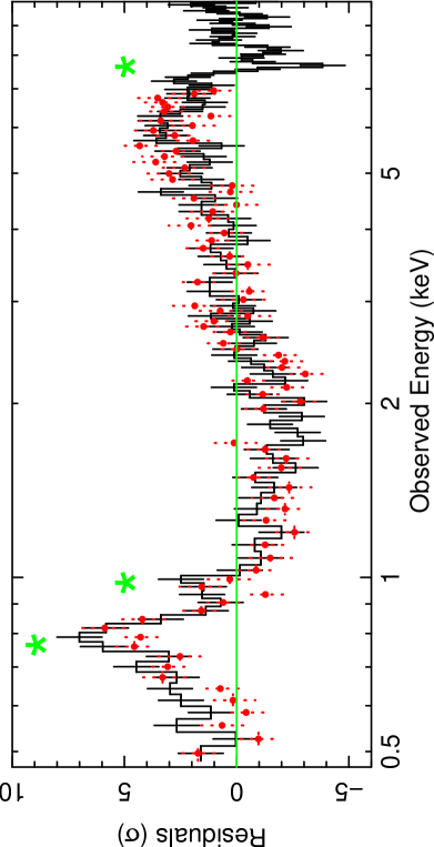
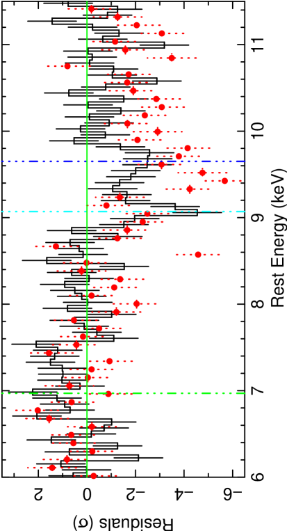
Figure 2: Upper panel - Suzaku XIS spectra of PDS 456, plotted as a ratio to a simple absorbed power-law ($\Gamma=2.2$). Note XIS 1 is shown in red, XIS–FI in black. The position of the two soft X-ray emission lines and of the Fe K-shell absorption are marked with a star. Lower panel - rest frame iron K-shell absorption in PDS 456 (against the best fit, broken power-law continuum). Suzaku XIS–FI is shown in black, XMM-Newton EPIC-pn (2001) in red. The green line represents the expected position of the Fe xxvi $1s-2p$ line (6.97 keV), while the blue lines represent the centroids of the detected absorption lines in XIS.

Initially we consider the X-ray spectrum of PDS 456 in the 0.45–10 keV band using the XIS alone. Galactic absorption of $2\times 10^{21}$ cm^-2 (Dickey & Lockman, 1990; Kalberla et al., 2005) was adopted, modeled with the “Tuebingen–Boulder” absorption model (tbabs in xspec) using the cross–sections and abundances of Wilms et al. (2000). Figure 2 (upper panel) shows the residuals to the XIS spectra to a single power-law of $\Gamma=2.35\pm 0.01$ with Galactic absorption. Evidently this is a poor fit (fit statistic, $\chi^{2}/{\rm dof}=1004.4/391$); the 0.45–10 keV spectrum is concave, steepening towards lower energies, while there appears to be strong soft X-ray line emission observed near 0.75–0.80 keV and absorption at higher energies above 7.5 keV.

We thus proceed to parameterize the XIS continuum with a broken power-law with $\Gamma_{\rm soft}=2.44\pm 0.04$, a break at $E=2.0\pm 0.2$ keV and $\Gamma_{\rm hard}=2.24\pm 0.02$ towards higher energies. Soft X-ray line emission is required, with one strong and broadened line at $E=0.91\pm 0.01$ keV (QSO rest–frame) with an equivalent width of ${\rm EW}=42\pm 10$ eV, intrinsic width of $\sigma=75\pm 15$ eV (FWHM 57000 km s^-1) and a weak narrow line at $E=1.16\pm 0.02$ keV with ${\rm EW}=6\pm 3$ eV. Note a summary of the spectral fit parameters is shown in Table 2. The former line may be associated with either the Ne ix triplet (0.909–0.921 keV), L-shell ($3d-2p$) emission from Fe xix (at 0.92 keV) or a blend of the two, the latter may be identified with Fe xxiv L-shell (1.16 keV).

The fit statistic is still poor ($\chi^{2}/{\rm dof}=529.3/382$, null hypothesis probability of $8.3\times 10^{-7}$) and is significantly improved by the addition of two blue-shifted absorption lines observed at $7.67\pm 0.04$ keV and $8.13\pm 0.07$ keV (or at $9.09\pm 0.05$ keV and $9.64\pm 0.08$ keV in the quasar rest-frame). The fit is improved by $\Delta\chi^{2}=41.1$ upon first adding the lower energy line and further by an additional $\Delta\chi^{2}=29.0$ upon adding the 2nd higher energy line to the model. In total the fit improves by $\Delta\chi^{2}=70$ upon adding both lines to the model.

The line EWs are high at $-133\pm 39$ eV and $-129\pm 48$ eV respectively. The intrinsic width of the absorption lines is marginally resolved $\sigma=105^{+55}_{-65}$ eV, after subtracting the instrumental resolution of $\sigma=60$ eV at Fe K. Thus the FWHM velocity is loosely constrained to be $8000^{+4000}_{-5000}$ km s^-1. Note the width of the lines are tied to have the same value as each other.

The possibility that the absorption arises from a single, but broader line was also investigated. We note that although this cannot be firmly ruled out, the resulting fit is slightly worse ($\Delta\chi^{2}=12$ for 1 parameter) than for the fit with 2 absorption lines, while the line width is substantially broadened ($\sigma=0.40\pm 0.12$ keV or a FWHM of $\sim 30000$ km s^-1).

There is also evidence for broadened ionized iron K$\alpha$ emission at $7.2\pm 0.2$ keV in the quasar rest-frame (${\rm EW}=132\pm 52$ eV, $\sigma=0.35^{+0.65}_{-0.14}$ keV or $\sim 30000$ km s^-1 (FWHM), $\Delta\chi^{2}=27.7$). The final fit statistic is then $\chi^{2}/{\rm dof}=431.5/374$. We will return to the origin of the iron K and L-shell emission in Section 5.

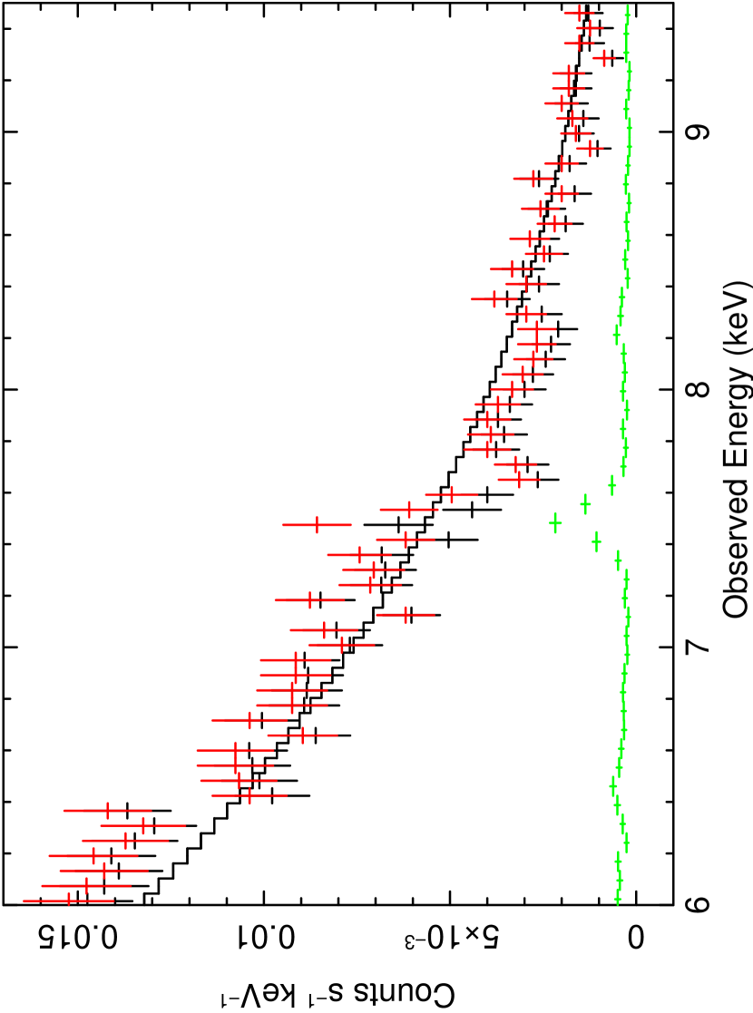
Figure 3: Suzaku XIS–FI PDS 456 spectrum versus the background spectrum in the iron K band. The source spectrum prior to background subtraction in shown in red, the net source spectrum after background subtraction is in black and the background spectrum is in green. The black line shows the broken powerlaw continuum model, folded through the XIS response. It can be seen that the background subtraction has little effect in the iron K band and on the absorption features at 7.7 keV and 8.2 keV (observed frame). Overall the level of the XIS background is low and the only strong background line arises from Ni K$\alpha$ at 7.45 keV, which is not coincident with the centroids of the absorption lines from PDS 456. Note the normalization of the background has been rescaled to that of the XIS source region size.

We note that the absorption line detections are robust against the detector background of the XIS–FI CCDs, which is $<2$% of the net source count rate, while the strongest emission line in the background spectrum (Ni i K$\alpha$ at 7.47 keV) does not coincide with either of the absorption lines (note that unlike in XMM-Newton EPIC-pn spectra, no Cu K$\alpha$ line is present in Suzaku XIS background spectra at 8 keV). The comparison between the net source spectrum and background spectrum is plotted in Figure 3.

3.1 Statistical Significance of the Absorption Lines

The significance of the iron K absorption lines was estimated using multi–trial Monte Carlo simulations. The method used was identical to that described in Porquet et al. (2004) and Markowitz et al. (2006). Specifically we generated 3000 random XIS-FI spectra with an initial input continuum, exposure and background as per the actual PDS 456 data, but under the null hypothesis of no absorption lines. The spectra were stepped in energy increments of 30 eV over the 0.6–9 keV energy band, i.e. where any absorption lines may be reasonably expected to be found, in order to map the distribution of $\Delta\chi^{2}$ for the trials. We ignore data below 0.6 keV as this may be effected by the calibration around the detector O edge and above 9 keV (observed) where the XIS effective area drops rapidly.

In the actual data, two absorption lines were found, yielding improvements to the fit statistic of $\Delta\chi^{2}=41.1$ and 29.0 respectively. In the simulated spectra, these values correspond to 1 and 3 out of the 3000 spectra respectively. Thus the null hypothesis probability that each of the individual lines is due to random statistical fluctuation is $3\times 10^{-4}$ and $1\times 10^{-3}$ respectively (i.e. $3.6\sigma$ and $3.2\sigma$). Indeed this significance is likely to be highly conservative, as the probablity was estimated from a blind search over 3000 random spectra and stepping through 280 energy increments (of 30 eV) in each spectrum.

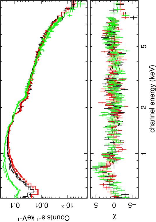
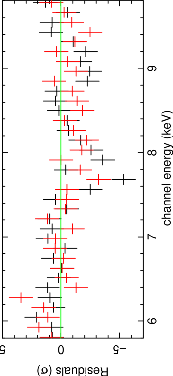
Figure 4: XIS 0 (black), XIS 1 (green) and XIS 3 (red) spectra of PDS 456, compared to the baseline broken power-law continuum model. The top panel shows the data folded through the instrumental response, the lower panel the residuals compared to the continuum. Here the data is binned with a minimum S/N of 10 for XIS 0, 3 and S/N of 5 for XIS 1. Note the excess soft X-ray emission (0.8 keV observed) and hard X-ray absorption (7.5–8.0 keV) is present in all 3 XIS detectors. The lower panel show the comparison between XIS 0 and 3 in the Fe K band, where the iron K absorption is observed, with the data binned at the instrumental (FWHM) resolution.

We further note that the 9 keV rest-frame absorption is also independently detected in both XIS–FI CCDs, XIS 0 and XIS 3, although the detection is marginal in the back-illuminated XIS 1 which has little sensitivity above 7 keV. Figure 4 (top, middle) shows the XIS 0, 1, 3 spectra compared to the best fit broken power-law continuum, which shows the spectra from all 3 XIS are consistent within the statistical errors. Figure 4 (lower panel) also shows a comparison of the XIS 0 and 3 in the Fe K band, which illustrates the independent detection of the Fe K absorption in both the XIS FI CCD’s. The absorption line parameters are consistent between XIS 0 and 3; for XIS 0 the first line has an rest-frame energy $E=9.06\pm 0.05$ keV and $EW=-164\pm 47$ eV and the second line $E=9.47\pm 0.05$ keV and $EW=-149\pm 60$ eV, for XIS 3 these values are $E=9.12\pm 0.09$ keV, $EW=-113\pm 52$ eV and $E=9.62\pm 0.15$ keV, $EW=-101\pm 64$ eV respectively. The upper-limits obtained from XIS 1 are consistent with these values.

We also performed Monte Carlo simulations on 3000 spectra for XIS 0 and 3 indepedently, as the line appears consistent in both detectors. As these are totally independent measurements, the resulting null probabilities are the product of the probabilities for XIS 0 and 3 seperately, which are then $1.2\times 10^{-5}$ ($4.4\sigma$) for the lower energy line and $4.2\times 10^{-3}$ ($2.9\sigma$) for the higher energy line.

The likelihood that the absorption is due to random chance is also further diminished when the 2001 XMM-Newton data are considered. Figure 2 (lower panel) also plots the 2001 EPIC-pn data overlaid upon the Suzaku XIS spectrum. Absorption is clearly present in the XMM-Newton data (with a trough apparent between 9–10 keV, quasar rest frame), although the exact absorption profile may have varied. Indeed the possibility of deep iron K absorption in PDS 456 was first noted in Reeves et al. (2000), on the basis of low resolution RXTE PCA data and also with Beepo-SAX MECS (Vignali et al. 2000). Thus the coincidence of absorption in two independent detectors (XIS 0, 3) and telescopes (Suzaku, XMM-Newton) at very similar energies would appear to confirm the detection of the blue-shifted absorption in PDS 456.

4 The Origin of the Iron band Absorption

The possible origin of the iron K band absorption is now discussed.

4.1 Identification of the Absorption Lines

As shown above, the absorption lines detected in the XIS appear to be highly blue-shifted with respect to the iron K-shell band, with QSO rest–frame energies of $9.09\pm 0.05$ keV and $9.64\pm 0.08$ keV. Figure 2 (lower panel) shows the XIS–FI residuals in the iron K band to the above continuum model in the quasar frame. Thus if either line is associated with the strong Fe xxvi Lyman-$\alpha$ transition at 6.97 keV, then this implies relativistic velocity shifts of $v_{\rm out1}=-0.26\pm 0.01c$ ($-78000\pm 2000$ km s^-1) and $v_{\rm out2}=-0.31\pm 0.01c$ ($-93000\pm 3000$ km s^-1) respectively for each line, while if the absorption is associated with lower ionization $1s-2p$ transitions, e.g. Fe xxv at 6.70 keV, the blue-shift required will be correspondingly higher. Moreover an identification without a large blue-shift is extremely unlikely; there are no strong line transitions in the 9.1–9.6 keV range from abundant elements (e.g. Zn xxx $1s-2p$ at 9.3 keV or Ni xxviii $1s-3p$ at 9.58 keV would be undetectable barring extraordinarily strange abundances). Bound–free absorption by Fe xxvi at 9.27 keV may appear to be plausible, however in a self-consistent photoionization model (see below), a strong ($>100$ eV EW) Fe xxvi K$\alpha$ absorption line (at a rest-energy of 6.97 keV, 5.89k̇eV observed) would accompany a detectable (i.e. $\tau>0.1$) edge–like structure at 9.3 keV; such a line is not present in the spectrum to a limit of $<20$ eV in EW. We discuss this possibility further below.

Neither is it likely that the lines arise from local ($z=0$) ionized matter, for example associated with our galaxy or the local IGM; e.g. McKernan et al. (2004, 2005), but also see Reeves et al. (2008). In this scenario the line at 7.67 keV (observed frame at $z=0$) could only arise from K$\beta$ transitions of Fe xxiii or Fe xxiv from 7.6–7.8 keV, while the 8.13 keV (observed) line could be associated with either the K$\beta$ line from Fe xxvi (8.25 keV) or the Ly-$\alpha$ line of Ni xxviii (8.10 keV). However the K$\beta$ lines of ionized iron (i.e. from Fe xviii and above) can be excluded, as the correspondingly stronger K$\alpha$ transitions between 6.5–7.0 keV are not observed, while any Ni K-shell absorption will be extremely weak due to its low abundance.

Furthermore any absorption from the local IGM would be of rather low turbulence velocity. For instance if a component of the local IGM or local hot bubble gas has a temperature of $T=10^{7}$ K, then the thermal width of the lines would only be $\sigma=40$ km s^-1 for iron atoms. Indeed any absorption from this gas with such a low thermal width would produce very weak absorption lines, with equivalent widths of the order a few eV, undetectable with the current non-calorimeter detectors. Thus local ($z=0$) matter can be ruled out as a cause of the 9 keV absorption. Instead the absorption must be associated with PDS 456, possibly from highly blue-shifted absorption from an outflowing wind, as is discussed next.

4.2 Photoionization Modeling of the Iron K Absorption

We further model the Fe K absorption using a grid of xstar (v2.1ln9) photoionization models. This uses the latest Fe K-shell treatment of Kallman et al. (2004) and solar abundances (Grevesse & Sauval, 1998), while an illuminating continuum from 1–1000 Rydbergs of $\Gamma=2.2$ is assumed. A large turbulence of $>1000$ km s^-1 is required in order for the Fe K absorption lines to be un-saturated and to be of high ($\sim 100$ eV) equivalent width; such a velocity may be associated with an inner accretion disk wind. Here we adopt a high turbulence velocity of $\sigma_{\rm turb}=10000$ km s^-1, consistent with the limits on the absorption line width, noting that we also tested the models (A–C) below using a lower turbulence grid of $3000$ km s^-1, producing almost identical results. However smaller turbulences $<1000$ km s^-1 fail to reproduce the observed absorption line equivalent widths due to saturation. The XIS–FI only is used in the spectral fits, as this is most sensitive towards the absorption above 7 keV and we used data over the whole 0.5-10 keV band.

The continuum is parameterized by a broken powerlaw absorbed by a Galactic line of sight column of gas, fitted over the 0.5-10 keV band, as discussed previously. The two soft X-ray Gaussian lines that are apparent near 1 keV, are also included; hereafter we use this as the baseline continuum model for comparison. Although this provides a good description of the broad-band X-ray continuum in the XIS–FI, the data show clear residuals from 6–9 keV in the iron K band (e.g. Figure 2). The fit statistic of $\chi^{2}/{\rm dof}=298.8/210$ is formally rejected with a null hypothesis probability of $5.4\times 10^{-5}$.

The required iron K absorption is first modeled with a single layer of photoionized gas fully covering the X-ray source, fitted via a grid of absorption models generated by Xstar and is hereafter referred to as Model A. We can express the model as:-

$$F(E)=({\rm BPL}+{\rm GA}_{em})\times{\rm XSTAR}(\xi,N_{\rm H},v_{\rm out})\times e^{-\sigma(E)N_{\rm H,Gal}}$$ (1)

where BPL is the broken powerlaw continuum, ${\rm GA}_{em}$ represents the Gaussian emission lines, XSTAR is the single layer of absorbing gas modeled via Xstar (with $N_{\rm H}$, $\xi$ and $v_{\rm out}$ as variable parameters), $e^{-\sigma(E)N_{\rm H,Gal}}$ is the neutral Galactic line of sight photoelectric absorption and $F(E)$ is the emergent energy spectrum. This produces a good fit to the data, ($\chi^{2}/{\rm dof}=224.0/204$; null probability 0.151), a blend of the Fe xxv and Fe xxvi $1s-2p$ resonance lines models the absorption line profile; the Xstar absorber parameters are summarized in Table 3. A large outflow velocity of $v_{\rm out}=-0.30\pm 0.02c$ is required in order to reproduce the energy of the absorption lines (near 9 keV in the rest frame). Furthermore a high column density ($N_{\rm H}=2.2^{+1.1}_{-1.0}\times 10^{23}$ cm^-2) and ionization parameter (log $\xi=4.1\pm 0.2$) are also required to produce strong highly ionized K-shell absorption lines from iron. The iron K-emission is included as a simple broad Gaussian, noting that we will consider more physical models for the iron K/L shell emission in Section 5 and 6.

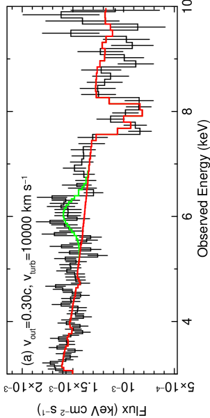
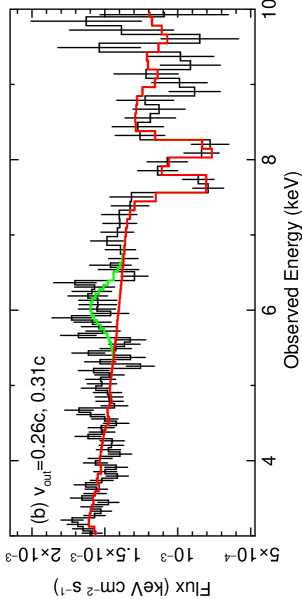
Figure 5: Comparison between outflowing Xstar models fitted to the Suzaku XIS–FI, showing the iron K band. Panel (a) shows a fit with one Xstar zone, outflowing with a single velocity of $v_{\rm out}=-0.30c$ and assuming a turbulence velocity of $v_{\rm turb}=10000$ km s^-1 (model A in Section 4.2). The absorption model is shown by the red line, the 8 keV absorption (observed frame) is modeled by a blend of Fe xxv and Fe xxv $1s-2p$ resonance lines, while iron K emission is shown in green. Panel (b) shows a similar model as per (a), but with two outflowing zones of $v_{\rm out}=-0.26c$ and $-0.31c$ (model B). Panel (c) shows a similar model as per panel (a), but with Gaussian velocity broadening included self-consistently for the iron K and L-shell emission and absorption (model C). The blue line shows the model without broadening. Further details are given in Section 4.2 and parameters for models A, B and C are listed in Table 3.

However one Xstar zone with a single outflow velocity does not quite accurately model the absorption profile shown in Figure 5a (plotted from 3–10 keV only for clarity), as the spacing between Fe xxv and Fe xxvi $1s-2p$ transitions (6.70 keV and 6.97 keV) is smaller than the observed separation of the absorption lines at 9.08 keV and 9.62 keV (rest-frame) respectively. Thus a better fit is subsequently obtained using two zones of absorbing matter, with different outflow velocities but assuming identical columns and ionizations. This model is referred to as model B, and is shown in Figure 5b. A column density of $N_{H}=(1.3\pm 0.5)\times 10^{24}$ cm^-2 is required, while a high ionization parameter of ${\rm log}\xi=4.9^{+0.9}_{-0.5}$ implies that iron is predominantly in a H-like state. The outflow velocities obtained are $v_{\rm out1}=-0.26\pm 0.02c$ and $v_{\rm out2}=-0.31\pm 0.02c$, while the fit statistic is good ($\chi^{2}/{\rm dof}=207.3/203$, null probability 0.4). Note that the presence of substantial columns of lower ionization gas (with $\log\xi<3$) fully covering the AGN are excluded, as this would produce considerable absorption from L-shell iron, as well as K-shell lines from Mg, Si and S below 3 keV, which are not observed in the Suzaku XIS spectrum. Low ionization gas, partially covering the emission below 10 keV during the Suzaku observation, can be excluded due to the lack of convex curvature in the XIS spectrum; however this is not the case for the 2001 XMM-Newton spectrum of PDS 456 discussed in Section 5.3.

We also allow both the iron emission and absorption to have the same self consistent velocity broadening, via convolution with a simple Gaussian broadening function, hereafter referred to as model C. This might be the case kinematically if the line emission is integrated over a smooth wide angle outflow or if the absorption is viewed over multiple lines of sight, e.g. if the absorber is extended with respect to the X-ray source, or if photons are scattered throughout the flow, as might be expected for the high columns observed here. This model can be expressed as:-

$$F(E)=[({\rm BPL}+{\rm GA}_{\rm em})\times{\rm XSTAR}(\xi,N_{\rm H},v_{\rm out})]\times{\rm GA}_{\rm conv}\times e^{-\sigma(E)N_{\rm H,Gal}}$$ (2)

where ${\rm GA}_{\rm conv}$ is the Gaussian broadening convolution. For simplicity a single bulk outflow velocity is assumed for the absorption, while the iron emission/absorption is assumed to be intrinsically narrow (prior to broadening), except for the turbulence velocity noted above. The resulting model is shown in Figure 5c, which has a velocity broadening of $26000\pm 7000$ km s^-1 (FWHM) and a net outflow velocity of $-0.29\pm 0.02c$. While this represents a statistically adequate fit ($\chi^{2}/{\rm dof}=227.9/205$, null probability 0.131), the model does not fit the profile of the absorption feature at 8 keV as well (c.f. model B), which appears narrower than the velocity broadening derived here. This might suggest that a homogeneous outflow is too simplistic and that significant clumping in the absorber may occur; this is discussed further in Section 6.

Alternatively we attempt to model the iron K absorption with no net outflow velocity, in the quasar rest frame at $z=0.184$. This is only plausible for very low values of the turbulence velocity (e.g. $\sigma_{\rm turb}\sim 100$ km s^-1 or less), so that the 9 keV rest-frame absorption is modeled by deep bound-free edges of Fe xxv and Fe xxvi, yet the equivalent widths of the corresponding $1s-2p$ absorption lines are small, as no absorption is observed in the spectrum at 6.70 or 6.97 keV (5.66, 5.89 keV observed frame). Indeed even the 99.7% confidence ($3\sigma$) upper-limits to any narrow absorption lines at these energies are -32 eV and -26 eV respectively (also including the broad iron K emission line as above).

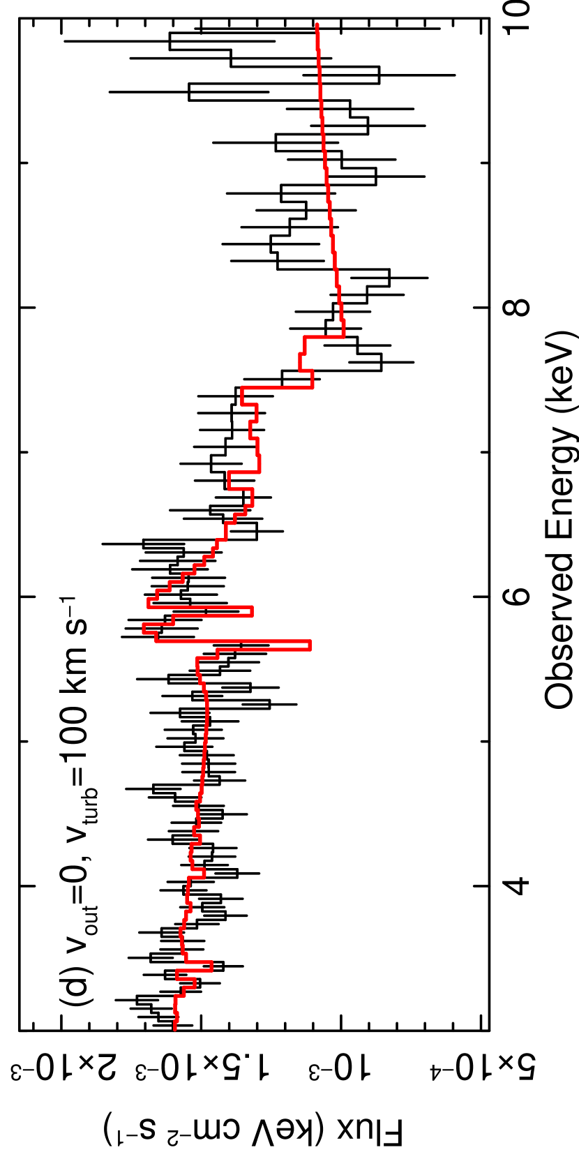
Figure 6: Xstar fit to the Suzaku XIS–FI data as per Figure 5, but with no net outflow velocity and assuming a very low turbulence velocity (100 km s^-1); e.g. model D in Section 4.2 and Table 3. A broad Fe K emission line is also included, as per models A-C in Figure 5. Here the absorption at 8 keV in the observed frame is modeled by bound-free edges from Fe xxv and Fe xxvi, from a high column density absorber (i.e. $\tau=1$), while narrow $1s-2p$ resonance lines from Fe xxv and Fe xxvi appear near 6 keV in the model (but not in the data). The fit is statistically worse than for the outflowing models shown in Figure 5 and such a small turbulence may be physically implausible.

Thus the high turbulence, high outflow velocity absorber from models A or B above is replaced by a low turbulence ($\sigma_{turb}=100$ km s^-1) absorber, with no net outflow velocity. The resulting model is listed as model D in Table 3. The broad iron K emission line is also included in model D as per models A–C. A high column density of $N_{\rm H}=1.2\pm 0.3\times 10^{24}$ cm^-2 and a high ionization of ${\rm log}\xi=4.0\pm 0.2$ is required in order to produce a deep absorption edge near 9 keV. Nonetheless the fit obtained with the low turbulence absorber is still worse than for the high velocity absorber in model B ($\chi^{2}/{\rm dof}=233.3.0/205$, vs $\chi^{2}/{\rm dof}=207.3.0/203$) and the model only crudely fits the profile of the absorption, as shown in Figure 6. If higher turbulences are assumed, e.g. 1000 km s^-1, the model predicts significant resonance $1s-2p$ absorption between 5.6-6.0 keV in the observed frame, which is not present in the data, resulting in a considerably worse fit of $\chi^{2}/{\rm dof}=267.5/205$.

One other possibility is that some narrow iron K emission just happens to cover up these $z=0.184$ rest frame absorption lines that are not seen in the spectrum. We denote this as model E in Table 3, which allows instead for two narrow (unresolved) emission lines at 6.70 keV and 6.97 keV rest frame in the spectrum; the fit statistic is slightly improved here ($\chi^{2}/{\rm dof}=228.4/204$), although this is still worse than model B ($\chi^{2}/{\rm dof}=207.3/203$). The fit with model E is worse still if a higher turbulence grid is used (e.g. $\sigma=1000$ km s^-1) as the predicted $1s-2p$ absorption lines are stronger, of EW 100 eV or more, while higher order (e.g. $1s-3p$) lines also become apparent and the fit statistic drastically worsens ($\chi^{2}/{\rm dof}=276.1/204$).

In conclusion we cannot completely rule out model D/E with zero outflow velocity, with these data, although this seems possible only for low turbulences (e.g. $100$ km s^-1, as per models D and E). It is also the case that such high column, high ionization gas would still be accelerated under the radiation pressure of the quasar, with an outward momentum rate of the order $L_{bol}/c$ (King & Pounds 2003), as such gas would have $\tau\sim 1$ to Thomson scattering and will likely not be static. We discuss this further in Section 6.4. Thus the most plausible origin of the absorption appears to be from highly blue-shifted iron K-shell lines of Fe xxvi or Fe xxv associated with a mildly relativistic outflow. Hereafter we adopt model B is the best parameterization of the iron K band absorption.

5 Modeling the Broad-Band Spectrum of PDS 456

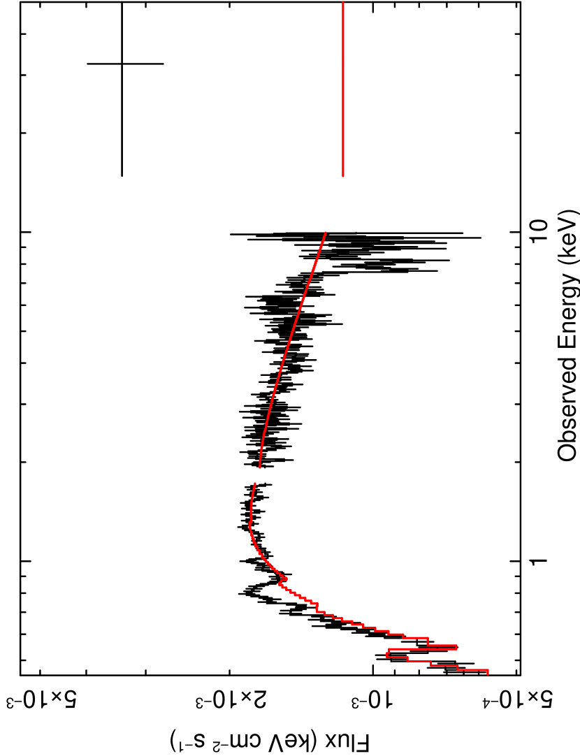
Figure 7: The Suzaku XIS and HXD spectra of PDS 456, plotted in $\nu F_{\nu}$ flux units. A factor of $\times 3$ excess is seen in the HXD, which may suggest that a Compton thick absorber, with $N_{\rm H}>10^{24}$ cm^-2 exists towards this optical type I quasar. The red line shows the extrapolation of the best-fit broken-powerlaw continuum extrapolated to higher energies.

PDS 456 appears to be weakly detected in the hard X-ray band, as described in Section 2, with an integrated 15–50 keV band flux of $7.3\pm 2.4\times 10^{-12}$ erg cm^-2 s^-1. This flux is somewhat higher than the flux measured by XIS ($3.8\pm 0.1\times 10^{-12}$ erg cm^-2 s^-1) in the 2–10 keV band. Indeed if we extrapolate the best fit XIS broken powerlaw continuum model in the previous section to higher energies, the predicted 15-50 keV flux is only $2.1\pm 0.2\times 10^{-12}$ erg cm^-2 s^-1. This possible factor of $\sim 3$ increase in flux above 10 keV is illustrated in Figure 7, which shows the extrapolation of the continuum fitted to XIS out to higher energies. The absolute level of the HXD flux is dependent on the background systematics of the detector, as discussed in Section 2, which we account for as an additional uncertainty on the HXD/PIN background level. After inclusion of this systematic error, the excess in HXD flux in Figure 7 appears significant at a moderate level of 99.8% confidence (corresponding to $\Delta\chi^{2}=13$), or about $3\sigma$. Further Suzaku HXD observations will hopefully confirm the validity of the hard X-ray detection of PDS 456.

5.1 Reflection Dominated Models

For now, we proceed by taking the HXD/PIN flux measurement at face value, noting that the fits below include the systematic error on the HXD/PIN background. Compton down-scattering or “reflection” off optically–thick matter (Lightman & White, 1988; George & Fabian, 1991), e.g. the disk or torus, could in principle account for the hard X-ray excess. We model this with Compton reflection off partially ionized material, using the reflion model (Ross et al., 1999; Ross & Fabian, 2005).

The emergent reflected spectrum is calculated for an optically-thick atmosphere (such as the surface of an accretion disk) of constant density illuminated by radiation with a power-law spectrum, with a high-energy exponential cutoff with an e-folding energy fixed at 300 keV, i.e. varying as $e^{-E/300{\rm keV}}$. The reflected spectrum is calculated over the range 1 eV to 1 MeV. Non-LTE calculations provide temperature and ionization structures for the gas that are consistent with the local radiation fields. In addition to fully-ionized species, the following ions are included in the calculations: C iii-vi, N iii-vii, O iii-viii, Ne iii-x, Mg iii-xii, Si iv-xiv, S iv-xvi, and Fe vi-xxvi. Thus the model self consistently computes the iron line (K or L-shell) emission, as well as from other elements.

The reflion model is also convolved with relativistic blurring from a disk around around a black hole (Fabian et al., 1989; Laor, 1991), to describe the reflected emission expected from the innermost accretion disk. A disk emissivity falling as $R^{-3}$ is assumed, along with an outer disk radius of $400R_{\rm g}$, where $R_{\rm g}$ is the gravitational radius. The model can be expressed as:-

$$F(E)=[{\rm CPL}+({\rm REF}\times\rm{KDBLUR})]\times\rm{XSTAR}(\xi,N_{\rm H},v_{\rm out})\times e^{-\sigma(E)N_{\rm H,Gal}}$$ (3)

where CPL is the illuminating cut-off powerlaw continuum, REF is the Compton reflected emission convolved with relativistic blurring (KDBLUR). Absorption from the putative high velocity outflow (denoted as XSTAR), is also included (modeled by an Xstar grid as per model B as described in Section 4.2) in order to account for the iron K-shell absorption at 9 keV.

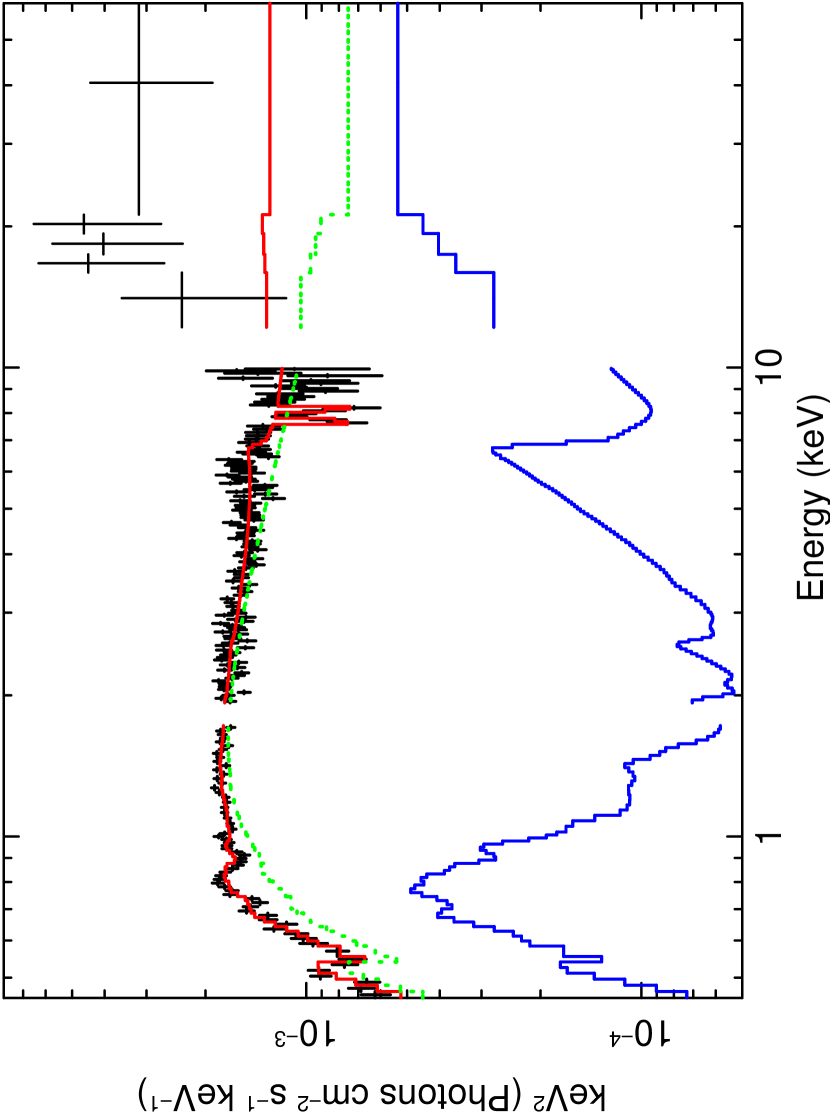
Figure 8: Suzaku XIS+HXD spectrum of PDS 456, fitted with an ionized disk reflection model, as described in Section 5.1. Data are shown in black, the blue line shows the blurred reflection component, green shows the intrinsic power-law continuum and red the total emission. Note the HXD/PIN spectrum is more finely binned than in Figure 7, at $\sim 2\sigma$ per bin above the background level.

An adequate fit ($\chi^{2}/{\rm dof}=248.5/212$, null probability $4.3\times 10^{-2}$) is obtained, with an inclination angle of $56\pm 8\hbox{${}^{\circ}$}$, an inner radius of $<20R_{\rm g}$, an ionization parameter of $\xi=190\pm 95$ and a power-law photon index of $\Gamma=2.32\pm 0.03$. The reflection fraction is then $R=\Omega/2\pi=1.3$, where $R=1$ corresponds to an infinite slab effectively subtending $2\pi$ steradian to the X-ray source. A high Fe abundance of $\times 4$ Solar is found, driven by the strong iron L-shell emission near 1 keV, although this value is not well constrained. Overall the fit is good below 10 keV, however the model fails to reproduce all of the excess in the HXD above 10 keV, see Figure 8, although the precise HXD/PIN flux is subject to systematic uncertainty as discussed above. Thus a contribution from a reflection component towards the X-ray emission from PDS 456 may be present, but does not appear to account for all of the hard X-ray emission observed in the HXD.

5.2 Absorption Models

An alternative scenario is that the majority of the intrinsic continuum flux from PDS 456 is in fact absorbed below 10 keV, therefore the heavily absorbed continuum only emerges above 10 keV and accounts for the observed hard X-ray excess. This is similar to the scenario in Seyfert 2s, where a heavily absorbed high energy continuum is often seen (Risaliti, 2002), except in PDS 456 the absorber must only partially cover the continuum X-ray emission in order for some direct flux below 10 keV to leak through, producing the observed continuum flux in the XIS. A similar, Compton-thick, but partially covering absorber has also recently been detected in the Suzaku HXD observation of the luminous AGN (at $z=0.104$), 1H 0419-577 (Turner et al., 2009). Any partial covering absorption must be located close to the central AGN, i.e. much closer than any pc scale absorber, in order to partially cover the compact X-ray emission.

In order to model this absorption we include a second layer of photoionized gas via the same Xstar grid as described in Section 4.2 (with solar abundances and $\sigma_{\rm turb}=10000$ km s^-1), in addition to the highly ionized absorption that is responsible for the iron K-shell lines at 9 keV. Thus this second layer of photoionized gas absorbs only a fraction $f$ of the intrinsic cut-off power-law continuum, while a fraction $1-f$ is not absorbed. Hence the model can be expressed as:-

$$F(E)=[({\rm CPL}\times f\times{\rm PC})+({\rm CPL}\times(1-f))+{\rm GA}_{\rm em}]\times{\rm XSTAR}(\xi,N_{\rm H},v_{\rm out})\times e^{-\sigma(E)N_{\rm H,Gal}}$$ (4)

where CPL is the cut-off powerlaw continuum with an e-folding energy of 300 keV, PC is the layer of absorbing gas that partially covers the X-ray source with a covering fraction $f$, while XSTAR represents the highly ionized outflowing gas that is responsible for the 9 keV iron K-shell absorption, which we assume to fully cover all of the X-ray emission. In this model the iron K and L-shell emission is included as Gaussian line components represented by ${\rm GA}_{\rm em}$. This model provides a statistically better fit ($\chi^{2}/{\rm dof}=217.9/209$, null probability 0.32), with a photon index of $\Gamma=2.27\pm 0.03$. A large column density is required to model the heavily absorbed component above 10 keV, with $N_{\rm H}=(3.5\pm 1.5)\times 10^{24}$ cm^-2 and an ionization parameter of log $\xi=2.5\pm 0.4$ erg cm s^-1; this lower ionization parameter value (log $\xi<3.0$) is required for the resulting continuum to be largely opaque below 10 keV, with most of the opacity arising from partially ionized iron (i.e. Fe xxiv and below). Likewise this sets the lower limit on the column density ($N_{\rm H}>2\times 10^{24}$ cm^-2). An outflow velocity for the partial covering absorption zone is not formally required, however it is not well constrained with a lower limit of $<0.2c$, less than for the highly ionized zone. The (line-of-sight) covering fraction of the absorber is $f_{cov}=0.72\pm 0.12$, i.e. $\sim 30$% is unabsorbed and this is the emission viewed below 10 keV.

Note that one drawback of the partially covering model discussed above, compared to the reflection model, is that the iron K and L-shell emission is not computed, instead we have simply parameterized the emission by Gaussians as discussed in Sections 3 and 4. However in the case of a Compton thick wind (i.e. with $N_{\rm H}>10^{24}$ cm^-2), significant emission via Compton reflection off the wind would be expected and could account for observed emission lines as well as the iron K band absorption. We discuss such a model further in Section 6.3.

5.3 Comparison with Previous Observations

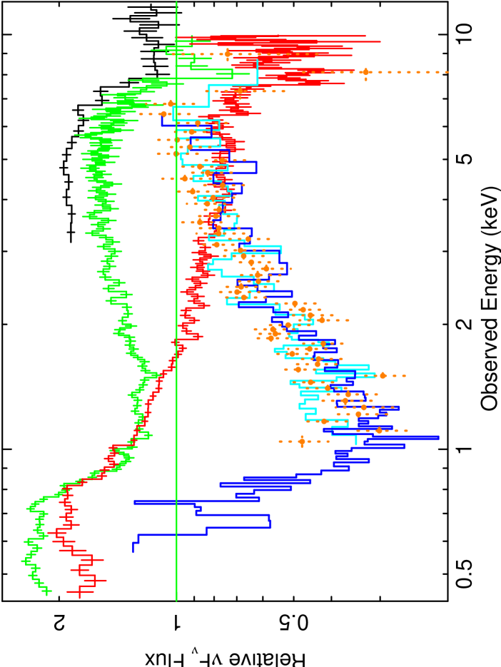
Figure 9: The current observations of PDS 456, shown as $\nu F_{\nu}$ spectra, where we have plotted the data compared to a ratio with an absorbed ($N_{\rm Gal}=2\times 10^{21}$ cm^-2) power-law of $\Gamma=2$ at a mean 2–10 keV flux level of $5\times 10^{-12}$ erg cm^-2 s^-1. Shown are RXTE PCA (black, 1998), XMM-Newton (2001, green), Suzaku XIS (2007, red), Chandra/HETG (2003, blue) and ASCA (1998, orange dotted). Strong variability is seen below 10 keV, from RXTE and XMM at high fluxes, down to Chandra and ASCA as the lowest/hardest observations. Note the 8 keV (observed) Fe K-shell absorption in the XMM–2001, Suzaku–2007 and RXTE–1998 observations. A summary of all these observations is shown in Table 1.

Variations in the absorption towards PDS 456 may also explain the drastic long term spectral variability of the AGN. Figure 9 shows the $\nu F_{\nu}$ spectral comparison between the Feb 2007 Suzaku observation with those by RXTE (1998/2001), ASCA (1998), XMM-Newton (2001) and Chandra (2003); see Table 1 for a list of observations. Below 10 keV, PDS 456 shows remarkable spectral variability. RXTE–1998 and XMM–2001 caught the AGN at a relatively high flux, as previously discussed. Reeves et al. (2003) derived a covering fraction of 60% for the absorber in the 2001 XMM-Newton observation, with a column density of $5.7^{+2.0}_{-2.5}\times 10^{23}$ cm^-2, an ionization parameter of log $\xi=2.5\pm 0.3$ and an outflow velocity of $\sim 50000$ km s^-1, although the latter value was not well constrained in the shorter 40ks observation. The low resolution RXTE/PCA spectra, from both 1998 and 2001, also show a deep absorption trough at 8 keV in the observed frame, with $\tau\sim 1$ implying a column density for the absorber of $\sim 10^{24}$ cm^-2 (Reeves et al., 2000). Interestingly the Beppo-SAX spectra of PDS 456 also show evidence for the highly ionized absorption between 8-9 keV (Vignali et al., 2000). We do not include the Beppo-SAX data in Figure 9, as the data are fairly noisy, but note that the spectra appear similar to those from XMM-Newton in 2001.

We re-analysed the XMM-Newton EPIC-pn spectrum from 2001, using the same Xstar grids as used in this current paper (with 10000 km s^-1 turbulence). The current grids have the advantage in that they include up to date opacities from partially ionized iron (Kallman et al., 2004); e.g. $1s-2p$ transitions from Fe xviii-xxiv and high order transitions from Fe xvii and lower. A model of the same form as the partial coverer in Section 5.2 was adopted. As per Suzaku XIS, a high ionization outflowing zone can fit the observed dip at 8 keV; with log $\xi=4.5\pm 0.5$, $N_{\rm H}=5\pm 2\times 10^{23}$ cm^-2 and $v_{\rm out}\sim-0.25c$. Interestingly partially covering absorption is also required in the XMM-Newton data to model the substantial continuum curvature present in the data from 1-10 keV (see Figure 9, green points), however the column density is lower ($N_{\rm H}\sim 1\times 10^{23}$ cm^-2) compared to the partial coverer in the Suzaku observation ($N_{\rm H}>10^{24}$ cm^-2). The partially covering gas is low ionization (log $\xi<2.1$) and does not produce strong $1s-2p$ lines from Fe xviii-xxiv, as the L-shell is filled, while its outflow velocity is not constrained by the pn data. The covering fraction of this absorber is measured to be 80%, very similar to the Suzaku value.

In contrast to this, the Chandra/HETG observation of PDS 456 in 2003 (and also ASCA in 1998) showed a very hard ($\Gamma=1.3$) low flux spectrum (i.e. XMM–2001, $F_{0.5-10}=1.1\times 10^{-11}$ erg cm^-2 s^-1; Chandra–2003, $F_{0.5-10}=4.0\times 10^{-12}$ erg cm^-2 s^-1). Changes in the covering and/or column of the (lower ionization) absorbing matter could possibly reproduce this spectral variability. For instance if the column density of the partial covering absorber was lower during the 2001 XMM-Newton observation, compared to the Suzaku observation (e.g. $N_{\rm H}\sim 10^{23}$ cm^-2 vs $>10^{24}$ cm^-2), this would allow more of the direct continuum to be observed below 10 keV, resulting in a higher flux during the XMM-Newton observation and accounting for the convex spectral shape below 10 keV. The lowest flux Chandra observation could also contain a greater contribution from the reflected emission, however any such component would have to be broadened as no narrow iron K-emission is observed. The long-term spectral variability of PDS 456, e.g. in the context of a variable partial covering absorber, will be investigated in more detail in a subsequent paper (Behar et al., 2009).

6 Discussion

6.1 The Intrinsic Luminosity of PDS 456

One possible consequence of the high column density absorption towards PDS 456 is that the intrinsic X-ray luminosity may be higher than inferred below 10 keV; the observed luminosity from 2–10 keV is only $4\times 10^{44}$ erg s^-1. In contrast the bolometric luminosity is substantially higher. From the optical spectrum of PDS 456 (Simpson et al., 1999) and correcting for the cosmology used in this paper, $\nu L_{\nu}(5100\AA)=2\times 10^{46}$ erg s^-1; thereby assuming a typical relation between the $5100\AA$ luminosity and the bolometric luminosity ($L_{\rm bol}$) of $L_{\rm bol}\sim 9\times\nu L_{\nu}(5100\AA)$ (Kaspi et al., 2000), an estimate of $L_{\rm bol}=1.8\times 10^{47}$ erg s^-1 for PDS 456 is derived. As a consistency check, we calculated the integrated infra-red to UV luminosity ($L_{\rm IR-UV}$) based on our previous spectra in the IR ($1-10\micron$), optical ($3000-8000\AA$) and UV ($1200-3000\AA$) bands (Simpson et al., 1999; O’Brien et al., 2005). The de-reddened $L_{\rm IR-UV}$ is $1.0\times 10^{47}$ erg s^-1, which defines a lower-limit on $L_{\rm bol}$, as the EUV band emission is not included. Thus hereafter we adopt $L_{\rm bol}=2\times 10^{47}$ erg s^-1 as the bolometric luminosity of PDS 456.

Hence the observed 2-10 keV luminosity measured by the XIS is only 0.2% of bolometric, meaning PDS 456 is X-ray faint compared to most quasars, where 3–5% of bolometric may be expected for a typical AGN SED (Elvis et al., 1994). This then suggests that part of the intrinsic X-ray emission may be hidden or absorbed, as discussed in the partial covering model, where 70% of the emission may be absorbed below 10 keV by a near Compton-thick layer of gas. Correcting for this putative absorption below 10 keV, the 2-10 keV luminosity is then $1.2\pm 0.3\times 10^{45}$ erg s^-1. Furthermore at the high column densities observed in PDS 456, the observed continuum X-ray flux may also be suppressed via by a factor $e^{-\tau}$, where $\tau=N_{\rm H}\sigma_{T}$ and $\sigma_{T}=6.65\times 10^{-25}$ cm² is the Thomson cross-section. Thus for a column of $N_{\rm H}=2\times 10^{24}$ cm^-2, derived from the Xstar fit to the absorber, then $\tau=1.3$ and thus the X-ray luminosity corrected for scattering and absorption is $L_{2-10}=4\times 10^{45}$ erg s^-1, about 2% of the bolometric luminosity of PDS 456. This value is consistent with the typical $\sim 3$% ratio between $L_{2-10}$ and $L_{\rm bol}$ measured for typical quasars (Elvis et al., 1994). This makes PDS 456 one of the most luminous known nearby quasars in the X-ray band similar to 3C 273, which is also consistent with its large bolometric luminosity, a factor of $\times 1.7$ higher than in 3C 273 in the optical band (Simpson et al., 1999).

6.2 An Outflow Model for PDS 456

Given the high ionization state (and possible partial covering) of the absorber in PDS 456, it is more likely to reside close to the X-ray emission region and not at parsec scales commensurate with the molecular torus, as predicted by AGN Unified schemes (Antonucci, 1993) and as suggested for some Seyfert outflows (Behar et al., 2003; Blustin et al., 2005).

Thus it is not likely to be the same matter responsible for the X-ray absorption towards Seyfert 2 galaxies, as PDS 456 is a classic luminous type I quasar with an unobscured view of the optical/UV BLR (Simpson et al., 1999; O’Brien et al., 2005). The X-ray absorber in PDS 456 is probably too highly ionized to cause significant absorption of the UV emission, although an outflowing absorption component to the Ly $\alpha$ line profile appears in the HST-STIS spectrum ($v=14000-24000$ km s^-1), as well as highly blue-shifted ($v=5000$ km s^-1) C iv emission (O’Brien et al., 2005). Thus one possibility is that the X-ray absorber is both part of a massive outflow, with density variations responsible for different gas layers. Dense ($n\sim 10^{10}$ cm^-3) clumps within the outflow can account for the possible Compton-thick absorption above 15 keV, which partially covers the X-ray emission, while the less dense (and highly ionized) fully covering gas is responsible for the strongly blue-shifted Fe K absorption lines. Indeed the high ionization gas may well shield the lower ionization matter.

We consider the case of a homogeneous radial outflow from PDS 456, in the form of a spherical flow (or some fraction $b$ there of). For simplicity, we assume that the outflow velocity is approximately constant on the compact scales observed here, although initial acceleration must occur close to the launch radius, with deceleration occurring at larger radii. From simple conservation of mass, the outflow rate is:-

$$\dot{M}_{\rm out}=4\pi bnR^{2}m_{p}v_{\rm out}$$ (5)

(where $nR^{2}=L_{\rm ion}/\xi$). Here $b=1$ for a full covering, homogeneous spherical outflow.

In PDS 456 the ionizing luminosity, defined by Xstar from $1-1000$ Rydberg with an input continuum of $\Gamma=2.2$ is $L_{\rm ion}=3\times 10^{45}$ erg s^-1, correcting for Galactic absorption. This luminosity may indeed by higher by a factor of 3, e.g. if 70% of the emission below 10 keV is absorbed or scattered. However in the calculations below we adopt $L_{\rm ion}=3\times 10^{45}$ erg s^-1 as a robust lower limit to this luminosity.

As discussed in Section 4.2, the high ionization matter appears to be outflowing with $v_{\rm out}=-0.26c$, with an ionization parameter of log $\xi=4.9$; e.g. see model B, Table 3. Thus the outflow rate in PDS 456 is of the order $\dot{M}_{\rm out}=6\times 10^{27}b$ g s^-1 or $100b\hbox{$\rm~{}M_{\odot}$}$ yr^-1. Even for a rather conservative value of $b\sim 0.1$, then $\dot{M}_{\rm out}\sim 10\hbox{$\rm~{}M_{\odot}$}$ yr^-1. The outflow kinetic power is then simply $\dot{E}_{\rm out}\sim\dot{M}_{\rm out}v_{\rm out}^{2}/2$, which is then $2\times 10^{47}b$ erg s^-1. Thus the kinetic output of the wind may be an appreciable fraction of the bolometric luminosity for PDS 456 for a reasonable value of $b$. Note that the kinetic power is very sensitive to $v_{\rm out}$, effectively varying as $v_{\rm out}^{3}$, but note that we adopt the lowest value of the likely velocity range $v_{\rm out}=0.26-0.31c$ derived in Table 3.

There is no direct (e.g. reverberation) mass estimate for the black hole in PDS  456, however we can estimate its likely value from known scaling relations, derived from reverberation methods, between the AGN BLR virial radius and black hole mass (Kaspi et al., 2000; McLure & Jarvis, 2002). If we adopt the relation derived in McLure & Jarvis (2002):-

$$M_{\rm BH}=4.74(\lambda L_{5100\AA}/10^{44}{\rm erg\,s}^{-1})^{0.61\pm 0.10}[{\rm FWHM}(H\beta)]^{2}\hbox{$\rm~{}M_{\odot}$}$$ (6)

where $\lambda L_{5100\AA}=2\times 10^{46}$ erg s^-1 and ${\rm FWHM}(H\beta)=3974\pm 764$ km s^-1 (Torres et al., 1997; Simpson et al., 1999), then the black mass is ${\rm log}M_{\rm BH}=9.3\pm 0.4\hbox{$\rm~{}M_{\odot}$}$ for PDS 456. Alternatively, using the equivalent relation in Kaspi et al. (2000) gives ${\rm log}M_{\rm BH}=9.5\pm 0.3\hbox{$\rm~{}M_{\odot}$}$. The Eddington-limited luminosity for an accreting black hole of mass $M_{\rm BH}$ is $L_{\rm Edd}=4\pi GMm_{\rm p}c/\sigma_{T}$, while the Eddington accretion rate is simply $\dot{M}_{\rm Edd}=L_{\rm Edd}/(\eta c^{2})$, where $\eta$ is the efficiency of converting rest-mass into energy. For PDS 456 if $M_{\rm BH}=2\times 10^{9}\hbox{$\rm~{}M_{\odot}$}$, then $L_{\rm Edd}=2\times 10^{47}$ erg s^-1 and $\dot{M}_{\rm Edd}=50\hbox{$\rm~{}M_{\odot}$}$ yr^-1 for $\eta=0.06$ (the maximum efficiency for accretion onto a Schwarzschild black hole). Thus the mass outflow rate is likely to be a substantial fraction of the total accretion rate.

The escape radius of the outflow is simply $R_{\rm esc}\sim(2c^{2}/v^{2})R_{g}>30R_{\rm g}$ (where $R_{\rm g}=GM_{\rm BH}/c^{2}$ is the gravitational radius), equivalent to $R_{\rm esc}=10^{16}$ cm for $M_{\rm BH}=2\times 10^{9}\hbox{$\rm~{}M_{\odot}$}$. For the case of a homogeneous radial outflow, the density varies as $n\propto R^{-2}$ and thus the ionization parameter $\xi=L/nR^{2}$ is largely independent of the outflow radius. Hence the column density viewing through the line of sight down to a characteristic wind radius $R_{\rm wind}$, for the case of a spherical or bi-conical flow viewed radially, is:-

$$N_{\rm H}=\int_{\rm R_{wind}}^{\infty}n(R)dR=\int_{\rm R_{wind}}^{\infty}(L_{\rm ion}/\xi R^{2})dR=L_{\rm ion}/\xi R_{\rm wind}$$ (7)

Therefore for PDS 456, as $N_{\rm H}\sim 10^{24}$ cm^-2 and log $\xi=4.9$, then $R_{\rm wind}=3\times 10^{16}{\rm cm}\sim 100R_{\rm g}$. Note $R_{\rm wind}$ is within the expected UV/BLR emission radius for PDS 456; e.g. for ${\rm FWHM}({\rm Ly}_{\alpha})=12000$ km s^-1 (O’Brien et al., 2005), then $R_{\rm UV}\sim 1000R_{\rm g}$. Note that as the highly ionized matter is located close to the black hole in PDS 456, this likely excludes the possibility of low turbulence (and low outflow velocity) gas (model D, Section 4.2) contributing towards the iron K band absorption.

It is also possible that the wind is not homogeneous but is instead clumpy. Indeed X-ray variability is observed in PDS 456 on rapid ($20-30$ ks) timescales, e.g. as seen previously in the XMM-Newton, Beppo-SAX or RXTE observations (Reeves et al., 2000, 2002) and in the current Suzaku XIS observation, which implies a compactness on sizescales of several $R_{\rm g}$. Thus we consider the case where the absorption derives from clumps of matter of approximately constant density. In this scenario the maximum distance of the clumps ($R_{\rm max}$) is given by $\Delta R/R_{\rm max}<1$, where $\Delta R$ is the clump thickness. Now $N_{\rm H}=n\Delta R$ and $n=L_{\rm ion}/\xi R_{\rm max}^{2}$ as before; thus we derive the condition that $R_{\rm max}<L_{\rm ion}/N_{\rm H}\xi$ and so $R_{\rm max}<100R_{\rm g}$ for $\Delta R/R_{\rm max}<1$. Thus for $R=30R_{\rm g}$, $n=3\times 10^{8}$ cm^-3 and $\Delta R/R=0.3$. Indeed the fact that both high ionization ($\log\xi=4.9$) and lower ionization (partially covering) gas (with $\log\xi<3$) is observed in the Suzaku and 2001 XMM-Newton spectra does suggest that the absorbing matter is inhomogeneous. The gas may also become less ionized to larger radii, especially if the outer layers are shielded from the photoionizing X-ray source. Such matter could contribute towards the blue-shifted Lyman $\alpha$ absorption and C iv emission seen in the HST/STIS spectrum of PDS 456 (O’Brien et al., 2005), although with columns much smaller than those derived here.

6.3 Outflow Emission and Energetics

It may be plausible that the outflowing gas produces both the Fe L and K-shell emission. The emission could occur via transmission, but given the high column densities involved, more likely through reflection off the surface of the wind. To test this, we constructed a similar model to the Compton-thick absorber model in Section 5.2, with two absorbing layers; one representing a very high ionization outflowing zone and a lower ionization partial covering zone (e.g. representing denser clumps within the wind). However in addition to the absorption, the model also allows for some reflected emission (via the reflion model) from high ionization matter to represent possible scattering off the wind. The illuminating continuum is then just a single power-law of $\Gamma=2.25\pm 0.03$. The reflection component is also convolved through a simple Gaussian velocity-broadening function (with $\Delta E/E$ constant with energy). This accounts for the line broadening clearly visible in the 7 keV and 1 keV emission lines detected by XIS. The model can be expressed as:-

$$F(E)=[({\rm CPL}\times f\times{\rm PC})+({\rm CPL}\times(1-f))+({\rm REF}\times{\rm GA}_{\rm conv})]\times\rm{XSTAR}\times e^{-\sigma(E)N_{\rm H,GAL}}$$ (8)

where CPL is the cut-off powerlaw with $E_{\rm cut}=300$ keV, PC is the partially covering absorber with a covering fraction $f$, XSTAR is the highly ionized outflowing absorber, REF is the reflected emission off partially ionized matter and ${\rm GA}_{\rm conv}$ corresponds to the Gaussian velocity convolution for the reflected emission.

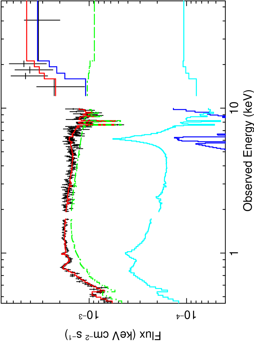
Figure 10: Model fitted to the Suzaku spectrum, representative of absorption and emission from a high column density disk wind, as described in Section 6.3, with model parameters listed in Table 4. Datapoints are shown in black, the dotted green line represents the power-law ($\Gamma=2.2)$ continuum that is absorbed only by the very high ionization fast outflowing zone, the dark blue line is the continuum obscured by the partial covering absorber which covers 80% of the X-ray source, the light-blue line is the reflected emission off the Compton-thick partially ionized wind and red is the total emission from all components.

This model is shown in Figure 10 and the fit parameters are summarised in Table 4 (the “outflowing wind” model). A good fit is obtained ($\chi^{2}/{\rm dof}=217.3/211$) and the model well reproduces both the absorption in the XIS and HXD spectra as well as the ionized iron L and K-shell emission and the general shape of the continuum. The ionization derived for the reflector is high, with log $\xi=3.0\pm 0.3$ erg cm s^-1, which is intermediate between the high ionization outflowing absorber and the partial coverer. The ionized reflector represents approximately 20% of the broad-band flux of the power-law continuum and hence has $R=0.2$, but contributes less at energies above 10 keV due to the high ionization of this component. Thus the scattered component may cover a solid angle corresponding to $b\sim 0.2$ for significant emission to be observed in the Suzaku spectrum. We note that a value of $b=0.3$ was recently derived for the outflow in PG 1211+143, via a P-Cygni like profile to the iron K absorption line, suggesting that the kinetic power of the outflow in that quasar is also likely to be similar to its total bolometric output (Pounds & Reeves, 2009).

Note that velocity broadening is required for the reflected emission, corresponding to 35000 km s^-1, driven by the widths of the emission lines in the spectrum, while some net outflow of the reflector is also preferred (see Table 4). The velocity broadening may arise from the integrated emission expected over a wind with appreciable solid angle. A future comparison with disk wind models being developed that fully incorporate self-consistent radiative transfer calculations for both the emission and the absorption (Sim et al., 2008; Schurch et al., 2009) may prove to be interesting.

As a consistency check we compare the mass outflow rate calculated in Section 6.2 with that predicted via transfer of momentum through radiation pressure, assuming that the wind is radiatively driven. For such a high ionization outflow, the predominant form of momentum transfer to the wind will be through scattering (King & Pounds, 2003), whereby:-

$$\dot{M}_{\rm out}v_{\rm out}=\frac{L_{\rm Edd}}{c}(1-e^{-\tau})$$ (9)

where $\tau\sim 1$ as measured in the Suzaku spectrum of PDS 456 and $L_{\rm Edd}=2\times 10^{47}$ erg s^-1 (see Section 6.1). Thus from the above $\dot{M}_{\rm out}v_{\rm out}=4.5\times 10^{36}$ g cm s^-2 and as $v_{\rm out}=0.26c$, then the mass outflow rate is $\dot{M}_{\rm out}=6\times 10^{26}$ g s^-1 or $\sim 10\hbox{$\rm~{}M_{\odot}$}$ yr^-1. In comparison the mass outflow rate calculated in Section 6.2 (equation 5) is $\dot{M}_{\rm out}=6b\times 10^{27}$ g s^-1 and thus $b\sim 0.1$ for PDS 456, consistent with the estimate from the above model. Behar et al. (2009) derive a global covering fraction of $b=0.2$ for the highly ionized absorber/reflector, by considering the reflected emission in all the observations of PDS 456 to date.

If $b\sim 0.2$, then the outflow is energetically significant, with a kinetic power of $\dot{E}=4\times 10^{46}$ erg s^-1. Integrated over a quasar lifetime of $10^{8}$ years and if we assume a conservative duty cycle of 10% for the outflow to be active, then the total amount of energy released by the wind will be $\sim 10^{61}$ erg, plausibly exceeding the binding energy of a galaxy bulge of mass $10^{11}\hbox{$\rm~{}M_{\odot}$}$ and velocity dispersion $\sigma=300$ km s^-1 of $5\times 10^{59}$ erg. Thus such powerful winds could potentially cause significant feedback between the galactic bulge and black hole during the quasar phase.

The duty cycle for the outflow is largely unknown, however we know that the iron K absorption was detected in most of the observations of PDS 456 to date (see Figure 7). There are also several reported cases of high velocity outflows that are emerging in the literature, e.g. Cappi (2006); Reeves et al. (2008) and references therein. The frequency of these winds and how the outflow depends on critical parameters (such as accretion rate) awaits a more systematic and statistically rigorous survey of such systems in the Suzaku and XMM-Newton archives. Future calorimeter based X-ray spectra with Astro-H and IXO, with resolution $E/\Delta E>1000$ at 6 keV, will hopefully reveal a wealth of information on these outflows in the iron K band.

6.4 Is a low velocity solution plausible for the Fe K absorption?

Finally we consider whether it is plausible for a low velocity, low turbulence absorber to cause the iron K-shell absorption in PDS 456 and not a high velocity wind. The first apparent problem is that the high column, high ionization gas will naturally be accelerated under the radiation pressure from the central quasar. For the column densities here, the gas has an optical depth of $\tau\sim 1$ to Thomson scattering. In this scenario the outward rate of momentum transferred to the gas will be equivalent to $\dot{M}_{\rm out}v_{\rm out}\sim L_{\rm Edd}/c$, e.g. see King & Pounds (2003), King (2003). For PDS 456, $L_{\rm Edd}\sim L_{\rm bol}=2\times 10^{47}$ erg s^-1 and hence the outward momentum rate for the wind is $\dot{M}_{\rm out}v_{\rm out}\sim 10^{37}$ g cm s^-2. For low velocity gas, e.g. $v_{\rm out}=-100$ km s^-1 as per model D or E, then the mass outflow rate will subsequently need to be huge for the above Thomson case, i.e. $\dot{M}_{\rm out}\sim 10^{30}$ g s^-1 (or $10^{4}M_{\odot}$ yr^-1) for the gas not to be outflowing with greater velocities. This value is then inconsistent with the mass outflow rate of $\sim 10^{25}$ g s^-1 calculated from equation (5), for $v_{\rm out}=-100$ km s^-1 and log $\xi=4$. In comparison for an outflow velocity of $v_{\rm out}=-0.25c$ as per models A–C, the mass outflow rate derived from the Thomson case above is consistent with the value derived from equation (5), i.e. $\dot{M}_{\rm out}\sim 10^{27}$ g s^-1. It may be possible for the gas to be shielded from the central source, so as not to be accelerated by the radiation pressure, however given the high degree of ionization of the X-ray absorber this appears unlikely.

Secondly, the radial distance from the black hole to the wind is unlikely to be substantially greater than $100R_{\rm g}$, as discussed in Section 6.2. At this distance, it seems somewhat implausible that the highly ionized gas will have velocities as low as 100 km s^-1, as is required for models D and E.

Finally no narrow absorption has been observed in any of the X-ray or UV observations of PDS 456 to date (e.g. Reeves et al. 2003; O’Brien et al. 2005; Behar et al. 2009). In the HST-STIS observation of PDS 456 (O’Brien et al. 2005), the broadened Lyman$-\alpha$ absorption line has an outflow velocity of $-(14000-24000)$ km s^-1 and a simple Gaussian fit to the absorption line profile reveals a width of $8000\pm 1400$ km s^-1 (FWHM) corresponding to $\sigma=3400\pm 600$ km s^-1. The XMM-Newton RGS spectrum from a 2001 observation has been re-analysed by Behar et al. (2009), who report evidence for absorption from Ne ix and Fe xx, with a corresponding outflow velocity of $-16000\pm 1500$ km s^-1 and a width of $\sigma=2500$ km s^-1. These values are consistent with the HST-STIS UV spectrum, but while the gas is lower ionization and not likely to be responsible for the Fe xxv-xxvi K-shell absorption observed in Suzaku, it does suggest the absorption seen towards PDS 456 is likely high velocity and highly turbulent. Finally the 9 keV rest frame iron K-shell absorption in this Suzaku observation, as reported in Sections 3 and 4, also appears to be broadened. Thus it appears unlikely that narrow, low velocity gas contributes significantly to the X-ray absorption observed towards PDS  456.

7 Conclusions

We have detected the signature of a possible Compton thick wind from PDS 456, a high luminosity nearby quasar ($z=0.184$) which accretes near to the Eddington limit. The Suzaku XIS spectrum shows evidence for statistically significant (at $>99.9$% confidence) absorption in the Fe K band, which can be modeled by a pair of absorption lines (or one broad line) near 9 keV in the quasar rest frame. The large velocity shift, compared to the most likely identification of the absorption with Fe xxvi ($1s-2p$) at 6.97 keV, implies an outflow velocity of $0.26-0.31c$. As has been discussed in detail, an identification with other atomic transitions is less likely and the large outflow velocity appears to be required. The large velocity implies that the mass outflow rate is high, of the order of several tens of Solar masses per year, with a corresponding kinetic power of up to $\sim 10^{47}$ erg s^-1, close to the Eddington-limited luminosity of PDS 456. Such winds could be an important source of feedback regulating black hole and bulge growth (King, 2003; Di Matteo et al., 2005) during the quasar growth phase in the early Universe.

A tentative hard X-ray detection of PDS 456 above 15 keV has also been made (at the $\sim 3\sigma$ level) in the HXD/PIN, at a low flux level of $7\times 10^{-12}$ erg cm^-2 s^-1. The hard X-ray emission requires either a Compton-thick ($N_{\rm H}>10^{24}$ cm^-2) partial covering absorber or strong reflection, or a combination of both, to account for the apparent hard X-ray excess. However at the current low significance level of the detection, a further deep observation of PDS 456 with Suzaku is needed to confirm the nature of the hard X-ray excess.

8 Acknowledgements

We would like to dedicate this paper to the memory of Professor Martin Turner CBE. This research has made use of data obtained from the Suzaku satellite, a collaborative mission between the space agencies of Japan (JAXA) and the USA (NASA). We would also like to thank Alex Markowitz for kindly reprocessing the archived RXTE spectra of PDS 456. E.B. was partially supported by NASA grant No. 08-ADP08-0076 issued through the Astrophysics Data Analysis Program (ADP), while T.J.T was partially supported by NASA grant NNX08AJ41G. SK is supported at the Technion by the Kitzman Fellowship and by a grant from the Israel-Niedersachsen collaboration program.

Appendix A - Possibility of HXD Contamination

It is important to discuss the possibility of contaminating X-ray emission from other sources within the HXD field of view. Nonetheless there are no known bright ($F_{2-10}>10^{-13}$ erg cm^-2 s^-1) contaminating point sources from previous imaging observations of PDS 456 below 10 keV, e.g. with ASCA GIS, SAX/MECS, XMM-Newton EPIC which have similar fields of view to Suzaku/HXD. Above 10 keV, no known hard X-ray sources (other than the expected detection of PDS 456 itself) are present within $2\hbox{${}^{\circ}$}$ of PDS 456 in the RXTE slew survey (Revnivtsev et al., 2004) nor from the Integral/IBIS all sky survey (Krivonos et al., 2007a). The nearest known source detected in the Integral all sky survey is the LMXB, GX 9+9, approximately $3\hbox{${}^{\circ}$}$ from PDS 456. There is a possibility of some weak Galactic diffuse contamination due to the position of PDS 456, at the very edge of the Galactic bulge, $l=10.4\hbox{${}^{\circ}$}$, $b=+11.2\hbox{${}^{\circ}$}$), due to a population of accreting magnetic CVs. Results from the Integral (Krivonos et al., 2007b) or RXTE/PCA (Revnivtsev et al., 2006) Galactic ridge surveys show that this contributes $<1\times 10^{-12}$ erg cm^-2 s^-1 from 15-50 keV, integrated over the much smaller HXD/PIN field of view and thus is negligible.

There is also the contribution of Extragalactic diffuse (AGN) emission from the Cosmic hard X-ray Background (CXB), an estimate of which has already been included in the background spectrum for the HXD/PIN. The HXD detection of PDS 456 lies above the level expected from the CXB. The flux measured by the HXD, minus the non X-ray background (NXB) component (but not the CXB) is $1.52\pm 0.20\times 10^{-11}$ erg cm^-2 s^-1 (15-50 keV band). In this paper we have adopted the expected CXB flux from the HEAO-1 measurement of Gruber et al. (1999), which is $7.9\times 10^{-12}$ erg cm^-2 s^-1 from 15-50 keV, thus the net intrinsic flux from PDS 456 is $7.3\pm 2.4\times 10^{-11}$ erg cm^-2 s^-1. The error includes the 1.3% absolute uncertainty in the HXD/PIN background, and allows for 10% uncertainty in the CXB determination. Note that the CXB flux measured by Gruber et al. (1999) is also consistent with that obtained by Beppo-SAX PDS by Frontera et al. (2007), who obtain a 90% upper bound on the CXB level of $6.5\pm 0.2\times 10^{-8}$ erg cm^-2 s^-1 sr^-1 (20-50 keV) equivalent to $8.3\pm 0.2\times 10^{-12}$ erg cm^-2 s^-1, when normalized to the Suzaku HXD field of view and converted to the 15-50 keV band. We note that the Integral IBIS measurement of the CXB, by Churazov et al. (2007) via Earth occultation, is also within 10% of the HEAO-1 measurement. The effect of any anisotropy of the CXB should be negligible, fluctuations are thought to be at the level of 5–10% on scales of a square degree. As a final check of the CXB level, we also computed the HXD flux from the Suzaku observation of the Lockman Hole (LH), performed on 3–6 May 2007. The data were reduced as described in Section 2, resulting in 84.3 ks of net HXD exposure. The HXD/PIN spectrum of PDS 456 lies significantly above that of the LH emission, while the LH flux is consistent with the expected CXB level ($0.9\pm 0.2\times 10^{-11}$ erg cm^-2 s^-1). Thus uncertainty in the CXB subtraction does not significantly effect the detection of PDS 456.

One final possibility is that a bright, serendipitous AGN is located within the HXD field of view. From the the Swift–BAT hard X-ray selected AGN $logN-logS$ (Tueller et al., 2008), we would randomly expect $<5\times 10^{-3}$ AGN of flux $\sim 1\times 10^{-11}$ erg cm^-2 s^-1 per HXD field. The actual probability is likely much lower, as there are no other bright AGN candidates in the soft X-ray ($<10$ keV) or optical fields of view. Thus in order to contaminate the HXD/PIN field of view, a background AGN would itself have to be heavily absorbed ($N_{\rm H}>10^{24}$ cm^-2) below 10 keV (so that $F_{2-10}\mathrel{\hbox{\hbox to0.0pt{\hbox{\lower 4.0pt\hbox{$\sim$}}\hss}\hbox{$<$}}}10^{-13}$ erg cm^-2 s^-1, as there are no known bright source in the PDS 456 field below 10 keV) and yet its spectrum must rise by a factor of $\times 100$ above 10 keV. Statistically speaking, $<5$% of the BAT selected AGN have $N_{\rm H}>10^{24}$ cm^-2, meaning that the coincidence probability is $\sim 10^{-4}$. The only other possibility is of a flaring object, such as a blazar, brightening during the observation, although the HXD lightcurve is flat (Figure 1), which appears to exclude this and also the object would have to be located outside the imaging field of view of the XIS.

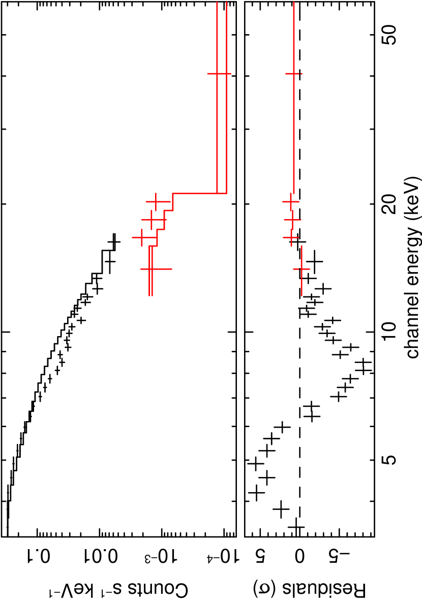
Figure 11: A comparison between the time–averaged RXTE/PCA spectrum between 3–18 keV and the HXD/PIN Suzaku spectrum from 15–50 keV. The plot shows the comparison of the data to a $\Gamma=2.2$ continuum with Galactic absorption, with no re-normalization of either spectrum, while the lower panel shows the residuals between the data and the model. Although the RXTE/PCA data is non simultaneous with the HXD (see Table 1 for a list of observations), the PCA spectrum below 18 keV extrapolates well to the HXD/PIN data above 15 keV. Also notice the deep absorption trough centered at 8 keV in the RXTE/PCA spectrum, consistent with the absorption in the 2007 Suzaku XIS and 2001 XMM-Newton data.

Furthermore, PDS 456 was also detected previously in both 1998 (Reeves et al., 2000) and 2001 with RXTE, with a hard X-ray flux of $F_{3-15}=0.7-0.9\times 10^{-11}$ erg cm^-2 s^-1. PDS 456 was also more recently detected in a 35 ks worth of RXTE pointings in 2008 (see Table 1 for a list of observations). PDS 456 was not detected in a previous observation with Beppo-SAX PDS (Feb 2001, 71 ks PDS exposure), however the upper limit obtained is consistent with the above HXD analysis ($F_{20-100}<1.5\times 10^{-11}$ erg cm^-2 s^-1). Indeed although the RXTE observations and the Suzaku HXD observation are not simultaneous (see Table 1), the time-averaged RXTE/PCA spectrum extrapolates very well to the HXD/PIN measurement (see Figure 11). Therefore it appears likely that the detected hard X-ray emission is due to the quasar and not due to any contaminating sources in the field of view.

Figure 1: (a) Comparison between the background A model and the Earth occultation data for HXD/PIN (from $15-50$ keV, where the light curve represents the ratio between the (Earth - Bgd A) / Bgd A rate. The background A model underpredicts the Earth background by $8.8\pm 1.0$%. (b) Comparison between the background D model and the Earth occultation data, where the light curve represents the ratio between the (Earth $-$ Bgd D) / Bgd D rate. The background D model slightly underpredicts the Earth background by $2.4\pm 1.0$%. (c) The net 15-50 keV HXD/PIN lightcurve using the background D model, the CXB background level (0.17 cts s^-1) is marked by a horizontal line.

Table 1: Summary of PDS 456 Observations

Telescope	Modea	Start Date/Timeb	End Date/Timeb	Exposurec	$F_{2-10}$d
Suzaku XIS	XIS nom	2007/02/24 17:58:04	2007/03/01 00:51:14	179.6	3.7
Suzaku HXD/PIN	–	–	–	164.8	–
XMM-Newton pn	FW/med	2001/02/26 10:46:57	2001/02/26 22:00:41	36.4	6.9
Chandra/HETG		2003/05/07 03:29:56	2003/05/08 20:08:33	142.8	3.8
ASCA/SIS		1998/03/07 09:06:36	1998/03/08 14:58:42	42.8	4.0
RXTE/PCA		1998/03/07 17:07:44	1998/03/10 07:50:56	92.1	8.1
		2001/02/23 04:20:32	2001/03/11 05:59:44	168.3	10.4
		2008/02/22 21:00:32	2008/11/14 08:17:36	34.7	6.9
Beppo-SAX/PDS		2001/02/26 09:50:03	2001/03/03 08:57:30	71.0	–

Table 2: Spectral Parameters to Suzaku XIS

Model Component	Fit Parameter	Value	$\Delta\chi^{2}$a
1. Broken Power-law Continuumb	$\Gamma_{\rm soft}$	$2.44\pm 0.04$
	$E_{\rm break}$	$2.0\pm 0.2$
	$\Gamma_{\rm hard}$	$2.24\pm 0.02$
	$N_{\rm BPL}$	$(2.4\pm 0.1)\times 10^{-3}$
	$F_{0.5-10keV}$	$7.2\times 10^{-12}$
2. Galactic Absorptionc	$N_{\rm H}$	$(2.2\pm 0.2)\times 10^{21}$
3. Soft X-ray Emission Linesd	$E_{\rm line}$	$0.91\pm 0.01$	174.4
	Line Flux	$(2.0\pm 0.4)\times 10^{-4}$
	EW	$42\pm 10$
	$\sigma$	$0.075\pm 0.015$
Second line	$E_{\rm line}$	$1.16\pm 0.02$	17.7
	Line Flux	$(1.4\pm 0.6)\times 10^{-5}$
	EW	$6\pm 3$
	$\sigma$	$0.01^{f}$
4. Iron K Absorption Linesd	$E_{\rm line}$	$9.09\pm 0.05$	41.1
	Line Flux	$-3.0^{+1.5}_{-1.1}\times 10^{-6}$
	EW	$133\pm 39$
Second line	$E_{\rm line}$	$9.64\pm 0.08$	29.0
	Line Flux	$-(2.5\pm 1.0)\times 10^{-6}$
	EW	$129\pm 48$
	$\sigma$	$0.105^{+0.055}_{-0.065}$ (tied to first line)
5. Iron K Emission Lined	$E_{\rm line}$	$7.1\pm 0.2$	27.7
	Line Flux	$(5.1\pm 2.0)\times 10^{-6}$
	EW	$133\pm 52$ eV
	$\sigma$	$0.35^{+0.65}_{-0.14}$
Fit statisticse	$\chi^{2}/{\rm dof}$	$431.5/374$
	Null probability	$2.1\times 10^{-2}$

Table 3: Xstar Photoionization Model Fits to Suzaku XIS

Modela	$N_{H}$b	log $\xi$c	$\sigma_{\rm turb}$d	$v_{\rm out}$e	$v_{\rm broad}$f	$\chi^{2}/{\rm dof}$g	Null Probg
A	$0.22^{+0.11}_{-0.10}$	$4.1\pm 0.2$	10000	$-0.30\pm 0.02c$	–	224.9/204	0.151
B	$1.3\pm 0.6$	$4.9^{+0.9}_{-0.5}$	10000	$-0.26\pm 0.02c$	–	207.3/203	0.394
	tied	tied	tied	$-0.31\pm 0.02c$
C	$1.5\pm 0.6$	$4.4\pm 0.4$	10000	$-0.29\pm 0.02c$	$26000\pm 7000$	227.9/205	0.131
D	$1.2\pm 0.3$	$4.0\pm 0.2$	100	0	–	233.3/205	$8.5\times 10^{-2}$
E	$1.3\pm 0.5$	$4.0\pm 0.2$	100	0	–	228.3/204	0.118

Table 4: Outflowing Wind Model Parameters

Model Component	Fit Parameter	Value
1. Power-law Continuum	$\Gamma$	$2.25\pm 0.05$
	$N_{\rm abs}$a	$(8.1\pm 2.3)\times 10^{-3}$
	$N_{\rm unabs}$a	$(2.0\pm 0.1)\times 10^{-3}$
	$F_{0.5-10keV}$b	$7.2\times 10^{-12}$
	$F_{15-50keV}$b	$7.8\times 10^{-12}$
2. Outflowing Fe K-shell Absorber	$N_{\rm H}$c	$(1.3\pm 0.5)\times 10^{24}$
	log $\xi$d	$4.9^{+0.9}_{-0.5}$
	$v_{\rm out1}$e	$-0.26\pm 0.02c$
	$v_{\rm out2}$e	$-0.31\pm 0.02c$
3. Compton-thick Hard X-ray Absorber	$N_{\rm H}$c	$>2.5\times 10^{24}$
	log $\xi$d	$2.5\pm 0.4$
	$f_{\rm cov}$f	$0.80^{+0.04}_{-0.07}$
4. Ionized Reflection	log $\xi$d	$3.0\pm 0.3$
	$v_{\rm broad}$g	$35000\pm 17000$
	$v_{\rm refl}$h	$-38000\pm 8000$
	$R$i	$0.2$
Fit statistics	$\chi^{2}/{\rm dof}$j	$217.3/211$
	Null probabilityj	$0.367$

References

- Antonucci (1993) Antonucci, A. 1993, ARA&A, 31, 473
- Arnaud & Rothenflug (1985) Arnaud, M., & Rothenflug, R., 1985, A&AS, 60, 425
- Behar et al. (2009) Behar, E., Kaspi, S., Reeves, J.N., Turner, T.J., Mushotzky, R., & O’Brien, P.T., 2009, ApJ, submitted
- Behar et al. (2003) Behar, E., Rasmussen, A. P., Blustin, A. J., Sako, M., Kahn, S. M., Kaastra, J. S., Branduardi-Raymont, G., & Steenbrugge, K. C. 2003, ApJ, 598, 232
- Blustin et al. (2005) Blustin, A. J., Page, M. J., Fuerst, S. V., Branduardi–Raymont, G., & Ashton, C. E., 2005, A&A, 431, 111
- Braito et al. (2007) Braito, V., et al., 2007, ApJ, 670, 978
- Cappi (2006) Cappi, M., 2006, AN, 327, 101
- Chartas et al. (2003) Chartas, G., Brandt, W. N., & Gallagher, S. C., 2003, ApJ, 595, 85
- Chartas et al. (2002) Chartas, G., Brandt, W. N., Gallagher, S. C., & Garmire, G. P., 2002, ApJ, 579, 169
- Churazov et al. (2007) Churazov, E. et al., 2007, A&A, 467, 529
- Dadina et al. (2005) Dadina, M., Cappi, M., Malaguti, G., Ponti, G., & De Rosa, A. 2005, A&A, 442, 461
- Dickey & Lockman (1990) Dickey, J. M. & Lockman, F. J., 1990, ARA&A, 28, 215
- Di Matteo et al. (2005) Di Matteo, T., Springel, V., & Hernquist, L., 2005, Nature, 433, 604
- Elvis et al. (1994) Elvis, M., et al., 1994, ApJS, 95, 1
- Fabian (1999) Fabian, A. C., 1999, MNRAS, 308, L39
- Fabian et al. (1989) Fabian, A. C., Rees, M. J., Stella, L., & White, N.E. 1989, MNRAS, 238, 729
- Ferrarese & Merritt (2000) Ferrarese, L., & Merritt, D., 2000, ApJ, 539, L9
- Frontera et al. (2007) Frontera, F., et al., 2007, ApJ, 666, 86
- Fukazawa et al. (2009) Fukazawa, Y., et al., 2009, PASJ, 61, S17
- Gebhardt et al. (2000) Gebhardt, K., et al., 2000, ApJ, 539, L13
- George & Fabian (1991) George, I. M., & Fabian, A. C. 1991, MNRAS, 249, 352
- Gibson et al. (2005) Gibson, R. R., Marshall, H. L., Canizares, C. R., & Lee, J. C., 2005, ApJ, 627, 83
- Grevesse & Sauval (1998) Grevesse, N., & Sauval, A. J., 1998, Space Sci. Rev., 85, 161
- Gruber et al. (1999) Gruber, D. E., Matteson, J. L., Peterson, L. E., & Jung, G. V. 1999, ApJ, 520, 124
- Hasinger et al. (2002) Hasinger, G., Schartel, N. & Komossa, S., 2002, ApJ, 573, L77
- Kalberla et al. (2005) Kalberla, P. M. W., Burton, W. B., Hartmann, D., Arnal, E. M., Bajaja, E., Morras, R., & P ppel, W. G. L., 2005, A&A, 440, 775
- Kallman et al. (2004) Kallman, T. R., Palmeri, P., Bautista, M. A., Mendoza, C., & Krolik, J. H., 2004, ApJS, 155, 675
- Kaspi et al. (2000) Kaspi, S., Smith, P. S., Netzer, H., Maoz, D., Jannuzi, B. T., & Giveon, U., 2000, ApJ, 533, 631
- Kato et al. (2004) Kato, Y., Mineshige, S., & Shibata, K., 2004, ApJ, 605, 307
- King & Pounds (2003) King, A. R., & Pounds, K. A., 2003, MNRAS, 345, 657
- King (2003) King, A. R., 2003, ApJ, 596, L27
- Koyama et al. (2007) Koyama, K., et al., 2007, PASJ, 59, 23
- Krivonos et al. (2007a) Krivonos, R., Revnivtsev, M., Lutovinov, A., Sazonov, S., Churazov, E., & Sunyaev, R., 2007, A&A, 475, 775
- Krivonos et al. (2007b) Krivonos, R.; Revnivtsev, M., Churazov, E., Sazonov, S., Grebenev, S., Sunyaev, R., 2007, A&A, 463, 957
- Laor (1991) Laor, A. 1991, ApJ, 376, L90
- Lightman & White (1988) Lightman, A. P., & White, T. R. 1988, ApJ, 335, L57
- Markowitz et al. (2006) Markowitz, A., Reeves, J. N., & Braito, V., 2006, ApJ, 646, 783
- McKernan et al. (2005) McKernan, B., Yaqoob, T., & Reynolds, C. S., 2005, MNRAS, 361, 1337
- McKernan et al. (2004) McKernan, B., Yaqoob, T., & Reynolds, C. S., 2004, ApJ, 617, 232
- McLure & Jarvis (2002) McLure, R. J., Jarvis, M. J., 2002, MNRAS, 337, 109
- Mitsuda et al. (2007) Mitsuda, K., et al., 2007, PASJ, 59, 1
- O’Brien et al. (2005) O’Brien, P. T., Reeves, J. N., Simpson, C., Ward, M. J., 2005, MNRAS, 360, L25
- Papadakis et al. (2007) Papadakis, I. E., Brinkmann, W., Page, M. J., McHardy, I., & Uttley, P., 2007, A&A, 461, 931
- Porquet et al. (2004) Porquet, D., Reeves, J.N., Uttley, P., Turner, T.J. 2004, A&A, 427, 101
- Pounds & Reeves (2009) Pounds, K. A., & Reeves, J. N., 2009, MNRAS, accepted (arXiv:0811.3108v2)
- Pounds et al. (2003) Pounds, K. A., Reeves, J. N., King, A. R., Page, K. L., O’Brien, P. T., & Turner, M. J. L., 2003, MNRAS, 345, 705
- Proga & Kallman (2004) Proga, D., & Kallman, T. R., 2004, ApJ, 616, 688
- Proga et al. (2000) Proga, D., Stone, J. M., & Kallman, T. R. 2000, ApJ, 543, 686
- Reeves et al. (2008) Reeves, J. N., Done, C., Pounds, K. A., Terashima, Y., Hayashida, K., Anabuki, N., Uchino, M., & Turner, M. J. L., 2008, MNRAS, 385, L108
- Reeves et al. (2003) Reeves, J. N., O’Brien, P. T., & Ward, M. J., 2003, ApJ, 593, L65
- Reeves et al. (2002) Reeves, J. N., Wynn, G., O’Brien, P. T., & Pounds, K. A., 2002, MNRAS, 336, L56
- Reeves et al. (2000) Reeves, J. N., O’Brien, P. T., Vaughan, S., Law-Green, D., Ward, M., Simpson, C., Pounds, K. A., & Edelson, R. 2000, MNRAS, 312, L17
- Revnivtsev et al. (2006) Revnivtsev, M., Sazonov, S., Gilfanov, M., Churazov, E., & Sunyaev, R., 2006, A&A, 452, 169
- Revnivtsev et al. (2004) Revnivtsev, M., Sazonov, S., Jahoda, K., & Gilfanov, M., 2004, A&A, 418, 927
- Risaliti (2002) Risaliti, G. 2002, A&A, 386, 379
- Ross & Fabian (2005) Ross, R. R., & Fabian, A. C. 2005, MNRAS, 358, 211
- Ross et al. (1999) Ross, R. R., Fabian, A. C., & Young, A. J., 1999, MNRAS, 306, 461
- Schurch et al. (2009) Schurch, N. J., Done, C., & Proga, D., 2009, ApJ, 694, 1
- Silk & Rees (1998) Silk, J., & Rees, M. J., 1998, A&A, 331, L1
- Sim et al. (2008) Sim, S. A., Long, K.S., Miller, L., & Turner, T.J., 2008, MNRAS, 388, 611
- Simpson et al. (1999) Simpson, C., Ward, M., O’Brien, P. T., & Reeves, J. N. 1999, MNRAS, 303, L23
- Takahashi et al. (2007) Takahashi, T., et al., 2007, PASJ, 59, 35
- Torres et al. (1997) Torres, C. A. O., et al., 1997, ApJ, 488, L19
- Tueller et al. (2008) Tueller, J., Mushotzky, R. F., Barthelmy, S., Cannizzo, J. K., Gehrels, N., Markwardt, C. B., Skinner, G. K., & Winter, L. M., 2008, ApJ, 681, 113
- Turner et al. (2009) Turner, T. J., Miller, L., Kraemer, S. B., Reeves, J. N., & Pounds, K. A., 2009, ApJ, submitted
- Vignali et al. (2000) Vignali, C., Comastri, A., Nicastro, F., Matt, G., Fiore, F., & Palumbo, G.G.C., 2000, A&A, 362, 69
- Wilms et al. (2000) Wilms, J., Allen, A., & McCray, R. 2000, ApJ, 542, 914