Exact Solution for Bulk-Edge Coupling in the Non-Abelian $\nu=5/2$ Quantum Hall Interferometer

Abstract

It has been predicted that the phase sensitive part of the current through a non-abelian $\nu=5/2$ quantum Hall Fabry-Perot interferometer will depend on the number of localized charged $e/4$ quasiparticles (QPs) inside the interferometer cell. In the limit where all QPs are far from the edge, the leading contribution to the interference current is predicted to be absent if the number of enclosed QPs is odd and present otherwise, as a consequence of the non-abelian QP statistics. The situation is more complicated, however, if a localized QP is close enough to the boundary so that it can exchange a Majorana fermion with the edge via a tunneling process. Here, we derive an exact solution for the dependence of the interference current on the coupling strength for this tunneling process, and confirm a previous prediction that for sufficiently strong coupling, the localized QP is effectively incorporated in the edge and no longer affects the interference pattern. We confirm that the dimensionless coupling strength can be tuned by the source-drain voltage, and we find that not only does the magnitude of the even-odd effect change with the strength of bulk-edge coupling, but in addition, there is a universal shift in the interference phase as a function of coupling strength. Some implications for experiments are discussed at the end.

I Introduction

Quantum mechanical systems with topological excitations are, in principle, ideally qualified for quantum information processing as the state of the topological sector is not accessible to local operators, and hence local perturbations cannot lead to decoherence. The best studied example of topologically ordered states are fractional quantum Hall (QH) systems, where braiding of quasiparticles changes the ground state wave function. While in conventional QH states with odd denominator filling fraction only the phase of the wave function is changed by quasiparticle (QP) braids, the more recently discovered quantum Hall state at filling fraction 5/2 is expected to support non-abelian QPs, whose braiding corresponds to transformations in a degenerate ground state manifold. review ; sternreview The ground state degeneracy can be used to store information in the form of quantum bits, with one qubit for a pair of QPs, and quantum gate operations may be performed by the braiding of QPs. In principle, the read-out of quantum bits is possible by means of interference experiments. dassarma05 ; stern06 ; bonderson06

One possible device for the readout of a topological quantum bit is the Fabry-Perot interferometer. It consists of two narrow constrictions in a Hall bar which act as quantum point contacts and allow backscattering between counter-propagating edges modes. Interference between partial waves backscattered at the first and at the second quantum point contact is sensitive to the phase acquired during a trip around the interferometer cell. Proposals for using a Fabry-Perot interferometer for the readout of a topological quantum bit rely on the fact that there is a relative change of the interference phase by $\pi$ depending on the state of the qubit enclosed in the cell. dassarma05 ; stern06 ; bonderson06

The 5/2 quantum Hall state can be described as a p-wave superconductor of composite fermions. readgreen In this picture, QP excitations are vortices accompanied by an electric charge $\pm e/4$. These vortices have a zero energy bound state at their core, which is described by a Majorana degree of freedom. The Majorana operators associated with two such vortices can be combined into a complex fermion and constitute a two level system suitable for quantum information processing. The state of this two level system can be changed by moving a third QP around one partner of the pair. NaWi96 Depending on the occupancy of this two level system, the interference phase obtained by a partial wave that encircles the two level system is predicted to change by $\pi$. More generally, the influence of bulk particles localized inside the interference cell on the Fabry-Perot interference phase can be used to provide evidence for the non-abelian character of 5/2-QP excitations.

As an example, we may consider the phase change when voltage is applied to an ideal side gate, which is able to vary the area $A$ enclosed by the interferometer path, without changing the electron density inside. If the interference signal is caused by backscattering of $e/4$ quasiparticles at the constrictions of the interferometer, and if there are no localized QPs inside the loop, then the phase of the interferometer signal will change by $2\pi$ when the area is varied by an amount $\Delta A=4\Phi_{0}/B$, where $B$ is the magnetic field strength and $\Phi_{0}$ is the flux quantum for an electron. For an odd number of bulk QPs inside the interferometer cell, however, the leading sinusoidal dependence of the interference current on this phase is expected to vanish, while it is restored for an even number of bulk QPs.dassarma05 ; stern06 ; bonderson06 This dependence of the interference signal on the parity of bulk QPs in the interferometer cell constitutes the so-called even-odd effect.

In order for the even-odd effect to be observable, it is necessary that the quantum state of the localized QPs remain independent of time during the course of the current measurement. This can be a problem, in real systems, because of tunnel coupling between the bulk QPs and the edge. In principle, one can imagine two types of tunnel couplings: tunneling of charged $e/4$ QPs into and out of the interferometer cell GSS06 , and coupling between bulk Majorana degrees of freedom and the Majorana mode along the edge. The former process should be suppressed by the requirement of charge neutrality due to the Coulomb interaction, which is expected to be strong in small interference devices. The latter process is likely to be experimentally relevant, and it is this process which is the focus of the current paper.

As tunnel matrix elements typically depend on distance in an exponential way, QPs localized near the sample edge can have a sizable tunnel coupling. In device geometries defined by etch trenches or top gates, the electron density typically changes from its maximum value to zero over a distance of many magnetic lengths, such that one can expect the filling factor to deviate from the ideal value of 5/2 in some region near the interfering edge states. However, any deviation from the ideal filling fraction 5/2 implies a finite density of QPs near the edge. Due to the spatial proximity to the interfering edge states, these localized QPs can have a significant tunnel coupling to the edge, and a realistic description of a non-abelian Fabry-Perot interferometer needs to take bulk-edge coupling into account.

The case of one weakly coupled bulk QP was analyzed in perturbation theory by Overbosch and Wen overbosch07 , and the case of two bulk QPs coupled to opposite edges was studied by the present authors. RoHaSiSt08 While for weak coupling, an analytic perturbative solution was possible, the strong coupling regime was analyzed numerically for a lattice model. It was found that at $T=0$, the dimensionless parameter describing the strength of the bulk-edge coupling may be written as $\hbar\lambda^{2}/v_{n}|e^{*}V|$, where $\lambda$ is the tunnel-coupling strength, $v_{n}$ is the velocity of the Majorana edge mode, $V$ is the source-drain voltage, and $e^{*}=e/4$ is the QP charge. For small values of this parameter, bulk QPs effectively decouple from the edge, while for a large coupling strength they are absorbed by the edge. In this manuscript, we present an exact solution for the influence of bulk-edge coupling on the magnitude and phase of interference in a non-abelian Fabry-Perot interferometer.

For example, we analyze the case of a single bulk QP whose Majorana mode is coupled to one edge of the interferometer. We find that the interference current can be exactly evaluated in the regime where the length $b$ of the interferometer is short compared to $\hbar v_{n}/e^{*}V$. The interference current is reduced relative to the case of no bulk impurity by the modulus of

$$J_{\rm imp}\left({\hbar\lambda^{2}\over v_{n}|e^{\star}V|}\right)\ =\ \left(1+{i\over 2}{v_{n}|e^{\star}V|\over\hbar\lambda^{2}}\right)^{-{1\over 2}}\ \ ,$$ (1)

and the interference phase is shifted by the phase of this expression. Thus, in the presence of bulk-edge coupling the even-odd effect is modified in an important way: instead of the absence of the leading harmonic of the interference current, this harmonic grows with decreasing voltage at a rate which is enhanced relative to the behavior in the absence of a bulk Majorana mode (the intensity grows $\propto 1/V$ instead of $\propto 1/\sqrt{V}$ in the high voltage regime). In addition, there is a universal phase shift of $e^{i\pi/4}$ in the low voltage regime relative to the high voltage regime. The result Eq. (1) is in agreement with previous perturbative and numerical results. The result Eq. (1) predicts interference contrast and phase for arbitrary coupling strength and should be relevant for the interpretation of $\nu=5/2$ interference experiments.

The manuscript is organized as follows: in section II we introduce our model in a continuum formulation; in section III we discuss the implications of our exact solution for interference experiments; in section IV we describe the lattice formulation of the model; in section V we derive the exact solution of the lattice model; and in section VI we present an interpretation of this solution in terms of a resummed perturbation theory. In section VII we conclude with a discussion of our main results and some additional comments on their application to experiments. While sections I, II, III, and VII are intended for the more general reader, sections IV to VI are more mathematical and describe the derivation of our results in some detail.

II Continuum Model

The model we consider is a Hall bar parallel to the $x$-axis with two quantum point contacts stern06 ; bonderson06 ; overbosch07 ; RoHaSiSt08 ; fradkin98 ; chamon97 ; BisharaNayak08 , see Fig. 1. In the absence of any coupling to bulk quasiparticles the upper ($u$) and lower ($d$) edges of the $\nu=5/2$ state are described by two charged boson fields $\phi_{u}(x),\phi_{d}(x)$ and two neutral Majorana fermion fields $\psi_{u}(x)$, $\psi_{d}(x)$. The Lagrangian density for the boson field on each edge is that of a chiral Luttinger liquid with velocity $v_{c}$

$${\cal L}_{c}^{r}\ =\ {1\over 4\pi}\partial_{x}\varphi_{r}(v_{c}\partial_{x}\pm i\partial_{\tau})\varphi_{r}\ \ .$$ (2)

Here, $r=u,d$ denotes the upper and lower edge, and the plus sign goes with $r=u$, the minus sign with $r=d$. The charge density is given by $\rho_{r}={1\over 2\pi}\partial_{x}\varphi_{r}$. For simplicity we set $\hbar=1$ when no confusion results. The Majorana fields encode the non-abelian properties of the 5/2-state, their Lagrangian densities are

$${\cal L}_{n}^{r}={1\over 4}\psi_{r}(x)(\partial_{\tau}\pm v_{n}\partial_{x})\psi_{r}(x)\ \ .$$ (3)

Within the p-wave superconductivity picture of the 5/2-state, QPs with a charge $\pm e/4$ are vortices of the superconductor, which have Majorana bound states at their core. In our model, there are two localized bulk QPs which carry a zero mode Majorana each, described by a localized Majorana operator. We denote the two bulk Majorana operators by $\Gamma_{u},\Gamma_{d}$, with the subscript indicating the edge to which the quasiparticle couples. In the absence of coupling, the Lagrangians of these bulk Majorana modes are

$${\cal L}_{b}^{r}={1\over 4}\Gamma_{r}\partial_{\tau}\Gamma_{r}\ \ .$$ (4)

We assume the two bulk QPs to be spatially well separated from each other such that there is no coupling between the Majorana modes $\Gamma_{u}$ and $\Gamma_{d}$ associated with them. The two-dimensional Hilbert space created by these Majorana modes is spanned by the two eigenvectors of the operator $i\Gamma_{u}\Gamma_{d}$. The coupling of $\Gamma_{u}$ to the upper edge and $\Gamma_{d}$ to the lower edge, both at $x=x_{0}$, is described by the Lagrangian density

$${\cal L}_{b-e}=i\left[\lambda_{u}\psi_{u}(x)\Gamma_{u}+\lambda_{d}\psi_{d}(x)\Gamma_{d}\right]\delta(x-x_{0})\ \ .$$ (5)

Bulk-edge coupling gives rise to tunneling times $t_{\lambda r}=(\pi\lambda^{2}_{r}/2v_{n})^{-1}$. In order to judge the effect of bulk-edge coupling on the interference signal, the tunneling time has to be compared to the geometric time $t_{b}=b/v_{n}$ needed to move between the two constrictions separated by a distance $b$, and to the voltage time $t_{V}=\hbar/e^{*}V$, which can be interpreted as the extension in time of a QP wave packet. In the limit $t_{V}\gg t_{b}$, in which the interference signal is most clearly seen, the effective strength of bulk-edge coupling is given by the ratio $t_{V}/t_{\lambda}$. As we shall see, if this ratio is much smaller than one, the bulk state is effectively decoupled from the edge, and if the ratio is much larger than one, the bulk state is effectively absorbed by the edge and does not influence the interference signal any more. RoHaSiSt08

A charge $e/4$ QP consists of a charge part and the neutral Majorana mode associated with it. The operator that tunnels a quasiparticle across a constriction is the product of a charge part and a neutral part which encodes the non-abelian statistics of quasiparticles. The tunneling part of the Hamiltonian is

$$H_{tun}\equiv{\hat{T}}+{\hat{T}}^{\dagger}\ \ ,$$ (6)

where

$${\hat{T}}=e^{ie^{*}Vt}\left[\eta_{L}{\cal C}_{L}{\cal N}_{L}+\eta_{R}{\cal C}_{R}{\cal N}_{R}i\Gamma_{u}\Gamma_{d}\right]$$ (7)

transfers a quasiparticle from the lower to the upper edge through the left $(L)$ and right $(R)$ constrictions respectively, and its hermitian conjugate ${\hat{T}}^{\dagger}$ similarly transfers a quasiparticle from the upper to the lower edge. Alternatively, one can say that $\hat{T}$ transfers a quasihole from the upper to the lower edge, and that ${\hat{T}}^{\dagger}$ transfers a quasihole from lower to upper edge. The operators ${\cal C}_{L,(R)}$ and ${\cal N}_{L,(R)}$ will be defined below. The Aharonov-Bohm phase is absorbed into the relative phase between the tunneling coefficients $\eta_{L}$ and $\eta_{R}$. Here, $V$ is the voltage difference between the two edges, and $e^{*}=e/4$ is the quasiparticle charge. Correspondingly, the current operator is given by

$$\hat{J}=\frac{e^{*}}{i}(\hat{T}-\hat{T}^{\dagger})\ \ .$$ (8)

The operators

$${\cal C}_{L(R)}\equiv e^{i\left(\phi_{u}(\mp b/2)-\phi_{d}(\mp b/2)\right)/2}$$ (9)

are the charge part of the tunneling operator, operating on the charge mode. The factor $1/2$ in the exponential reflects the fact that the QP charge $e/4$ is one half of the ”natural” charge of a state with filling fraction $\nu=1/2$.

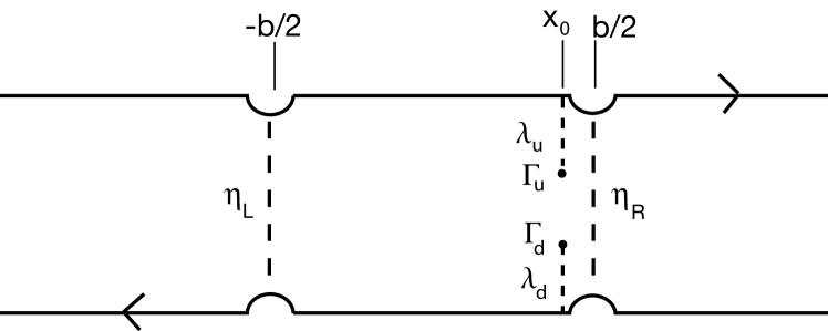
Figure 1: Interferometer with quasi-particle tunneling at positions $-b/2$ and $b/2$. One localized Majorana mode couples to the upper edge at spatial position $x=x_{0}$, another one to the lower edge at the same position. For the derivation of the exact solution, the bulk Majoranas are positioned at the boundary of the interferometer cell with $x_{0}=b/2$.

The neutral parts of the tunneling operators can be expressed as spin fields of an Ising CFT YellowBook

$${\cal N}_{L(R)}\equiv\sigma_{u}(\mp b/2)\sigma_{d}(\mp b/2)\ \ .$$ (10)

The $\sigma$ operators can be defined through their operation on the Majorana fermion fields as SBPRB

$$\psi_{r}(y)\sigma_{r}(x_{0})=\mp{\rm sgn}(x_{0}-y)\sigma_{r}(x_{0})\psi_{r}(y)$$ (11)

with $r=u,d$, and the minus sign going with the upper edge. We will discuss an alternative expression for the neutral tunneling operator in the next paragraph. The factor of $i\Gamma_{u}\Gamma_{d}$ in the second term of Eq. (7) is included to account for the wrapping of a tunneling quasiparticle at position $x=b/2$ around the two localized quasiparticles. This factor is responsible for the $\pi$ phase shift between the interference patterns corresponding to the two eigenvectors of $i\Gamma_{u}\Gamma_{d}$.

The neutral part of the tunneling operator can be expressed in a more intuitive way by using the parity operator for the part of the system to the left of the tunneling site. We arrive at this formulation by representing the 5/2 state as a p-wave superconductor of composite fermions readgreen . In this picture, the quasiparticle with charge $e/4$ is a vortex of the superconductor. The superconducting phase changes by $2\pi$ when encircling the vortex so that the condensate wave function is single valued. As a Cooper pair has two fermions, the phase of the fermionic wave function changes only by $\pi$ when encircling the vortex, and there has to be a branch cut in the phase field seen by unpaired fermions to make their wave function single valued. For this reason, every vortex drags behind it a branch cut in the phase field of unpaired fermions. The phase jump of $\pi$ across the branch cut shows up as the minus sign in the commutation relation Eq. (11): while a Majorana operator at spatial coordinate $y>x_{0}$ is not affected by the tunneling of a charge $e/4$ QP as described by a $\sigma$ operator, for $y<x_{0}$ the Majorana operator acquires an extra minus sign.

Alternatively, the minus sign a Majorana operator acquires when crossing the branch cut left behind by an $e/4$ QP can be described by an operator which shifts the phase of fermions by $\pi$. This operator can be found by using an analogy with spatial translations. A spatial translation by a distance $a$ is described by the exponential $\exp(i\hat{p}a)$, where $\hat{p}$ is the momentum conjugate to the spatial coordinate which is shifted by $a$. In order to describe a ”phase translation”, we need the exponential of the operator conjugate to the phase operator. In a superconductor, phase and number of cooper pairs are conjugate so that the Cooper pair number operator generates phase shifts. At zero temperature, the Cooper pair density is just half the electron density $\hat{\rho}(x)$, and the operator

$$\hat{P}(-\infty,x_{0}) = e^{i\pi\hat{N}(-\infty,x_{0})}$$

$$= e^{i\pi\int_{x<x_{0}}d^{2}r\hat{\rho}(r)}$$

generates a relative phase shift of $\pi$ between operators $\psi(y)$ with $y<x_{0}$ and $y>x_{0}$, respectively. As $\hat{N}(-\infty,x_{0})$ is the fermion number operator for the region $x<x_{0}$, the operator $e^{i\pi\hat{N}(-\infty,x_{0})}$ is just the parity of the number of fermions to the left of $x_{0}$, and we identify the operator $\hat{P}(-\infty,x_{0})$ defined in Eq. (II) as the parity operator. When evaluating $\hat{P}(-\infty,x_{0})\psi_{r}(y)$ for $y<x_{0}$, the change in particle number due to the action of $\psi_{r}(y)$ is included in the evaluation of $\hat{P}(-\infty,x_{0})$ and changes its value by minus one, while for the opposite operator order $\psi_{r}(y)\hat{P}(-\infty,x_{0})$ this is not the case. In this way, Eq. (11) is reproduced for $y<x_{0}$ when making the identification

$$\sigma_{u}(x_{0})\sigma_{d}(x_{0})=\hat{P}(-\infty,x_{0})\ \ .$$ (13)

Clearly, for $y>x_{0}$ the order of $\hat{P}(-\infty,x_{0})$ and $\psi_{r}(y)$ does not influence the value of $\hat{P}(-\infty,x_{0})$, and Eq. (11) is reproduced again.

In the following, it will be useful to decompose the parity operator into a bulk part $\hat{P}_{\rm bulk}$ measuring the parity of bulk Majoranas and an edge part $\hat{P}_{\rm edge}$. In order to keep our model simple, we assume that any localized QPs in the region $x<-b/2$ are far from the edge, so that the occupation number of their associated Majorana states do not change during the course of the experiment. Since the parity operator factorizes according to $\hat{P}_{\rm bulk}(-\infty,b/2)=\hat{P}_{\rm bulk}(-\infty,-b/2)\hat{P}_{\rm bulk}(-b/2,b/2)$, under the above assumption it is sufficient to include only $\hat{P}_{\rm bulk}(-b/2,b/2)$ in the tunneling operator for the right constriction. In our model, there are only two bulk Majoranas $\Gamma_{u}$, $\Gamma_{d}$ inside the interferometer cell with $-b/2<x<b/2$. Their parity is determined by the operator $i\Gamma_{u}\Gamma_{d}$, which indeed appears as a factor in the definition Eq. (7) of the tunneling operator.

As the bulk part of the parity operator is fully described by the factor $i\Gamma_{u}\Gamma_{d}$ in the tunneling Hamiltonian, the neutral operators ${\cal N}_{L,R}$ can be expressed in terms of the edge parity operator. In order to find an explicit expression for it, we express the particle density on upper and lower edge together as $\hat{\rho}_{\rm edge}(x)=i\psi_{u}(x)\psi_{d}(x)$ and find

$$P_{\rm edge}(-\infty,x_{0})=e^{i\pi\int_{-\infty}^{x_{0}}dx\,i\psi_{u}\psi_{d}}\ \ .$$ (14)

As the edge parity operator factorizes in the same way as the bulk parity operator, the equal time neutral correlation function $\langle{\cal N}(-b/2){\cal N}(b/2)\rangle=\langle P_{\rm edge}(-b/2,b/2)\rangle$ is given by the expectation value of the edge parity operator for the interferometer cell

$$P_{\rm edge}(-b/2,b/2)\ =\ e^{i\pi\int_{-b/2}^{b/2}dx\,i\psi_{u}\psi_{d}}\ \ .$$ (15)

This expression will be useful for the treatment of the lattice model introduced in section IV. In the framework of this lattice model, the edge parity operator reduces to a product over local parity operators.

III Signatures of bulk-edge coupling in the interference current

To lowest order in the tunnel couplings $\eta_{L}$, $\eta_{R}$, the expectation value of the interference contribution to the backscattered current can be obtained using linear response theory. In this approach, the perturbation is the tunneling Hamiltonian Eq. (6) and (7). Starting from the relation

$$\langle I\rangle\ =\ {1\over i\hbar}\int_{-\infty}^{0}dt\langle\left[J(0),H_{\rm tun}(t)\right]\rangle\ \ ,$$ (16)

we find after some algebra that the interference contribution to the backscattered current is given by

$$I_{\rm int} = {4e^{\star}\over\hbar^{2}}{\rm Re}\ i\eta_{L}^{\star}\eta_{R}\int_{-\infty}^{\infty}dte^{-ie^{\star}Vt/\hbar}{\rm Im}\Big{[}\langle{\rm T}_{\tau}{\cal C}_{L}^{\dagger}(\tau){\cal C}_{R}(0)\rangle$$ (17)

$$\times\langle{\rm T}_{\tau}{\cal N}_{L}(\tau){\cal N}_{R}(0)i\Gamma_{u}(0)\Gamma_{d}(0)\rangle\Big{]}\Big{|}_{\tau\to it+\delta}\ \ ,$$

where $T_{\tau}$ is the time ordering operator, and $\delta$ is the short time cutoff of the theory. Using the definition Eq. (9), the expectation value of the charged correlator can be directly evaluated as

$$\langle{\rm T}_{\tau}{\cal C}_{L}^{\dagger}(\tau){\cal C}_{R}(0)\rangle = {\delta^{1/4}\over\big{[}\tau^{2}+b^{2}/v_{c}^{2}]^{1/8}}\ \ .$$ (18)

In the absence of bulk-edge coupling, the neutral correlator can be obtained from the representation Eq. (10) by using the the conformal dimension $h_{\sigma}={1\over 16}$ of the $\sigma$-field in the expression for CFT correlation functions YellowBook . One finds

$$\langle{\rm T}_{\tau}{\cal N}_{L}^{\dagger}(\tau){\cal N}_{R}(0)\rangle\Big{|}_{\tau\to it+\delta} = {\delta^{1/4}\over\big{[}\tau^{2}+b^{2}/v_{n}^{2}\big{]}^{1/8}}\ \ .$$ (19)

Alternatively, it can be calculated by using a bosonized version of Eq. (14). Using the lattice model described in the next section, we have been able to obtain an exact solution for the neutral correlation function in the presence of two impurities at $x_{0}={b\over 2}$, one of them coupled to the upper edge and the second coupled to the lower edge. From Eq. (V) we find

$$\langle{\rm T}_{\tau}{\cal N}_{L}^{\dagger}(\tau){\cal N}_{R}(0)i\Gamma_{u}(0)\Gamma_{d}(0)\rangle = {2\delta^{1\over 4}\over\pi v_{n}}\left({b^{2}\over v_{n}^{2}}+\tau^{2}\right)^{3\over 8}$$

$$\times{\lambda_{u}}\left[e^{\lambda_{u}^{2}(b-iv_{n}\tau)/v_{n}^{2}}K_{0}(\lambda_{u}^{2}(b-iv_{n}\tau)/v_{n}^{2})\right]$$

$$\times{\lambda_{d}}\left[e^{\lambda_{d}^{2}(b+iv_{n}\tau)/v_{n}^{2}}K_{0}\left(\lambda_{d}^{2}(b+iv_{n}\tau)/v_{n}^{2}\right)\right]\ ,$$

where $K_{0}(x)$ is the modified Bessel function of order zero. Using this expression in Eq. (17), the interference current can be evaluated for arbitrary system size, bulk edge coupling, and all ratios of $v_{n}/v_{c}$. For illustrative purposes, we evaluate now the interference current in the regime of small interferometer length $b$, in which the interference contrast is highest and where the size $b$ of the interferometer cell can be set to zero. In addition, we will concentrate on a situation with only one impurity present in the bulk, say $\Gamma_{u}$. This situation can be described by sending ${b\lambda_{d}^{2}\over v_{n}^{2}}\to\infty$ in Eq. (LABEL:twoimpneutral.eq) such that the impurity degree of freedom $\Gamma_{d}$ is effectively absorbed by the edge. This situation has the benefit of being more easily interpreted than the two impurity case. We will see that the visibility of the interference signal grows from zero to one as the coupling strength is increased. We define $\omega=-e^{\star}V/\hbar$ and find

$$I_{\rm int} = {4e^{\star}\over\hbar^{2}}{\rm Re}\ i\eta_{L}^{\star}\eta_{R}\sqrt{\delta}\ {\lambda_{u}\over\sqrt{v_{n}}}$$

$$\times\sqrt{2\over\pi}\int_{-\infty}^{\infty}dte^{i\omega t}{\rm Im}\left\{{\sqrt{t-i\delta}\ e^{\lambda_{u}^{2}t/v_{n}}K_{0}\left[{\lambda_{u}^{2}\over v_{n}}(t-i\delta)\right]\over\left[-t^{2}+i\delta\,t\right]^{1\over 4}}\right\}$$

$$= {4e^{\star}\over\hbar^{2}}\sqrt{\delta\pi\over\omega}\ {\rm Re}\left[\eta_{L}^{\star}\eta_{R}J_{\rm imp}\left({\lambda_{u}^{2}\over\omega v_{n}}\right)\right]$$

with

$$J_{\rm imp}(x) = {1\over\sqrt{1+{i\over 2x}}}\ \ .$$ (22)

To evaluate the time integral in Eq. (III), we split the domain of integration into negative and positive times. In each subdomain, the square roots of time in numerator and denominator cancel up to a phase factor so that the integral is a Fourier integral of Bessel functions, which can be found in the literature GraRy . For positive arguments, the Bessel function $K_{0}(x)$ is real, while for negative arguments $x<0$, $K_{0}(x)$ has a cut along the real axis and can be decomposed into real and imaginary part according to $K_{0}(x-i\delta)=K_{0}(-x)+i\pi I_{0}(-x)$.

With respect to the case without bulk impurity, the interference signal is modified by the additional factor $J_{\rm imp}(\lambda_{u}^{2}/\omega v_{n})$ in Eq. (III). The modulus of $J_{\rm imp}$ reduces the amplitude of interference oscillations for small values of $\lambda_{u}^{2}/\omega v_{n}$, while the argument of $J_{\rm imp}$ gives rise to a phase shift. Both modulus and phase of $J_{\rm imp}(x)$ are displayed in Fig. 2.

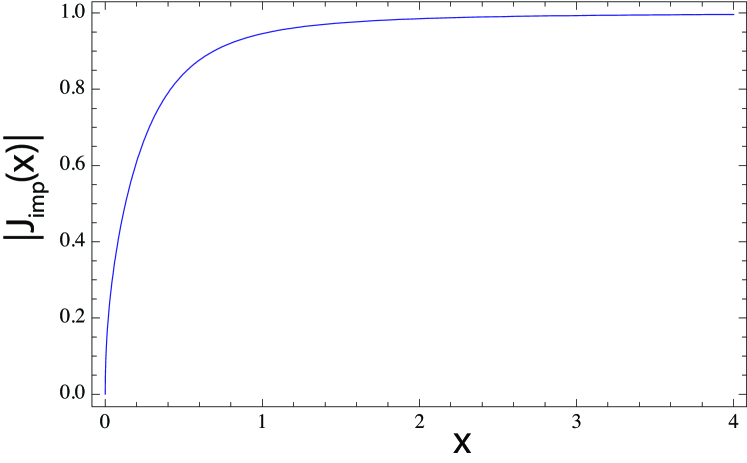
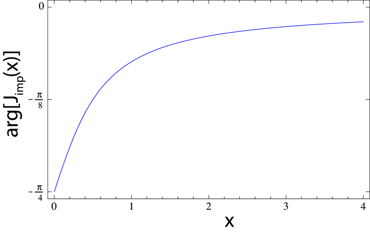
Figure 2: Modulus and argument of the factor $J_{\rm imp}({\lambda^{2}\hbar\over-v_{n}e^{\star}V})$ describing the modification of the interference current due to bulk-edge coupling.

The expansion of $J_{\rm imp}(x)$ for small arguments (weak tunneling or large voltage) is

$$J_{\rm imp}(x)\ =\ (1-i)\sqrt{x}\ +\ (1+i)\ x^{3/2}\ +\ O(x^{5\over 2})\ \ .$$ (23)

The expansion for large arguments (strong coupling expansion) is

$$J_{\rm imp}(x)\ =\ 1\ -\ {i\over 4x}\ -\ {3\over 32x^{2}}\ +\ O\left(x^{-3}\right)\ \ .$$ (24)

Interestingly, bulk edge coupling not only reduces the visibility of interference oscillations but also contributes a phase shift of $\pi/4$ between the weak and strong coupling limit. This universal phase shift as a function of voltage is a signature of bulk-edge coupling in a non-abelian interferometer. The phase $e^{-i\pi/4}$ characteristic of the weak coupling limit can be interpreted as the non-abelian part of the phase acquired by two charge $-e/4$ QHs encircling each other in the clockwise direction. This phase factor agrees with that obtained from the CFT correlation function of two $\sigma$-operators, which describe the non-abelian part of charge $\pm e/4$ particles. Alternatively, the non-abelian phase can be inferred from the fact that non-abelian QHs behave relative to each other as bosons if they are in the I fusion channel, i.e. that abelian and non-abelian part of the phase cancel each otherNaWi96 ; MoRe91 ; TsSi03 . Hence, the non-abelian phase has to compensate the abelian phase $e^{i\pi/4}$ found from the operator product expansion of two $e^{i\varphi(x)/2}$ QH operators.

IV Lattice version of the continuum model

In order to evaluate neutral correlation functions in the presence of bulk-edge coupling beyond perturbation theory, we develop a lattice description of the continuum model introduced in section II. For the lattice model, the parity expectation value can be evaluated numerically for arbitrary strength of bulk edge coupling RoHaSiSt08 , and in section V we will derive the exact solution Eq. (LABEL:twoimpneutral.eq) by using the inversion formula TrSc for so-called Hilbert type matrices. We shall first concentrate on the equal time correlation function

$$\langle{\cal N}_{L}{\cal N}_{R}\rangle\ =\ \langle P_{\rm edge}(-b/2,b/2)\rangle\ \equiv\ \langle P_{b}\rangle\ \ ,$$ (25)

where $P(-b/2,b/2)$ is the edge parity operator for the up and down Majorana modes as defined in Eq. (15). As a first step towards defining a lattice version of this operator, we consider a one-dimensional model of complex lattice fermions defined by the Hamiltonian

$$H_{\rm kin}\ =\ -{v_{n}\over 2a}\sum_{j}\Big{(}c_{j+1}^{\dagger}c_{j}+c_{j}^{\dagger}c_{j+1}\Big{)}\ \ ,$$ (26)

where the sum runs over lattice points $j$, and the lattice constant is denoted by $a$. The kinetic energy describes a dispersion relation

$$\epsilon(k)\ =\ -{v_{n}\over a}\cos k\ ,\ \ \ -{\pi}<k<{\pi}\ \ .$$ (27)

We study the model at half filling with $k_{F}={\pi\over 2}$. Defining $N={b\over a}$, the equal time parity expectation value for the complex lattice fermions is given by

$$\langle e^{i\pi\sum_{j=-N/2}^{N/2}c_{j}^{\dagger}c_{j}}\rangle = \langle\prod_{-{N\over 2}<j<{N\over 2}}(2c^{\dagger}_{j}c_{j}-1)\rangle\ \ .$$ (28)

It is expressed as the expectation value of a product of lattice operators. In order to make contact with a non-abelian 5/2-edge, we define Majorana operators

$$\gamma_{j} = e^{ij\pi/2}\ c_{j}\ +\ e^{-ij\pi/2}\ c_{j}^{\dagger}$$ (29a)

$$\tilde{\gamma}_{j} = {1\over i}\big{(}e^{ij\pi/2}\ c_{j}\ -\ e^{-ij\pi/2}\ c_{j}^{\dagger}\big{)}$$ (29b)

$$i\gamma_{j}\tilde{\gamma}_{j} = 2c_{j}^{\dagger}c_{j}-1\ \ .$$ (29c)

This transformation corresponds to a boost to the right moving Fermi point. The left moving Fermi point now corresponds to the momentum $-\pi$. Using the equality Eq. (29c), the parity expectation value Eq. (28) can be expressed as the expectation value of a product of $\gamma$ and $\tilde{\gamma}$ operators. As the Hamiltonian is quadratic, Wicks’s theorem can be used to evaluate the expectation value of this product as the Pfaffian form of the matrix of correlation functions. The Hamiltonians for the $\gamma$- and $\tilde{\gamma}$-mode are

$${\cal H} = {v_{n}\over 4a}\int_{-\pi}^{\pi}{dk\over 2\pi}\gamma_{-k}\ \sin(k)\;\gamma_{k}\ \ ,$$ (30a)

$$\tilde{\cal H} = {v_{n}\over 4a}\int_{-\pi}^{\pi}{dk\over 2\pi}\tilde{\gamma}_{-k}\ \sin(k)\;\tilde{\gamma}_{k}\ \ .$$ (30b)

As there is no coupling term between the two Majorana modes, the correlation function matrix decomposes into a block with $\gamma$–correlators and another block with $\tilde{\gamma}$–correlators. Although we initially need both modes to write down an expression for the local parity operator, the determinant of the correlation function matrix factorizes and it is sufficient to consider the $\gamma$-Majorana mode only. We can now identify the right-moving branch of $\gamma$ with the upper edge and the left-moving branch with the lower edge.

States with momenta between $-\pi$ and $0$ are occupied, hence the zero temperature correlation function is given by

$$\langle i\gamma_{j}\gamma_{l}\rangle\ =\ 2i\int_{-\pi}^{0}{dk\over 2\pi}\ e^{ik(j-l)}\ ={1\over\pi}\ {\big{[}1-(-1)^{j-l}\big{]}\over j-l}\ \ .$$ (31)

The correlation function vanishes if $j-l$ is even, and is odd under exchange of $j$ and $l$. The parity expectation value for a system of a right moving and a left moving Majorana mode is given by

$$\langle P_{\rm b}\rangle = \langle\prod_{-{N\over 2}<j<{N\over 2}}\big{(}\sqrt{i}\gamma_{j}\big{)}\rangle\ =\ \sqrt{{\rm det}(\langle i\gamma_{j}\gamma_{j^{\prime}}\rangle)}\ \ .$$ (32)

The r.h.s. of Eq. (32) is positive as required because the eigenvalues of the matrix of correlation functions $\langle i\gamma_{j}\gamma_{j^{\prime}}\rangle$ occur in pairs $\pm i\lambda$ with real $\lambda$. When evaluating the determinant for different system sizes numerically, on finds that it decays as $N^{-1/4}$ in agreement with the analytical result obtained by using $\sigma$–correlators in the Ising CFT.

We next want to calculate the influence of localized bulk modes on the parity expectation value. More specifically, we need to calculate the expectation value

$$\langle P_{b,\rm imp}\rangle\ =\ \langle i\Gamma_{u}\Gamma_{d}\prod_{-{N\over 2}<j<{N\over 2}}\big{(}\sqrt{i}\gamma_{j}\big{)}\rangle\ \ .$$ (33)

In order to evaluate this expectation value, we need to know the edge-edge, the impurity-impurity, and the impurity-edge correlation functions in the presence of a coupling between impurities and edge. The lattice version of the bulk-edge coupling Eq. (5) is

$${\cal H}_{\rm scatter}\ =\ \int{dk\over 2\pi}\ f(k)\big{[}i{\lambda_{u}\over\sqrt{a}}\Gamma_{u}\gamma_{k}\ +\ i{\lambda_{d}\over\sqrt{a}}\Gamma_{d}\gamma_{-2k_{F}+k}\big{]}\ \ .$$ (34)

Here, $f(k)=f(-k)$ is unity for momenta $k\ll 1$ and drops rapidly to zero for larger momenta, such that the dispersion relation can be linearized around the two Fermi points. As the Hamiltonian for bulk and edge Majorana states is quadratic, all correlation functions needed for the evaluation of the parity expectation value Eq. (33) can be evaluated exactly. After integrating out the edge Majorana modes, one obtains an effective action for the bulk states

$${\cal S}_{\rm imp}\! = \!{T\over 2}\sum_{\epsilon_{n}}\left[\Gamma_{u}(-\epsilon_{n})\!\left(\!-{i\epsilon_{n}\over 2}+\lambda_{u}^{2}\!\int{dq\over 2\pi}f(q)G_{0}(i\epsilon_{n},q)\!\right)\!\Gamma_{u}(\epsilon_{n})+\Gamma_{d}(-\epsilon_{n})\!\left(\!-{i\epsilon_{n}\over 2}+\lambda_{d}^{2}\!\int{dq\over 2\pi}f(q)G_{0}(i\epsilon_{n},q-2k_{F})\!\right)\!\Gamma_{d}(\epsilon_{n})\!\right]\ \ .$$

Here,

$$G_{0}(i\epsilon_{n},k)\ =\ {2\over i\epsilon_{n}-{v_{n}\over a}\sin(k)}$$ (36)

denotes the edge Green function in the absence of scattering, $\epsilon_{n}=(2n+1)k_{B}T/\hbar$ is a fermionic Matsubara frequency, and $T$ denotes temperature. Although we use a finite temperature formalism here, we will focus on the zero temperature case in the end. As there is no coupling between the bulk Majorana states, the impurity-impurity correlator vanishes $\langle i\Gamma_{u}\Gamma_{d}\rangle\equiv 0$. The correlation functions between impurity and edge operators are given by

$$\langle i\Gamma_{u}(-\epsilon_{l})\gamma_{k}(\epsilon_{l})\rangle = G_{0}(i\epsilon_{l},k)\ f(k)\ {\lambda_{u}\over\sqrt{a}}$$

$$\times\langle\Gamma_{u}(-\epsilon_{l})\Gamma_{u}(\epsilon_{l})\rangle_{{\cal S}_{\rm imp}}\ \ ,$$

$$\langle i\Gamma_{d}(-\epsilon_{l})\gamma_{k}(\epsilon_{l})\rangle = G_{0}(i\epsilon_{l},k-2k_{F})\ f(k)\ {\lambda_{d}\over\sqrt{a}}$$

$$\times\langle\Gamma_{d}(-\epsilon_{l})\Gamma_{d}(\epsilon_{l})\rangle_{{\cal S}_{\rm imp}}\ \ .$$

Due to chirality, the edge-edge correlation function $\langle i\gamma_{l}\gamma_{l^{\prime}}\rangle$ depends on the bulk-edge coupling strengths $\lambda_{d}$, $\lambda_{u}$ only if the coupling to the impurity occurs between the two lattice sites $l$ and $l^{\prime}$. As only edge-edge correlation functions with both $l$ and $l^{\prime}$ inside the interferometer cell are needed for the evaluation of Eq. (33), these edge-edge correlators become independent of the bulk-edge coupling strengths for $x_{0}=b/2$, i.e. for impurities coupling to the boundary of the interferometer cell. In order to simplify the task of calculating the full neutral correlation function including bulk-edge coupling, we will adopt $x_{0}=b/2$ in the following.

In order to extract the universal long distance behavior of correlation functions, we linearize the dispersion relation around the two Fermi points and remove the momentum cutoff when possible. In this way, the Fourier transform $f_{j}$ of a function $f\left[{v_{n}\over a}\sin k\right]$ becomes

$$f_{j} = \int_{-3\pi/2}^{\pi/2}{dk\over 2\pi}e^{ikj}f\left[{v_{n}\over d}\sin k\right]$$ (38)

$$\approx \left(-e^{i\pi j}+1\right)\int_{-\infty}^{\infty}{dk\over 2\pi}f\left[{v_{n}\over d}k\right]e^{ikj}$$

The first term with a rapidly oscillating position dependence is due to integrating over momenta $-3\pi/2<k-\pi/2$, whereas the second term with a smooth position dependence is due to integration over momenta $-\pi/2<k<\pi/2$. With the help of this formula and regularizing momentum integrals as ${i\over\pi}\int_{0}^{\infty}dk\,e^{ik(x+i\eta)}={1\over\pi}{1\over x+i\eta}$, expression Eq. (31) is easily reproduced in the limit $\eta\to 0$. For the bulk-edge correlation functions, one finds

$$\langle i\Gamma_{u}\gamma_{j}\rangle\! = \!{2\lambda_{u}\sqrt{a}\over\pi v_{n}}\;e^{2\lambda_{u}^{2}ja/v_{n}^{2}}E_{1}(2\lambda_{u}^{2}ja/v_{n}^{2})\ \ ,$$ (39)

$$\langle i\Gamma_{d}\gamma_{j}\rangle\! = \!(-1)^{j}\;{2\lambda_{d}\sqrt{a}\over\pi v_{n}}\;e^{2\lambda_{d}^{2}ja/v_{n}^{2}}E_{1}(2\lambda_{d}^{2}ja/v_{n}^{2}).$$ (40)

Here, the exponential integral is defined as

$$E_{1}(x) = \int_{1}^{\infty}dt\;{e^{-tx}\over t}\ \ .$$ (41)

It has the asymptotic expansions

$$E_{1}(x) \to -\gamma-\ln x\ \ \ \ {\rm for}\ \ \ x\to 0\ \ ,$$ (42)

$$E_{1}(x) \to {e^{-x}\over x}\ \ \ \ {\rm for}\ \ \ x\to\infty$$

with $\gamma=0.57721...$ denoting Euler’s constant. Although it is not needed for the calculations presented in this manuscript, we would like to mention the result for the edge-edge correlation function in the presence of bulk-edge coupling, which was used to obtain the numerical result for the reduction factor in Ref. RoHaSiSt08, . It is given by

$$\langle\gamma_{j}\;\gamma_{l}\rangle_{\rm imp} = {1\over\pi}\ {1\over j-l}\ [1-(-1)^{j-l}]$$

$$-{4\lambda_{u}^{2}a\over\pi v_{n}^{2}}\ e^{2\lambda_{u}^{2}(j-l)a/v_{n}^{2}}\ E_{1}\big{[}2\lambda_{u}^{2}(j-l)a/v_{n}^{2}\big{]}\$$

$$\times\left[\Theta(j)\Theta(-l)-\Theta(-j)\Theta(l)\right]$$

$$-(-1)^{j-l}\ {4\lambda_{d}^{2}a\over\pi v_{n}^{2}}\ e^{2\lambda_{d}^{2}(l-j)a/v_{n}^{2}}\ E_{1}\big{[}2\lambda_{d}^{2}(l-j)a/v_{n}^{2}\big{]}\$$

$$\times\left[\Theta(-j)\Theta(l)-\Theta(j)\Theta(-l)\right]\ \ .$$

V Exact solution for parity correlation function with impurities

As explained in the last section, we consider a geometry where the bulk impurity couples to the edge at the boundary of the interferometer cell, i.e. $x_{0}=b/2$. This geometry somewhat simplifies calculations because now the edge-edge correlation function does not have an impurity contribution. For ease of notation, we assume ${a\lambda_{u}^{2}\over v_{n}^{2}}={a\lambda_{d}^{2}\over v_{n}^{2}}\equiv\lambda^{2}$ in the following, the generalization to two different couplings is straightforward.

Again we will be calculating a correlation function by using Wick’s theorem to rewrite that correlation function as a determinant analogous to Eq. (32). However, here we will calculate the more complicated correlation function Eq. (33). We denote the matrix of correlation functions, whose determinant needs to be calculated, by ${\bf\sf C}$. All diagonal elements of ${\bf\sf C}$ vanish. We adopt a bra-ket notation in the following and denote a position along the edge by $|j\rangle$, and the two bulk impurities by $|u\rangle$, $|d\rangle$. The edge-edge correlation function is then given by $\langle j|{\bf\sf C}|j^{\prime}\rangle$, the bulk-edge correlation is

$$\langle j|{\bf\sf C}|u\rangle = {2\lambda\over\pi}e^{2\lambda^{2}j}E_{1}(2\lambda^{2}j)\ \ ,$$

$$\langle j|{\bf\sf C}|d\rangle = (-1)^{j}{2\lambda\over\pi}e^{2\lambda^{2}j}E_{1}(2\lambda^{2}j)\ \ \ .$$ (44)

The impurity-impurity correlation function is $\langle u|{\bf\sf C}|d\rangle=\langle d|{\bf\sf C}|u\rangle\equiv 0$. Our result is again a square root of a determinant, and the determinant is the product of all eigenvalues. Let us assume we know the eigenvalues of the edge-edge part. For small $\lambda$, the bulk-edge correlation functions $\langle j|{\bf\sf C}|u\rangle$, $\langle j|{\bf\sf C}|d\rangle$ are of order $\lambda\ln^{2}\lambda$, and the leading contribution to the determinant is obtained by multiplying the determinant of the edge-edge correlators with the perturbatively calculated eigenvalues of the impurity-impurity part of the matrix. Although the eigenvalues are calculated perturbatively in $\lambda$, which is proportional to the lattice constant and goes to zero in the continuum limit, the final result is valid even in the strong coupling regime with large $\lambda N$. The square root of the product of these two eigenvalues is the reduction factor $R(b)$, i.e. the ratio

$$R\ =\ {\langle{\cal N}_{L}{\cal N}_{R}i\Gamma_{u}\Gamma_{d}\rangle\over\langle{\cal N}_{L}{\cal N}_{R}\rangle_{0}}$$ (45)

of the neutral expectation value in the presence of two impurities to the expectation value without impurities.

Without bulk-edge coupling, C has two zero eigenvalues. To determine the shift of these zero eigenvalues due to the coupling between impurities and edges, we use second order perturbation theory to calculate the effective matrix elements $\langle u|{\bf\sf C}|d\rangle_{\rm eff}$ due to ”virtual transitions” of a bulk Majorana to the edge and back. Up to a sign, the reduction factor is then equal to this effective matrix element,

$$R\ =\ \langle u|{\bf\sf C}|d\rangle_{\rm eff}\ \ .$$ (46)

To calculate the effective matrix element, we change to a new basis

$$|a\rangle=|u\rangle+|d\rangle\ \ ,\ \ \ \ |b\rangle=|u\rangle-|d\rangle\ \ .$$ (47)

In the new basis, $|a\rangle$ only couples to even lattice sites, while $|b\rangle$ only couples to odd ones. To exploit this, it is useful to decompose the lattice into even and odd sites according to

$$j=2n+{1\over 2}(1+\sigma)\ \ ,\ \ \ \ \ j^{\prime}=2n^{\prime}+{1\over 2}(1+\sigma^{\prime})\ \ .$$ (48)

We assume that the number of lattice sites $N$ is even such that this decomposition works. Then, $n$ runs from $0$ to $N/2$, and $\sigma=\pm 1$ determines whether the lattice site is even or odd. In analogy to Eq. (48), we use an $|n\sigma\rangle$ basis in the following, where $|n\sigma\rangle\equiv|j\rangle$ with $j$ given by Eq. (48). Denoting the eigenvectors of the bulk-bulk part C⁰ of C by $|{\bf\sf e}_{l}\rangle$ and the corresponding eigenvalues by $\lambda_{l}$, the effective matrix element between $|a\rangle$ and $|b\rangle$ state is given by

$$\langle b|{\bf\sf C}|a\rangle_{\rm eff} = \sum_{l=1}^{N}{\langle b|{\bf\sf C}|{\bf\sf e}_{l}\rangle\langle{\bf\sf e}_{l}|{\bf\sf C}|a\rangle\over\lambda_{l}}$$

$$= \sum_{j,j^{\prime}}\langle b|{\bf\sf C}|j\rangle\langle j|({\bf\sf C}^{0})^{-1}|j^{\prime}\rangle\langle j^{\prime}|{\bf\sf C}|a\rangle$$

$$= \sum_{nn^{\prime}}\langle b|{\bf\sf C}|n+\rangle\langle n+|({\bf\sf C}^{0})^{-1}|n^{\prime}-\rangle\langle n^{\prime}-|{\bf\sf C}|a\rangle$$

with (see Eq. (40)

$$\langle b|{\bf\sf C}|n+\rangle=\langle n-|{\bf\sf C}|a\rangle={4\lambda\over\pi}e^{4\lambda^{2}n}E_{1}\left(4\lambda^{2}n\right)\ \ .$$ (50)

The physical interpretation of the effective matrix element Eq. (V) is that the $|a\rangle$ bulk state makes a virtual transition to the edge and then back to the $|b\rangle$ state. For this reason, the double sum in the second line of Eq. (V) runs over edge states only. In order to calculate matrix elements of $({\bf\sf C}^{0})^{-1}$, we use the fact that in the $n$, $\sigma$ basis ${\bf\sf C}^{0}$ has the form

$${\bf\sf C}^{0}=\left(\begin{array}[]{cc}{\bf\sf 0}&{\bf\sf D}\\ -{\bf\sf D}^{T}&{\bf\sf 0}\end{array}\right)$$ (53)

with

$$D_{nn^{\prime}}=C^{0}_{nn^{\prime},-+}={2\over\pi}{1\over 2(n-n^{\prime})-1}\ \ ,$$ (54)

see Eq. (31). Then,

$$\langle n+|{\bf\sf C}^{-1}|n^{\prime}-\rangle=\left({\bf\sf D}^{-1}\right)_{nn^{\prime}}\ \ .$$ (55)

Matrices of the form of D are known as Hilbert-type, and using the inversion formula derived by Trench Scheinok TrSc we find that the inverse of D is given by

$$\left({\bf\sf D}^{-1}\right)_{mn} = {\pi\over 4}{1\over n-m-{1\over 2}}\prod_{q\neq m}\left[1-{1\over 2(q-m)}\right]$$ (57)

$$\times\prod_{s\neq n}\left[1-{1\over 2(n-s)}\right]$$

$$= {1\over\pi}{1\over n-m-{1\over 2}}{\Gamma\left({1\over 2}+m\right)\Gamma\left({1\over 2}+{N\over 2}-m\right)\over\Gamma(m)\Gamma\left(1+{N\over 2}-m\right)}$$

$$\times{\Gamma\left(n-{1\over 2}\right)\Gamma\left({3\over 2}+{N\over 2}-n\right)\over\Gamma(n)\Gamma\left(1+{N\over 2}-n\right)}\ \ .$$

As we will finally take the limit $N\to\infty$ with $N\lambda^{2}$ fixed, we can use Sterling’s formula to simplify

$$\left({\bf\sf D}^{-1}\right)_{mn}\approx{1\over\pi}{1\over n-m-{1\over 2}}\sqrt{m\over n}\sqrt{1+{N\over 2}-n\over 1+{N\over 2}-m}\ \ .$$ (58)

As the formula Eq. (V) uses only the symmetric part of D^-1, we symmetrize and obtain

$$\left({\bf\sf D}^{-1}\right)_{{\rm even},mn}=-{N+2\over 4\pi}{1\over\sqrt{mn}\sqrt{(1+{N\over 2}-n)({N\over 2}+1-m}}\ \ .$$ (59)

Taking everything together, the reduction factor is

$$R={N+2\over 4\pi}\left({4\lambda\over\pi}\right)^{2}\left[\sum_{n-1}^{N\over 2}e^{4\lambda^{2}n}E_{1}\left(4\lambda^{2}n\right){1\over\sqrt{n}\sqrt{{N\over 2}+1-n}}\right]^{2}\ .$$ (60)

Taking the continuum limit, one finds

$$R = \lambda^{2}N{2\over\pi^{3}}\left[\int_{0}^{\lambda^{2}N}dxe^{2x}E_{1}\left(2x\right){1\over\sqrt{x(\lambda^{2}N-x)}}\right]^{2}$$ (61)

$$= \lambda^{2}N{2\over\pi}\left[e^{\lambda^{2}N}K_{0}\left(\lambda^{2}N\right)\right]^{2}\ \ .$$

For the evaluation of the integral in the last equation, we used the integral representation Eq. (41) for $E_{1}(x)$ and evaluated the $x$-integral in terms of a modified Bessel function $I_{0}(x)$, for details see Ref. GraRy, . The remaining integral is again tabulated in Ref. GraRy, . One sees that the reduction factor is the square of reduction factors due to the two individual impurities. Using the asymptotic behavior of the zeroth order modified Bessel function $K_{0}(z)\approx-\ln z$ for $z\to 0$ and $K_{0}(z)\approx\sqrt{\pi\over 2z}e^{-z}$ for $z\to\infty$, we find the asymptotic behavior of the reduction factor

$$R(\lambda^{2}N\ll 1) = {2\over\pi}\lambda^{2}N\left(\ln\lambda^{2}N\right)^{2}\ \ ,$$

$$R(\lambda^{2}N\to\infty) = 1\ \ .$$ (62)

Because of the chirality of upper and lower edge, the time dependence of the exact solution can be obtained by replacing $b\to b-i\tau$ in the factor describing the upper edge and $b\to b+i\tau$ in the factor describing the lower edge in Eq. (61) such that the time dependent reduction factor is given by

$$R(b,\tau) = {\lambda_{u}\lambda_{d}\over v_{n}^{2}}\ {2\over\pi}\ \sqrt{b^{2}+v_{n}^{2}\tau^{2}}$$

$$\times\left[e^{\lambda_{d}^{2}(b+iv_{n}\tau)/v_{n}^{2}}K_{0}\left(\lambda_{d}^{2}(b+iv_{n}\tau)/v_{n}^{2}\right)\right]$$

$$\times\left[e^{\lambda^{2}_{u}(b-iv_{n}\tau)/v_{n}^{2}}K_{0}\left(\lambda_{u}^{2}(b-iv_{n}\tau_{/}v_{n}^{2}\right)\right]\ \ .$$

This extension of the static solution to finite time differences can be justified by considering the case of one bulk impurity coupled to one of the edges, say the upper one, first. Then, we define a neutral correlation function

$${\cal N}_{u}(x_{2},\tau_{2};x_{1},\tau_{1};x_{0})\ =\ \langle T_{\tau}\sigma_{u}(x_{2},\tau_{2})\sigma_{u}(x_{1},\tau_{1})\sqrt{i}\Gamma_{u}\rangle\ ,$$ (64)

which in principle could depend on the four arguments $x_{1}$, $x_{2}$, $\tau_{1}$, $\tau_{2}$ and the parameter $x_{0}$ (position of bulk-edge coupling) separately. As the impurity is static, there is translational invariance in time and ${\cal N}_{u}$ can only depend on the difference $\tau_{2}-\tau_{1}$. As we consider a situation where the impurity is coupled to a point inside the cell, we have $x_{2}<x_{0}$. Then, due to chirality, the field $\sigma_{u}(x_{2},\tau_{2})$ is not influenced by bulk-edge coupling and does not depend on $x_{2}$ and $\tau_{2}$ separately but only on the combination $x_{2}+i\tau_{2}$, and it satisfies the differential equation $(\partial_{x_{2}}+i\partial_{\tau_{2}})\sigma_{u}(x_{2},\tau_{2})=0$. If we restrict ourselves to time differences $\tau_{2}-\tau_{1}\neq 0$ different from zero, the correlation function ${\cal N}_{u}$ satisfies the same differential equation and can for this reason only depend on the variables $x_{2}+i(\tau_{2}-\tau_{1})$ and $x_{1}$. However, from Eq. (61) we see that the static correlation function only depends on the difference $x_{1}-x_{2}$, so we can conclude that ${\cal N}_{u}(x_{2},\tau_{2};x_{1},\tau_{1};x_{0})$ is a function of the single variable $x_{1}-x_{2}-i(\tau_{2}-\tau_{1})$, and that the correct analytic continuation of Eq. (61) is indeed given by replacing $b\to b-i\tau$ with $b=x_{1}-x_{2}$ and $\tau=\tau_{2}-\tau_{1}$. The analytic continuation for the lower edge can be derived by a similar argument.

VI Interpretation in terms of resummed perturbation theory

In this section, we show that the exact solution Eq. (61) can be reproduced by resumming the perturbative expansion of the neutral correlation function in powers of the bulk-edge coupling constant. The terms contributing to this resummation are those which turn the zeroth order bulk-bulk correlation function $\langle T_{\tau}\Gamma_{r}(\tau)\Gamma_{r}(0)\rangle_{0}\equiv 1$ into the full correlator. The $\sigma_{u}\sigma_{u}\psi_{u}$-correlation function appearing in the lowest order expression Eq. (66) is not modified in the perturbative expansion due to the special choice $x_{0}=b/2$, which implies that the chiral $\sigma_{u}\sigma_{u}\psi_{u}$-correlation function is only evaluated for spatial arguments $x\leq x_{0}$. As one can see for example from the edge-Majorana correlation function Eq. (IV), bulk-edge coupling is only important if one spatial argument is to the left and another one to the right of $x_{0}$.

Since upper and lower edge decouple in perturbation theory (modulo fusion channels), we consider only one impurity coupled to one edge, say the upper edge. We start by calculating the neutral equal time correlation function

$${\cal I}_{u}\ =\ \langle\sigma_{u}(-b/2)\sigma_{u}(b/2)\sqrt{i}\Gamma_{u}\rangle$$ (65)

in perturbation theory. The lowest order contribution is RoHaSiSt08

$${\cal I}_{u}^{(1)}\! = \!-\sqrt{i}\lambda_{u}\!\int_{-\infty}^{\infty}\!\!\!\!\!d\tau\langle T_{\tau}\sigma_{u}(-{b\over 2},0+)\sigma_{u}({b\over 2},0-)\psi_{u}({b\over 2},\tau)\rangle_{0}$$ (66)

$$\times\langle T_{\tau}\Gamma_{u}(\tau)\Gamma_{u}(0)\rangle_{0}\ \ .$$

This expression is logarithmically divergent and needs to be regularized by a cutoff on the time integral, which in Ref. RoHaSiSt08, was inserted by hand. However, when resumming the infinite set of diagrams which turns the zero order correlator into the full correlator, the integral becomes finite and we are able to reproduce the exact solution for the reduction factor in Eq. (61). In order to verify this proposition, we calculate the expression Eq. (66) with $\langle T_{\tau}\Gamma_{u}(\tau)\Gamma_{u}(0)\rangle_{0}$ replaced by the full correlation function $\langle T_{\tau}\Gamma_{u}(\tau)\Gamma_{u}(0)\rangle$. From the action Eq. (LABEL:S_imp.eq) we find in frequency space

$$-\langle\Gamma_{u}(-\epsilon_{l})\Gamma_{u}(\epsilon_{l})\rangle\ =\ {2\over i\epsilon_{l}+{2i\lambda_{u}^{2}\over v_{n}}{\rm sign}\epsilon_{l}}\ \ .$$ (67)

After calculating the Fourier transform to Matsubara time we find

$$-\langle T_{\tau}\Gamma_{u}(\tau)\Gamma_{u}(0)\rangle={1\over\pi}{\rm Im}\left[e^{-i\tau 2\lambda_{u}^{2}/v_{n}}E_{1}(-i\tau 2\lambda_{u}^{2}/v_{n})\right]\ \ .$$ (68)

The calculation can be expressed in a more compact fashion by defining

$$g(-z)\ =\ {1\over\pi}e^{-2z\lambda_{u}^{2}/v_{n}}E_{1}(-2z\lambda_{u}^{2}/v_{n})\ \ .$$ (69)

In addition, we make use of the CFT correlation function

$$\langle\sigma_{u}(-b/2,0+)\sigma_{u}(b/2,0-)\psi_{u}(b/2,\tau)\rangle_{0} = {1\over\sqrt{2\pi}}\left(-b\right)^{3\over 8}$$ (70)

$$\times{1\over\sqrt{(b+i\tau)i\tau}}\ \ .$$

Note that the additional factor $1/\sqrt{\pi}$ in Eq. (70) as compared to Ref. RoHaSiSt08, is due to the difference in the Majorana Lagrangian Eq. (3) as compared to RoHaSiSt08, . Now we can express the equal time correlation function as

$${\cal I}_{u} = \sqrt{i}\lambda_{u}(-b)^{3\over 8}{1\over\sqrt{2\pi}}\int_{-i\infty}^{i\infty}{dz\over i}\ {g(-z)-g(z)\over\sqrt{z(z+b)}}\ .$$ (71)

We close the integration contour in the right half plane for the integral over $g(z)$ and in the left half plane for $g(-z)$. We are allowed to do so because $g(z)\sim 1/z$ for large $z$ in the right half plane, which together with the asymptotic $1/z$ behavior of the $\langle\sigma\sigma\Psi\rangle$ correlator makes sure that the infinite semicircle does not contribute to the integral. As the $\langle\sigma\sigma\Psi\rangle$ correlator has a cut only along the negative real axis between $z=-b$ and $z=0$, the integral over $g(z)$ vanishes. The integral over $g(-z)$ can be converted into a contour encircling this cut and gives

$${\cal I}_{u} = \lambda_{u}\sqrt{i}(-b)^{3\over 8}\sqrt{2\over\pi^{3}}\int_{0}^{b}dx\ {e^{-2x\lambda_{u}^{2}/v_{n}}E_{1}(2x\lambda_{u}^{2}/v_{n})\over\sqrt{(b-x)x}}\ \ .$$

We note that the expression for ${\cal I}_{d}$ differs from Eq. (LABEL:Iu.eq) by a factor of $i$ due to the opposite chirality in the correlator Eq. (70). For this reason, the reduction factor obtained from the product ${\cal I}_{u}{\cal I}_{d}$ is real in agreement with Eq. (61). The expression Eq. (LABEL:Iu.eq) agrees up to a phase factor with the correlation function obtained from the square root of the reduction factor Eq. (61). As an additional benefit, using the finite temperature expressions for the $\langle\sigma\sigma\Psi\rangle$ and $\langle\Gamma_{u}\Gamma_{u}\rangle$ correlators opens a route towards a generalization to finite temperature.

VII Discussion

In this paper, we have analyzed the influence of a tunnel coupling between bulk and edge Majorana states on the visibility and phase of interference oscillations in a non-abelian $\nu=5/2$ quantum Hall interferometer. Such a tunnel coupling is important because it blurs the distinction between bulk and edge degrees of freedom and thus complicates the observation of the even-odd effect as a signature for non-abelian statistics. In our discussion, we have focused on the behavior at temperature $T=0$, for an interferometer encircling one or two localized quasiparticles (QPs), as a function of the source-drain voltage and the strength of coupling between the Majorana modes of the impurities and the neutral modes of the edge.

The present paper is an extension of results presented in a previous letter by the authors.RoHaSiSt08 In the present paper, we have found an exact analytic formula for the equal-time parity correlation function for the two ends of the interferometer, when the localized quasiparticles are both located close to one end, and we have verified that the correlation function saturates, in the strong coupling limit, at the same value as one would find in the absence of localized quasiparticles. This correlation function was only obtained numerically in our previous work. Analyzing the analytic properties of the function in the space-time plane, we now obtain an analytic form for the correlation function at two different times, and from that we can predict the dependence of the interference amplitude on the applied voltage and the bulk-edge coupling strengths. We have also been able to examine the phase shift in the interference pattern introduced by the presence of a finite coupling between the bulk QPs and the edge. In addition, the current paper presents various details of the analysis that had to be omitted from Ref. RoHaSiSt08, due to lack of space.

In our work, we have particularly examined the case of a short interferometer, or relatively low voltage, where the interference visibility is largest. Specifically, we assume $t_{V}\gg t_{b}$, where, $t_{b}=b/v_{n}$ is the time needed for a neutral excitation to move along one edge, from one constriction the other, and $t_{V}=\hbar/e^{\star}V$ is the extension in time of a QP wave packet transferred from one edge to the other by backscattering at one of the constrictions. We shall summarize here the qualitative results of our studies, and then say a few words about their implications for experiments.

We start by discussing the case of a single bulk Majorana mode inside the interferometer. In the absence of bulk-edge coupling, the leading harmonic of the interference signal vanishes. In agreement with previous analyses of this problem overbosch07 ; RoHaSiSt08 , we find that for weak coupling, at $T=0$, interference can be observed but is reduced by a factor proportional to $\sqrt{t_{V}/t_{\lambda}}$, where $t_{\lambda}=(\pi\lambda^{2}/2v_{n})^{-1}$ is the characteristic tunneling time associated with the exchange of a Majorana particle between the localized QP and the edge. For large values of the effective coupling constant $t_{V}/t_{\lambda}$, the bulk Majorana mode is effectively absorbed by the edge and the interference signal is fully restored, such that the strong coupling case corresponds to an interferometer with no bulk degree of freedom. In addition, on the way from weak to strong coupling, the phase of the interference signal is shifted by $\pi/4$. Although bulk-edge coupling enforces a modification of the way one looks at the even-odd effect, it actually enriches this effect with a new direction in parameter space, as the dimensionless coupling strength $t_{V}/t_{\lambda}$ depends on source drain voltage. The signature for an odd number of impurities, with just one of them coupled to the edge, is not the complete absence of the leading harmonic, but rather a reduced amplitude, which depends on the applied voltage. The interference intensity grows with decreasing voltage at a rate which is enhanced relative to the behavior in the absence of a bulk Majorana mode (the intensity grows $\propto 1/V$ instead of $\propto 1/\sqrt{V}$ ) until the reduction factor saturates at unity. In addition, when the reduction factor is small compared to unity, the interference factor will have universal phase shift of $\pi/4$ relative to the pattern in the strongly coupled regime.

Our results for a single bulk QP at $T=0$ can be readily generalized to the case of finite temperatures. Qualitatively, the temperature will make relatively little difference as long as $kT$ is small compared to $e^{*}V$. However in the opposite limit, temperature will be important, and its effect may be roughly estimated by replacing the the voltage time $t_{V}$, in the formulas above, by the thermal time $t_{T}\equiv\hbar/kT$. A more quantitative analysis can be given, but it will not be discussed here.

In the case of two bulk Majorana modes coupled to opposite edges, with comparable coupling strengths, the average value of the interference signal shows the same qualitative behavior as in the case of a single impurity. However, the average value of the interference current now has a more subtle interpretation than in the case of a single impurity: due to the presence of the factor $i\Gamma_{u}\Gamma_{d}$ in the tunneling operator, the interference signal is sensitive to the state of the two bulk Majorana modes even in the absence of bulk-edge coupling. Although in the absence of bulk-edge coupling the expectation value of $i\Gamma_{u}\Gamma_{d}$ does not change in time once it is prepared in an eigenstate, the quantum statistical average $\langle i\Gamma_{u}\Gamma_{d}\rangle$ is zero, as the average is taken over both possible states of the system. Experimentally, then, the quantum statistical average corresponds to a situation where the interference signal is averaged over different initializations of the bulk states.

In the presence of weak but non-zero coupling between the bulk and edge modes, two things happen: i) the quantum mechanical average $\langle i\Gamma_{u}\Gamma_{d}\rangle\propto(t_{v}/t_{\lambda})\ln^{2}[t_{\lambda}/t_{V}]$ is now finite; and ii) for a single experiment starting with the bulk states initialized in an eigenstate of $i\Gamma_{u}\Gamma_{d}$, the interference phase will fluctuate on the time scale $\min(t_{\lambda u},t_{\lambda d})$, so that the time average of the interference current over these quantum mechanical fluctuations is equal to the quantum statistical average.

Now we must distinguish between two experimental situations. If the experimental measurement is averaged over a time $t_{\rm{av}}$ that is long compared to one or both of the switching times $t_{\lambda}$, then the experiment will measure the statistical average interference signal, which will be very close to zero if $t_{\lambda}$ is much longer than $t_{V}$ and $t_{T}$. On the other hand, if the bulk modes are so weakly coupled to the edge that for both bulk QPs, $t_{\lambda}>t_{\rm{av}}$, then the experiment will not measure a statistical average, but will see only one or the other of two possible fermion states. In this case one will see a full interference signal, with the same amplitude as if the impurities were not there at all, but with a phase that depends on the starting configuration of the system.

More generally, we may distinguish three ranges of coupling strengths for a QP localized in the bulk. If coupling to the edge is so weak that $t_{\lambda}>t_{\rm{av}}$, we may say that the bulk state is “decoupled” from the edge. If the coupling is in the range where $t_{\lambda}$ is small compared to $t_{V}$ and $t_{T}$, then QP is “strongly coupled” to the edge. If the coupling strength is in the range where $t_{\lambda}$ is small compared to $t_{\rm{av}}$, but large compared to either $t_{V}$ or $t_{T}$, then we may say that the QP is “weakly coupled” to edge.

In an experiment where the interfering edge encloses two or more localized QPs, we may ignore any strongly coupled QPs, as they will be effectively incorporated into the edge. If there are no “weakly coupled” QPs inside the loop, then the presence or absence of the interference signal corresponding to charge e/4 will be determined by the number of decoupled QPs inside the loop. The interference pattern will be present if this number is even, and absent otherwise. If there are any weakly coupled QPs inside the loop, however, with relaxation time $t_{\lambda}$ small compared to the experimental averaging time, then the interference pattern will be absent, regardless of the number of decoupled QPs that may also be present.

In a recent experiment by Willett et al. Willett08 , resistance oscillations in a Fabry-Perot device were studied experimentally. For magnetic fields near a bulk filling fraction $\nu=5/2$, oscillations in the longitudinal resistance were observed as a function of side gate voltage. Depending on the range over which the side gate voltage was varied, consecutive doubling and halving of the voltage period of resistance oscillations was observed. The side gate voltage was interpreted as changing the area of the interferometer cell. If the bulk filling fraction deviates slightly from the exact value of $5/2$, a change of area will once in a while change the number of QPs inside the interferometer cell by one. If the number of QPs changes from even to odd, the fundamental harmonic is suppressed and the period of the interference signal is halved, while for a change from an odd to an even number of localized QPs inside the cell, the period is doubled. A reduced voltage period in the presence of an odd number of localized QPs can arise from interference of abelian charge $\pm e/2$ QPs or from non-abelian charge $\pm e/4$ QPs encircling the interferometer cell twice. This interpretation of the experiment Willett08 is discussed in more detail in Ref. Qguys09, .

A difficulty with this interpretation is that it seems to require that all QPs inside the edge are either completely decoupled from the edge, or strongly coupled so that they are incorporated into the edge. If there any QPs in the intermediate weakly coupled range, where the Majorana state changes back and forth many times during the averaging time of the experiment, then the interference corresponding to charge e/4 would be completely absent, or at least greatly reduced in size. It is not clear to us, why there should be no weakly coupled QPs inside the interferometer in the interference experiments of Ref. Willett08, , nor is it clear why one should be rid of their effects if such QPs are present. We do note, however, that one possible ingredient that is missing from our analysis is a tunnel coupling that allows for an exchange of Majorana fermions between bulk quasi-particles. In the presence of such a coupling, the degeneracy of the localized bulk Majorana states is removed. The resulting spectrum is then composed of several states. Each of these states corresponds to an interference pattern, whose amplitude and phase are determined by the expectation value and fluctuations of the parity operator in that state. The coupling of the bulk states to the propagating Majorana mode of the edge introduces a width to these states, equilibrates them to the temperature of the edge, and thermally averages the interference pattern. Then, if the splitting between the bulk states is large compared to their width and to the temperature, a well defined interference pattern will be observed. A recent estimate Baraban+09 for the tunnel splitting between quasi-particles is rather sizeable, about $100mK$ for a separation of $0.1$ micron. This effect and the overall problem clearly require further investigation.

Altogether, the experimental results obtained so far are not yet well understood by theory, and it is not yet clear that the observed effects originate from the unique properties of non-abelian quasi-particles at $\nu=5/2$. It is possible that a clue to that question may be obtained from the transition region between two different periods, when a change in the number of localized QPs happens due to a change in area of the interferometer cell, and when the distance between edge and bulk QP decreases as a function of side gate voltage. Then, the bulk-edge coupling should change from small to large values, and one can expect that the theory developed in this manuscript is applicable. It would be interesting to analyze the data of Ref. Willett08, from the point of view of bulk-edge coupling, and to test the theoretical prediction that in the transition region between different gate voltage periods the interference current has a modified power law dependence on source-drain voltage and that there is a $\pi/4$ phase shift as a function of source-drain voltage.

Acknowledgments: After completion of this work we learned that a similar problem was solved by W. Bishara and C. Nayak using a different method BiNa09 . We would like to thank W. Bishara and C. Nayak for interesting discussions and for sharing unpublished results with us. We are indebted to V. Gritsev for leading us to Ref. TrSc, . This work was supported in part by the Heisenberg program of DFG, by NSF grant DMR 0541988, by a grant from the Microsoft Corporation, by the US-Israel Binational Science Foundation, and the Minerva foundation.

References

- (1) C. Nayak, S. H. Simon, and A. Stern, , M. Freedman, and S. Das Sarma, Rev. Mod. Phys. 80, 1083 (2008).
- (2) A. Stern, Annals of Physics 323, 204 (2008) .
- (3) S. Das Sarma, M. Freedman, C. Nayak, Phys. Rev. Lett. 94, 166802 (2005).
- (4) A. Stern and B. I. Halperin, Phys. Rev. Lett. 96, 016802 (2006).
- (5) P. Bonderson, A. Kitaev, and K. Shtengel, Phys. Rev. Lett. 96, 016803 (2006).
- (6) N. Read and D. Green, Phys. Rev. B 61, 10267 (2000).
- (7) C. Nayak and F. Wilczek, Nucl. Phys. B 479, 529 (1996).
- (8) E. Grosfeld, S.H. Simon, and A. Stern, Phys. Rev. Lett. 96, 226803 (2006).
- (9) B. J. Overbosch and X.-G. Wen, arXiv:0706.4339.
- (10) B. Rosenow, B.I. Halperin, S.H. Simon, and A. Stern, Phys. Rev. Lett. 100, 226803 (2008).
- (11) E. Fradkin, C. Nayak, A. Tsvelik, and F. Wilczek, Nucl. Phys. B516, 704 (1998).
- (12) W. Bishara and C. Nayak, Phys. Rev. B 77, 165302 (2008).
- (13) C. de C. Chamon, et al., Phys. Rev. B 55, 2331 (1997).
- (14) P. Fendley, M.P.A. Fisher, and C. Nayak, Phys. Rev. B 75, 045317 (2007).
- (15) See, for example, Conformal Field Theory, P. Di Francesco, P. Mathieu, and D. Sénéchal, Springer-Verlag (1997).
- (16) I.S. Gradstein and I.M. Ryshik, Tables of integrals, series, and products, 6th edition, Academic Press (2000).
- (17) Y. Tserkovnyak and S.H. Simon, Phys. Rev. Lett. 90, 016802 (2003).
- (18) G. Moore and N. Read, Nucl. Phys. B 360, 362 (1991).
- (19) W.F. Trench and P.A. Scheinok, SIAM Review, 8, 57 (1966).
- (20) R.L. Willett, L.N. Pfeiffer, K.W. West, arXiv:0807.0221 (2008).
- (21) W. Bishara, P. Bonderson, C. Nayak, K. Shtengel, J.K. Slingerland, arXiv:0903.3108 (2009).
- (22) M. Baraban, G. Zikos, N. Bonesteel, and S.H. Simon, arXiv:0901.3502 (2009).
- (23) W. Bishara and C. Nayak, arXiv:0906.0327 (2009); talk by C. Nayak at conference New Directions in Low-Dimensional Electron Systems, KITP Santa Barabara (2009), http://online.itp.ucsb.edu/online/lowdim_c09/nayak/oh/24.html