Abstract

In this paper, we study the problem of processing continuous range queries in a hierarchical wireless sensor network. Recently, as the size of sensor networks increases due to the growth of ubiquitous computing environments and wireless networks, building wireless sensor networks in a hierarchical configuration is put forth as a practical approach. Contrasted with the traditional approach of building networks in a “flat” structure using sensor devices of the same capability, the hierarchical approach deploys devices of higher capability in a higher tier, i.e., a tier closer to the server. While query processing in flat sensor networks has been widely studied, the study on query processing in hierarchical sensor networks has been inadequate. In wireless sensor networks, the main costs that should be considered are the energy for sending data and the storage for storing queries. There is a trade-off between these two costs. Based on this, we first propose a progressive processing method that effectively processes a large number of continuous range queries in hierarchical sensor networks. The proposed method uses the query merging technique proposed by Xiang et al. as the basis and additionally considers the trade-off between the two costs. More specifically, it works toward reducing the storage cost at lower-tier nodes by merging more queries, and toward reducing the energy cost at higher-tier nodes by merging fewer queries (thereby reducing “false alarms”). We then present how to build a hierarchical sensor network that is optimal with respect to the weighted sum of the two costs. It allows for a cost-based systematic control of the trade-off based on the relative importance between the storage and energy in a given network environment and application. Experimental results show that the proposed method achieves a near-optimal control between the storage and energy and reduces the cost by $0.989~{}\sim~{}84.995$ times compared with the cost achieved using the flat (i.e., non-hierarchical) setup as in the work by Xiang et al.

1 Introduction

As the computing environment evolves toward ubiquitous computing, there has been increasing attention and research on sensor networks. In the sensor networks environment, sensor nodes are connected through the network to the server (or base station) which collects data sensed at the nodes[1]. Example applications in such an environment include environment monitoring(e.g., temperature, humidity), manufacturing process tracking, traffic monitoring, and intrusion detection in a surveillance system.

In particular, as wireless network becomes more common, there has been a lot of research on wireless sensor networks in which sensor nodes are connected in an ad-hoc network configuration in order to reduce the cost of deployment. In general, the objective in a wireless sensor network is to deploy cheap sensor nodes with limited resources (e.g., battery power, storage space) effectively and to collect data from those sensor nodes by using their limited resources efficiently [8].

There is an increasing trend lately toward large-scale wireless sensor networks[12, 13], as the scope of applications extends to municipality management, global environmental monitoring, etc. These networks typically aim at supporting a large number of sensor nodes deployed in a large area for use by a large number of users. For example, in the Network for Observation of Volcanic and Atmospheric Change (NOVAC) project[11], a wireless sensor networks deployed in 15 volcanoes spread across five continents are connected in a multi-tier configuration to support a global volcano monitoring project. As another example, the EarthNet Online[3] collects earth observation information such as the worldwide weather and bird migrations through wireless sensor networks and makes the information available for thousands of individuals or organizations. This kind of scale upgrade will bring about a proportionate increase of the number of concurrent queries and the amount of sensor data. Thus, we expect an increasing importance of processing a large number of queries and a high volume data effectively in wireless sensor networks. In addition, we expect that building such large scale wireless sensor networks economically is important as well.

With these regards, in this paper, we consider storage requirement needed to store queries in sensor nodes and energy consumption (i.e., battery capacity) needed to send the collected data from those nodes to the server. There exists a trade-off between these two cost factors. Let us explain this trade-off with the centralized approach and the distributed approach[15], which are the two naive approaches to build wireless sensor networks. In the centralized approach, the sensor nodes do not store any query and simply send all data to the server, which then processes all the queries on the data received. In this case, there is no storage cost to store queries in individual sensor nodes but the energy cost is very high. In the distributed approach, on the other hand, individual sensor nodes store all the queries and send only the results of processing the queries to the server, which then simply collects the received query results (This scheme is known as in-network query processing[21]). In this case, the energy cost can be reduced but the storage cost is high.

Neither of these two approaches is suitable for building large scale sensor networks. In the centralized approach, since data are accumulated over the course of being relayed toward the server, sensor nodes near the server should send more data than the nodes farther from the server. As the number of nodes increases, this phenomenon will become more serious. In other words, sensor nodes closer to the server consume more energy than other nodes farther from the server – for sending not only the data generated by themselves but also the data received from other nodes; as a result, those nodes will be burnt out within a short time. Thus, the centralized approach is not appropriate for large scale sensor networks. On the other hand, the distributed approach becomes infeasible as the number of queries increases. A sensor node is not able to process a large number of queries due to the limitation on its memory and computing power. Consider as an example inexpensive Micamotes[13], which typically have only 8$\sim$128 Kbyte flash memory and 0.5$\sim$8 Kbyte RAM. Suppose a mote has 64Kbyte flash memory and 10% of it is available for storing two-dimensional range queries. Additionally, suppose that each attribute value of a query is a real number of four bytes long and that the selection condition of a query is expressed as $c_{1}$ $op_{1}$ A $op_{2}$ $c_{2}$ (A: attribute name; $c_{1}$ and $c_{2}$: attribute values; $op_{1}$ and $op_{2}$: binary comparison operators). Then, the size of one query is at least 16 bytes[8]. and, thus at most 400 queries can be stored in one mote. Obviously, these motes are far too short to store thousands of queries expected of large scale networks. Upgrading the sensor nodes to those with large enough memory will raise the expense, which is not acceptable when there are so many sensor nodes to be deployed.

Recently, in order to overcome these large scale problems, building wireless sensor networks in a hierarchical configuration is considered a practical alternative. A hierarchical wireless sensor network is organized in a multi-tier architecture[2] configured with sensor nodes having different amounts of resources and computation power. Nodes closer to the server have more resources and computation power than those farther from the server, and this makes it possible to carry out the processing that cannot be done with low-capacity nodes only. In hierarchical wireless sensor networks, nodes with smaller resources and computing power are recursively connected to nodes with more resources and computing power[14, 16, 2]; thus, nodes near the server are capable of handling the larger amount of data accumulated from lower tiers. We think this configuration is suitable for resolving the query processing problem in large-scale networks mentioned above. Currently, however, the main stream of research on wireless sensor network query processing is for flat sensor networks (i.e., sensor networks that consist of nodes with the same capability). Accordingly, research on query processing for hierarchical sensor networks has been less than adequate.

This paper proposes a method for building large scale hierarchical sensor networks to process queries effectively with respect to the trade-off between the energy cost and the storage cost. The queries considered in this paper are continuous range queries. Range queries are an important query type in many sensor network applications, particularly in monitoring applications[8], and there has been active research done to improve range query processing performance[6]. The method proposed in this paper is based on the technique of systematically controlling the trade-off between the energy cost and the storage cost through controlled merging of queries with similar ranges. There are existing methods proposed to reduce the energy cost by merging queries to avoid duplicate transmission of query results[10, 19, 20]. They, however, all focus on flat sensor networks and, therefore, cannot utilize the characteristics of hierarchical sensor networks in which nodes at different tiers have different capabilities. Besides, their work does not reflect anything about the trade-off because they do not consider the storage cost at all. In contrast, in this paper, we fully utilize the characteristics by employing a progressive approach, which merges increasingly more queries as the tier goes from the server toward the lowest tier and, in this way, finds the optimal merging at each tier in consideration for the trade-off. More specifically, at lower tier nodes, which are larger in number, the approach works toward reducing the storage requirement by reducing the number of queries through more aggressive merging; in contrast, at higher tier nodes, which are smaller in number, the approach works toward storing more queries through less aggressive merging and, in return, reducing the energy consumption by increasing the query accuracy by filtering out more unnecessary data.

In this paper, we first propose the model and algorithms of the progressive query processing method. This method has two phases: query merging and query processing. The key idea in the query merging phase is to merge queries progressively as the tier goes from the highest (i.e., the server) to the lowest. In other words, it merges the input queries to recursively generate queries to be stored at the next tier nodes, first merging the input queries to generate queries for the second tier nodes, and then merging them to generate the ones for the third tier nodes, and so on. We say that the queries thus stored at multiple tiers form the inverted hierarchical query structure as a whole.

The Inverted hierarchical query structure is a new structure proposed in this paper. It is built from a multi-dimensional index storing the query ranges, by partitioning the index into multiple levels and then storing the root level of the index at the lowest-tier sensor nodes and the leaf level of the index in the server. This structure is based on the characteristics of hierarchical sensor networks that sensor nodes at a higher level store more detailed information while sensor nodes at a lower level store more abstract information. Thus, the structure is an inverse of a general tree-like index structure.

In the query processing phase, the queries are processed progressively, that is, by refining the query result to be more accurate as data are sent from a lower tier to a higher tier. For this, the inverted hierarchical query structure is used to retrieve the query result at each tier.

Next, we propose a method that builds an optimal hierarchical sensor network by systematically controlling the trade-off between the storage cost and the energy cost according to their weights. Since the relative importance between the two costs may vary depending on the application and environment, we formulate the cost of building the network as a weighted sum of the two costs and minimize the total cost. As the optimization target parameter, we use the optimal merge rate – the average rate of merging queries at each tier.

Finally, we show through experiments that the proposed method is useful for building a hierarchical sensor network in a cost effective manner. Specifically, first we show that there is little difference between the optimal merge rate obtained from an analytic model and the rate obtained from experiments; second, we show the superiority of the proposed method over the existing query processing method for flat sensor networks in terms of the total cost.

The rest of this paper is organized as follows. Section 2 discusses related work. Section 3 describes the model and the algorithms of the proposed progressive processing method for hierarchical sensor networks. Section 4 proposes an analytical method for effectively building a hierarchical sensor network. Section 5 shows the superiority of the proposed method over the existing method through experiments. Section 6 concludes the paper.

2 Related Work

In this section, we review the existing research on the continuous range query processing in sensor networks and the state of the art in the hierarchical wireless sensor networks.

2.1 Continuous range query processing in sensor networks

In sensor networks, range query processing can be classified into single range query processing and multiple range query processing. Single range query processing executes only one range query in a system. Multiple range query processing concurrently executes many range queries in a system.

Single continuous range query processing

Li et al. [6] apply the data-centric storage to continuous single query processing. The query processing using the data-centric storage runs as follows. For storing data, each sensor node sends collected data to sensor nodes, where the target sensor nodes are determined by the value of the data element. For processing queries, the server sends a query to only those sensor nodes that have the result data of the query. In the same work, Li et al. study an index structure using an order-preserving hash function for distributing data. That is, nodes that are physically adjacent have the adjacent value ranges of data stored in the nodes.As a result, the method reduces the query processing cost by reducing the average number of hops for sending queries and query results. Madden et al.[8] consider storing data in local sensors (unlike the data-centric approach) and propose building an R-tree-like index (called SRTree) based on the range of sensing values. Both of these works focus on single query processing. Hence, they are not applicable for recent query processing environments that register many queries and process them concurrently.

Multiple continuous range query processing

Ratnasamy et al. [15] propose two basic query processing approaches for multiple query processing in wireless sensor networks. One approach processes queries at the server(called the centralized approach), and the other approach processes queries at the sensor node(called the distributed approach). In the former approach, all queries are stored in the server, and the sensor nodes send all sensed data to the server for query processing. This approach is effective only if the size of the region equivalent to the union of all query regions is close to the size of the entire domain space and, otherwise, incurs the overhead of sending unnecessary data to the server. This approach can reduce the memory requirement of the sensor nodes because it does not store any query in them, but has the disadvantage of incurring significant energy consumption because all data must be sent to the server. In the latter approach, each sensor node stores all queries disseminated from the server and sends to the server only the result of processing the sensor data. Thus, this approach may not have the problem of the former approach, but has the disadvantage that the sensor nodes may not be able to store all queries due to insufficient memory if the number of queries is large. From these two basic query processing approaches, we can observe that there is a trade-off between the memory and the energy which are two important resources of sensor nodes.

Furthermore, recently, there has been research to complement the centralized approach and the distributed approach. Specifically, the proposed methods are to share query processing in an overlapping region in case there are overlapping query conditions. By identifying the overlapping regions among the user queries and rewriting the queries accordingly, the proposed methods eliminate duplicate processing and duplicate data transmission. These methods can be classified into the partitioning method and the merging method.

In the partitioning method, the server partitions the individual query regions into overlapping regions and non-overlapping regions. Then, it sends the partitioned regions and the original queries to sensor nodes, which store them. Query processing is done for each partitioned region, and the query results are merged in the server or sensor nodes. Trigoni et al. [18] and Yu et al. [22] use this method to process range queries on the location information of sensor nodes. This method has the advantage that the result of merging the results of processing each partition is the same as the result of processing the original queries and, therefore, no “false alarm” will happen. It, however, has the disadvantage that, if there are a large number of overlapping query conditions, then the number of partitions to be stored in certain sensor nodes increases and, thus, the necessary storage increases as well.

In the merging method, the server merges the regions of overlapping queries into one merged query region. The server then sends the merged queries to the sensor nodes that store them. Query processing results are then “reorganized” into those of the original queries in the server or sensor node. This method has the advantage that it can process a large number of queries at the same time by reducing the number of queries stored in a sensor node. It, however, has the disadvantage that a “false alarm” may happen as a result of merging queries. Muller and Alonso[10] propose a method that compares the predicates of the range queries to extract those common to all queries and generates one query that has only the common predicates as the query condition. In this method, if there is no predicate common to all queries, then one query with no query condition is generated and, thus, has the problem of incurring a lot of false alarms in that case. Xiang et al. [19, 20] propose a method which incrementally merges overlapping query regions and processes the resulting merged queries instead of the original queries. Here, the incremental merging is done until the cost of sending the false alarms occurring when queries are merged is no larger than the cost of sending duplicate results of overlapping query regions when queries are not merged. Xiang et al.’s query processing method has the meaning of a hybrid approach (i.e., reducing the needed memory amount and the data transmission amount) taking advantage of both the centralized approach and the distributed approach, but targets “flat” sensor networks in which all sensor nodes in the network have the same capability and store the same set of merged queries. Thus, this method has the problem that it cannot utilize the characteristics of hierarchical sensor networks. Our method in this paper basically uses the same query merging method as Xiang et al.’s, but enhances it to control the rate of merging queries depending on the capabilities of individual nodes and to build a hierarchical sensor network. Our method has the advantage that it allows for a systematic control of the trade-off between the memory amount needed and the amount of data sent.

2.2 Hierarchical wireless sensor networks

As the scale of sensor networks increases, the hierarchical structure is used more in real applications than the flat structure in which all sensor nodes have the same capability[2].

Representative examples of such hierarchical wireless sensor networks are PASTA(Power Aware Sensing, Tracking and Analysis)[16] mentioned in COSMOS[16] and SOHAN[4]. PASTA is used in military applications for enemy movement surveillance and is configured with the server and about 400 intermediate tier nodes each clustering about 20 sensor nodes. SOHAN is used in traffic congestion monitoring applications to measure the traffic volume using roadside sensor nodes and is configured with the server and about 50 intermediate tier nodes each clustering about 200 sensor nodes.

We expect that hierarchical sensor networks will be increasingly more utilized in the future as the scale and the requirement of applications increase. However, there has not been any research done on processing multiple queries talking advantage of the characteristics that sensor nodes at different tiers have different capabilities. Srivastava et al. [17] investigated how and on which node to process each operation during query processing in a hierarchical sensor network. This research, however, mainly deals with single query processing and, thus, is difficult to apply to multiple query processing. In this paper, we propose a method for processing multiple queries effectively by utilizing the characteristics of hierarchical sensor networks, i.e., the multi-tier structure made of sensor nodes with different resources and computing power.

3 Progressive processing in hierarchical wireless sensor networks

In this section, we present the progressive processing model and algorithms in hierarchical (i.e., multi-tier) wireless sensor networks.

3.1 Overview

In progressive processing, we systematically control the total processing cost by having the larger number of lower-capacity nodes (at lower tiers) partially process queries and the smaller number of higher-capacity nodes (at higher tiers) process the remainder.

Example 1 (Progressive processing in hierarchical wireless sensor networks): Figure  1(a) shows an example of a hierarchical sensor network organized in three tiers. The nodes at the third (i.e., lowest) tier are the largest in number but the smallest in capability and are connected to the more capable nodes at the second tier. All nodes except the server generate data (i.e., partial query results) periodically and send them to the server relayed via the nodes at higher tiers. The server then provides the final query result to the user. Figure  1(b) shows the set of queries stored in the nodes at each tier at the end of the query merging phase. In this figure, the rectangular regions represent range queries, and the boundary rectangle represents the domain space defined by the attributes specified in the queries. The server stores six original queries, the second tier nodes store three queries resulting from the merge of the six original queries, and the third tier stores two queries resulting from further merging them. In the query processing phase, sensor nodes at the lowest tier process the two queries on the sensed data and send to the second tier only the data satisfying the conditions (i.e., ranges) of the two queries. Then, the sensor nodes at the second tier process the three queries on the data sent from nodes at the lower tier and the data they generate on their own, and send to the server only the data satisfying the query conditions. Since nodes at a higher tier have queries of finer granularity, they can reduce ”false alarms” and thereby reduce energy consumption. The server processes the original queries on the data sent from all nodes at lower tiers and provides the final result to the user.

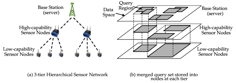
This figure shows a three-tier network as an example.

Figure 1: Inverted hierarchical query structure in a hierarchical wireless sensor network.

From Figure 1(b), we can see that the stored queries altogether form an inverted structure of a multi-dimensional index tree. In contrast to a multi-dimensional index tree structure in which all objects are stored in the leaf nodes and are merged to become more abstract at a higher level, in the proposed structure, the root (i.e., server) stores all objects (i.e., queries) and they are merged to become more abstract at a lower level.

The progressive processing has the query merging phase which generates queries to be stored at each tier of the hierarchical sensor network to form an inverted hierarchical query structure and the query processing phase which processes sensed data and sends the result to the server using the inverted hierarchical query structure. Query merging is performed off-line in batch processing, and query processing is performed on-line every time data are generated. In query merging, queries are sent toward the lowest tier while merged “progressively”, and, in query processing, the sensor data are sent toward the server while being filtered “progressively”.

In the query merging phase, minimum bounding rectangles (MBRs) are obtained from the queries and expressed as merged queries. In this case, it is important to decide how many MBRs the queries should be merged into because the number of MBRs affects the trade-off between the energy consumption and the storage usage. That is, if more queries are merged, then the storage space used by the sensor nodes to store queries is reduced, but the energy consumption is increased due to more frequent false alarms. In this section, we present the model and algorithms under the assumption that the number of merged queries is known at each tier. Then, in section 4, we present a method for determining the optimal number of merged queries analytically using a cost model.

In the query processing phase, all sensor nodes except the server process their own sensed data and the data received from the nodes at lower tiers, and send the results to the nodes at the next higher tier. Since more queries (of finer granularity) are stored at the higher tier nodes, the accuracy of query result is higher in them, thus generating the query result progressively.

3.2 Network and data models

In this section, we first define the hierarchical sensor network. Then, we explain data and queries used in this paper.

The hierarchical sensor network

We make the following assumption about the configuration of a hierarchical sensor network. All sensor nodes are connected to form a tree rooted at the server, and the nodes at the same depth make one tier. Data are generated by not only the nodes at the lowest tier but also those at intermediate tiers, and the sensed data are sent to the server though the nodes at higher tiers. All sensor nodes at the same tier have the same capability, that is, the same amount of memory and battery power. Nodes closer to the server have higher capability, that is, a larger amount of memory and battery power. In addition, all nodes at the same tier store the same set of queries.

There have been various research on the hierarchical sensor network in the literature. However, the definitions of the hierarchical sensor network vary depending on specific environments. Nevertheless, it is a common understanding that a hierarchical sensor network consists of multiple tiers and deploys devices of different capabilities at different tiers[4, 17, 2]. We define the hierarchical sensor network as in Definition 1.

Definition 1 (The hierarchical sensor network)

The hierarchical sensor network is defined as a tree $T=(V,E)$ of height $h$, where $V$ is a set of vertices representing the sensor nodes and the server in the network (the root represents the server), and $E$ is a set of edges representing the direct connection between a sensor node and its parent node. Let $node_{i}$ denote the node at $i^{th}$ tier (1 $\leq$ $i$ $\leq$ h). Let $s_{i}$ and $e_{i}$ denote the amount of storage and the amount of energy of $node_{i}$, respectively. Then, a hierarchical sensor network satisfies relationship: $s_{j}$ $>$ $s_{k}$ and $e_{j}$ $>$ $e_{k}$ (1 $\leq$ $j$ $<$ $k$ $\leq$ $h$).

Query and data

In this paper, we focus on the range query as the query type in the hierarchical sensor network since it is an important query type in sensor networks applications[6, 8, 10, 19]. Consider a multi-dimensional domain space defined by the query attributes. Then, in the domain space, a query and a data element are represented as a hyper_rectangular region and a point, respectively[7].

3.3 Progressive query merging

3.3.1 The model

Query merging in the first phase of progressive processing is done by finding the MBR enclosing the queries to be merged. Progressive query merging means that more queries are merged as the merging progresses to lower tiers. Thus, the size of a query region is larger at a lower tier while the number of queries is smaller. Let us refer to a query represented by an MBR that encloses certain queries at a higher tier node as a merged query, and denote the set of queries (or the query set) stored at the $i^{th}$-tier node as $Q_{i}$. Then, we can represent the set of merged queries at each tier as one level in the inverted hierarchical query structure, as shown in Figure 2. In this figure, an arrow represents the direction of query merging; queries at the tail of an arrow are merged to the query at the head of the arrow. For instance, the queries $q_{1,1}$,$q_{1,2}$ and $q_{1,3}$ at the $1^{st}$ tier are merged to the query $q_{2,1}$ at the $2^{nd}$ tier.

Figure 2: An example of progressive query merging.

The query merging can also be seen as merging the partition of a disjoint set of queries. Figure 3 illustrates it with the same six queries as in Figure 2. The query $q_{2,1}$ in Figure 2, for example, corresponds to the subset $\{q_{1,1},q_{1,2},q_{1,3}\}$ of $Q_{2}$ in Figure 3. The partitioning is coarser at a lower tier.

Figure 3: An example of progressive partition merging.

3.3.2 The algorithm

For each $i^{th}$ tier, the progressive query merging algorithm generates a merged query set $Q_{i}$ of a given size $C_{i}$. The objective of the algorithm is to minimize the query processing cost in consideration for the limited memory of sensor nodes. It is difficult to predict the cost of query processing for a given set of merged queries. The reason for this is that the cost depends not only on the network-specific factors like routing but also on unknown factors such as the query and data distributions. In this paper, we use the simplified model proposed by Xiang et al.[19], in which the cost metric is the amount of data sent during the query processing, as the basis and extend it to fit into the hierarchical sensor network and take the memory usage into consideration. In Xiang et al.’s model, the size $O$ of the overlapping region among queries and the size $D$ of the dead region (i.e., the region added in extra to make the MBR enclosing the merge queries; it causes the false alarms) are calculated for each pair of two queries that are candidates to be merged, and the pair that maximizes the difference between the sizes of the two regions, $O-D$, are merged. The effect of this is to merge queries with large overlapped regions, which is a reasonable strategy for reducing the data transmission cost.

The proposed algorithm performs the query merging using a greedy approach based on the same strategy. Let $O(q_{i},q_{j})$ be the size of the overlapping region between two queries $q_{i}$ and $q_{j}$, and $D(q_{i},q_{j})$ be the size of dead region between them. The algorithm chooses two queries $q_{i}$ and $q_{j}$ with the largest $O(q_{i},q_{j})-D(q_{i},q_{j})$ from the set of queries that are either merged queries or the original queries and merge them first. This strategy is the same as the strategy used by Xiang et al.[19] except that they consider only the pairs that satisfy $O(q_{i},q_{j})-D(q_{i},q_{j})\geq 0$. Specifically, in consideration of the storage cost for storing queries and the energy cost for sending query results, our approach determines the fixed number of queries that are to be stored into a sensor node at each tier. Then, we merge queries using a greedy method until we reach the number while Xinag et al.’ approach determines the number of queries to be stored so as to only minimize the amount of data sent.

Figure 4: The progressive query merging algorithm.

Figure 4 shows the progressive query merging algorithm. Inputs to this algorithm are the set of the original queries $Q$, the height $h$ of the hierarchical sensor network to be built, and the set of the numbers of merged queries $K$ to be stored in every node at each tier. The output is the sets of merged queries that are stored in every node at each tier. At each tier $t$, the algorithm repeats merging two queries at a time until the number of merged queries falls lower than $k_{t}$ (lines 3-6). In order to find the pair of queries to be merged, it calculates the difference between the overlapping region and the dead region over every pair of queries and merges the pair with the maximum difference (lines 4-5).

3.4 Progressive query processing

3.4.1 The model

In the query processing phase, for a given query, it is decided whether a data element falls inside the query region, that is, whether the attribute values representing the data element satisfy the range predicates representing the region. Progressive query processing is the process of propagating data elements bottom up in the inverted hierarchical query structure from the lowest tier nodes to the highest tier node (server), while filtering the data elements depending on the result of evaluating the range predicates of the queries at each tier. (Precisely speaking, multiple data elements are sent in a batch for the sake of efficiency.) Figure 5 shows an example of query processing. In this figure an arrow denotes an upward flow of a data item ($v$) as it satisfies the range predicate of the query at the arrow tail. In this example, the query $q_{1,1}$ at the server retrieves the data element $v$.

Figure 5: An example of progressive query processing.

3.4.2 The algorithm

Figure 6 shows the progressive query processing algorithm. The algorithm is run separatively at each tier of the hierarchical sensor network. The algorithm is designed to run for each query on each data element, which may not be the most efficient in terms of the query processing time. However, the query processing time is independent of the energy cost and the storage cost which are the main cost items considered. Thus, it is not the focus of this paper.

Figure 6: The progressive query processing algorithm.

In the progressive query processing, a sensor node at the $t^{th}$ tier($t\geq 2$) considers the data $D_{t}$ generated by itself and the data $R_{t+1}$ resulting from the query processing at the $(t+1)^{th}$ tier as the target data for query processing(line 1). The node compares the set of merged queries $Q_{t}$ with the target data and inserts only the data elements that satisfy the query condition into $R_{t}$(lines 2-9). In order to prevent the node from sending duplicate results of overlapping query regions among merged queries, the algorithm stops the comparison once it finds a query whose region contains the target data element(line 6). Then, the node sends $R_{t}$ to its parent node at the $(t-1)^{th}$ tier. This algorithm is run separately in every node at each tier to progressively filter the data to arrive at the highest tier (i.e., server). Finally, the server(i.e., the $1^{st}$ tier) performs post-processing to select the query results satisfying the condition of each query.

In this section, we have proposed the algorithms under the assumption that the sensor nodes at each tier already know the number of the merged queries to be stored. In the next section, we propose an optimization method for determining the optimal number of merged queries.

4 Determining the Optimal Number of Merged Queries

In this section, we propose an analytic method for determining the optimal number of merged queries to be stored at each tier when designing the hierarchical sensor network. We first propose the cost model in Section 4.1 and then the cost optimization method in Section 4.2.

4.1 The cost model

In this paper, we use the weighted sum of the storage cost for storing queries and the energy cost for sending the query result as the total cost. We use the total amount of memory used in all nodes as the storage cost and the total amount of data sent during the query processing as the energy cost. We use byte as the unit of both the storage cost and the energy cost.

Eq.(1) shows the cost model expressed as the function $weightd\_sum$.

Weighted_Sum $$= \alpha\cdot\mbox{\it the total amount of data sent}+\mbox{\it the total amount of memory used,}$$ (1)

where $$\alpha(>0)$$ is the scale factor provided by the user

In this equation, the value of $\alpha$ indicates the relative importance of the energy cost over the storage cost, and is set by the user based on one’s preference. That is, in the environments where the energy cost is more important than the storage cost, the user gives a larger value of $\alpha$, whereas in the environments where the storage cost is more important than the energy cost, the user gives a smaller value of $\alpha$. In this paper, in order to control the trade-off between the two costs, we define the reference value of $\alpha$, denoted as $\alpha_{0}$, which makes the importance of the two costs equal. This $\alpha_{0}$ is the value for balancing between the two costs which use different scales, and is used as an example to determine the appropriate value of $\alpha$ for a given application. Eq.(2) shows the definition of $\alpha_{0}$:

$$\alpha_{0}=\frac{\mbox{\it the maximum possible total amount of memory used}}{\mbox{\it the maximum possible total amount of data sent}}$$ (2)

In this equation, the denominator represents the total amount of data sent from sensor nodes when every node stores only one query merged from all the original queries, and the numerator represents the total amount of memory used for storing queries into sensor nodes when every node stores all the original queries. That is, $\alpha_{0}$ is the result of dividing the worst case memory usage amount by the worst case data transmission amount.

In Eq.(1), the total memory usage amount is determined by the number of queries stored in the nodes at each tier, and the total data transmission amount is determined by the amount of data sent at each tier based on the queries. We first introduce the notion of the merge rate in order to formulate the number of queries stored in sensor nodes at each tier. We use it as the optimization parameter for the Weighted_Sum. The merge rate is defined as the ratio of the memory usage amounts of two nodes at adjacent tiers, as shown in Eq.(3).

merge_rate $$= ~{}\frac{\mbox{\it the~{}number~{}of~{}queries~{}stored~{}at~{}a~{}node~{}at~{}the~{}$i^{th}$~{}tier}}{\mbox{\it the~{}number~{}of~{}queries~{}stored~{}at~{}a~{}node~{}at~{}the~{}$(i-1)^{th}$~{}tier}}$$ (3)

for all $$2\leq i\leq h h$$, where is the height of the hierarchical sensor network, and

the server is at the first(highest) tier storing all the original queries.

According to the definition above, the merge rate has the value in the range of 0 to 1. If the value is closer to 0, it means that more queries are merged. On the other hand, if the value is closer to 1, it means that fewer queries are merged. That is, the number of queries stored in a node at each tier is determined by the merge rate. For example, if the merge rate is 0, our approach is equivalent to the centralized approach and if 1, it is equivalent to the distributed approach.

Next, we introduce the notion of cover to formulate the amount of data sent at each tier. The cover is defined as the ratio of the size of the domain space filled by all query regions over the size of the entire domain space. In order to obtain the exact amount of data transmission, we need additional information at each tier such as the selectivity of each merged query and the size of each dead region caused by query merging. This kind of information, however, is affected significantly by the application environment including the data and query distributions, making it difficult to obtain exact information at the time of designing the network. Thus, in this paper, we use an approximate model of the cover instead. Definition 2 shows the definition of the cover of a query set $Q$.

Definition 2 (The cover of a query set Q)

For a
given query set $Q=\{~{}q_{1},~{}q_{2},~{}\cdots,~{}q_{n}~{}\}$, its cover cover($Q$) is defined as:

$$\mbox{\it cover}(Q)=\frac{\parallel\Phi(q_{1})\bigoplus\cdots\bigoplus\Phi(q_{n})\parallel}{\parallel D\parallel}$$

$$\mbox{for }q_{i},q_{j}\in Q(1\leq i<j\leq n),$$

$$\mbox{where\,$D$\,is\,the\,domain\,space},$$

$$\Phi(q_{i})\mbox{ is the region of the query }q_{i},$$

$$\Phi(q_{i})\bigoplus\Phi(q_{j})\mbox{ represents the union of the two regions }$$

$$\Phi(q_{i})\mbox{ and }\Phi(q_{i}),\mbox{ and }$$

$$\parallel\cdot\parallel\mbox{ denotes the size of the given region.}$$ (4)

Assuming that queries are uniformly distributed in the domain space, $cover(Q)$ can be approximated at each tier as follows. Let $n$ denote the number of merged queries, $s$ denote the average selectivity of the set of the original queries, and $c$ denote the cover of the set of the original queries, then $\widehat{cover}(n)$ in Figure 7 is an approximation of $cover(Q)$.

Figure 7: The cover model.

$\widehat{cover}(n)$ has the following properties: (1) If $n$ = 1, $\widehat{cover}(n)$ equals 1; (2) As $n$ increases, $\widehat{cover}(n)$ decreases becoming $c$ when $n$=$\frac{c}{s}$. That is, $\widehat{cover}(n)\leq\widehat{cover}(n-1)\leq\cdots\leq$$\widehat{cover}(1)=1.$

These properties are from fact that the proposed merge method is based on MBR. Since the region of a merged query is represented by an MBR enclosing the regions of queries that are merged, the size of the region of the merged query is always greater than or equal to the size of the region resulting from the union of the query regions that are merged. Thus, as the query merging proceeds, the number of merged queries $n$ decreases, but the size of the region that is equivalent to the union of merged queries increases. In this paper we have assumed an environment in which we process a large number of queries with the uniform distribution, and thus, we assume that the cover of the merged query is 1. Even though this property does not guarantee the linearity of $\widehat{cover}(n)$, in order to make the model simple, we assume that the cover linearly increases as $n$ decreases, and then, estimate the theoretical number of queries for which the cover is completely filled without overlap region as $\frac{\displaystyle\textsl{the cover of original queries }}{\displaystyle\textsl{the average selectivity of original queries}}$.

4.2 Optimization

In this subsection, we first formulate Weighted_Sum using the merge_rate and the cover model explained in Section 4.1, and then, analytically obtain the optimal merge rate – the merge rate that minimizes Weighted_Sum. Table 1 shows the notation used in this section. For ease of exposition, we assume that each sensor node generates only one data element per unit time.

Table 1: The notation.

Symbol	Definition
$N_{Q}$	The number of original queries
$c$	The cover of original queries
$s$	The average selectivity of original queries
$d$	The dimension of original queries
$h$	The height of a hierarchical sensor network
$f$	The fanout of a hierarchical sensor network
$Size_{de}$	The size of a data element
$m$	The merge rate

The total_transmission(i.e., the total amount of data sent per unit time) is formulated as follows (refer to Appendix A for details):

$$total\_transmission = \sum_{i=2}^{h}(Size_{de}~{}\cdot~{}f^{i-1}~{}\cdot~{}\sum_{j=2}^{i}(-a~{}\cdot~{}m^{j-1}~{}\cdot~{}N_{Q}+b))$$

$$\mbox{where}~{}a = \frac{\displaystyle s~{}\cdot~{}(1~{}-~{}c)}{\displaystyle c~{}-~{}s},~{}b~{}=~{}1~{}+~{}a$$ (5)

The total_storage(i.e., the total amount of memory used) is formulated as follows (refer to Appendix A for details):

$$total\_storage~{}=~{}\sum_{i=2}^{h}(~{}2~{}\cdot~{}Size_{de}~{}\cdot~{}f^{i-1}~{}\cdot~{}N_{Q}~{}\cdot~{}m^{i-1})$$ (6)

From Eq.(5) and Eq.(6), Weighted_Sum is formulated as follows.

$$Weighted\_Sum = \alpha~{}\cdot~{}total\_transimission~{}+~{}total\_storage$$

$$= \alpha~{}\cdot~{}Size_{de}~{}\cdot~{}\sum_{i=2}^{h}(f^{i-1}~{}\cdot~{}[~{}\sum_{j=2}^{i}(-a~{}\cdot~{}m^{j-1}~{}\cdot~{}N_{Q}+b))$$

$$+ ~{}2~{}\cdot~{}N_{Q}~{}\cdot~{}m^{i-1}~{}])$$

$$\mbox{where}~{}a = \frac{\displaystyle s~{}\cdot~{}(1~{}-~{}c)}{\displaystyle c~{}-~{}s},~{}b~{}=~{}1~{}+~{}a$$ (7)

In order to obtain the optimal merge rate, we take the derivative of the Weighted_Sum formula with respect to $m$ and compute the roots from the derivative formula. Then, we substitute each root for $m$ in the Weighted_Sum formula and find the root that minimizes the computed Weighted_Sum. We use Maple[9], a mathematics software tool, for this computation.

5 Performance evaluation

5.1 Experimental data and environments

We use two sets of experiments. In the first set, we show the accuracy of the proposed cost model as the parameters are varied. In the second set, we show the merit of our progressive approach over the iterative approach proposed by Xiang et al.[19] in terms of the total cost (i.e., Weighted_Sum) of query processing as the parameters are varied. A common set of seven parameters are used in both sets of experiments: the scale factor $\alpha$ for controlling the “importance” between the amount of data transmission and the amount of memory usage, the cover of original queries $c$, the average selectivity of original queries $s$, the dimension of original queries $d$, the height of the sensor network $h$, the fanout of the sensor network $f$, and merge rate $m$. We use Weighted_Sum as both the accuracy and the performance measure.

We use the same data and query sets in both sets of experiments. We randomly generate synthetic queries and data with the uniform distribution. Here, “uniform” means that the locations of the queries (or the data elements) are set randomly in the query space (or the domain space). We generate queries with the same width in all domains(i.e., hypercubes) in two alternative ways: either by controlling the number of original queries or by controlling the cover of original queries. The latter is used only in the experiments for varying the cover of original queries, and the former is used in all the other experiments. The reason we do not control the number and the cover of the queries together is that there is a dependency between the two values. That is, given a set of random queries with a uniform distribution, if the number of queries increases (with the query selectivity fixed) then the cover also increases. This makes it impossible to generate a query set with a uniform distribution when both number and cover are controlled at the same time.

In the first set of experiments, we experimentally evaluate the accuracy of our model for estimating the optimal merge rate that minimizes the weighted sum of the storage cost and the energy cost (i.e., Eq.(1)). We first analytically compute the estimated optimal merge rate as explained in Section 4.2. Next, we experimentally find the actual optimal merge rate. Finally, we compare the two optimal merge rates. Table 2 summarizes the experiments and the parameters used.

Table 2: Experiments and parameters used for showing the accuracy of the cost model.

Experiments		Parameters
Experiment 1	accuracy	$h$	4
	as $\alpha$ is varied	$f$	8
		$\alpha$	$\alpha_{0}\cdot 10^{-2}$,$\alpha_{0}\cdot 10^{-1}$, $\alpha_{0}$, $\alpha_{0}\cdot 10^{1}$, $\alpha_{0}\cdot 10^{2}$
		$s$	$10^{-4}$
		$d$	2
Experiment 2	accuracy	$h$	4
	as $c$ is varied	$f$	8
		$\alpha$	$\alpha_{0}$
		$d$	2
		$c$	0.01, 0.10, 0.99
Experiment 3	accuracy	$h$	4
	as $s$ is varied	$f$	8
		$\alpha$	$\alpha_{0}$
		$s$	$10^{-5}$,$10^{-4}$,$10^{-3}$
		$d$	2
Experiment 4	accuracy	$h$	3, 4, 5
	as $h$ is varied	$f$	8
		$\alpha$	$\alpha_{0}$
		$s$	$10^{-4}$
		$d$	2
Experiment 5	accuracy	$h$	4
	as $f$ is varied	$f$	2, 4, 8, 16
		$\alpha$	$\alpha_{0}$
		$s$	$10^{-4}$
		$d$	2
Experiment 6	accuracy	$h$	4
	as $d$ is varied	$f$	8
		$\alpha$	$\alpha_{0}$
		$s$	$10^{-4}$
		$d$	1, 2, 3

In the second set of experiments, we compare the performance merit of our progressive approach with the iterative approach proposed by Xiang et al.[19]. We measure Weighted_Sum while varying parameters explained above. Here, in our approach, we use the estimated optimal merge rate measuring Weighted_Sum while varying parameters explained above. Table 3 summarizes the experiments and the parameters used.

Table 3: Experiments and parameters used for showing the performance merit of our approach.

Experiments		Parameters
Experiment 7	comparison of	$h$	4
	the performance	$f$	8
	as $\alpha$ is varied	$\alpha$	$\alpha_{0}\cdot 10^{-2}$,$\alpha_{0}\cdot 10^{-1}$, $\alpha_{0}$, $\alpha_{0}\cdot 10^{1}$, $\alpha_{0}\cdot 10^{2}$
		$s$	$10^{-4}$
		$d$	2
Experiment 8	comparison of	$h$	4
	the performance	$f$	8
	as $c$ is varied	$\alpha$	$\alpha_{0}$
		$d$	2
		$c$	0.01, 0.10, 0.99
Experiment 9	comparison of	$h$	4
	the performance	$f$	8
	as $s$ is varied	$\alpha$	$\alpha_{0}$
		$s$	$10^{-3}$,$10^{-4}$,$10^{-5}$
		$d$	2
Experiment 10	comparison of	$h$	3, 4, 5
	the performance	$f$	8
	as $h$ is varied	$\alpha$	$\alpha_{0}$
		$s$	$10^{-4}$
		$d$	2
Experiment 11	comparison of	$h$	4
	the performance	$f$	2, 4, 8, 16
	as $f$ is varied	$\alpha$	$\alpha_{0}$
		$s$	$10^{-4}$
		$d$	2
Experiment 12	comparison of	$h$	4
	the performance	$f$	8
	as $d$ is varied	$\alpha$	$\alpha_{0}$
		$s$	$10^{-4}$
		$d$	1, 2, 3

All experiments have been conducted using a Linux-Redhat system with a 4 GHz processor and 1 Gbytes of main memory. Since it is difficult to build an actual large-scale sensor network and change its configuration as we need, we conduct the experiments using a simulator program as commonly used in sensor networks-related database research[6, 8, 19]. We have implemented the simulator program using C. Table 4 summarizes the notation used in the next section to discuss the experimental results.

Table 4: Notation for explaining experiments.

Symbol	Definition
$m_{opt\_act}$	The actual optimal merge rate measured
$m_{opt\_est}$	The estimated optimal merge rate obtained using the analytical model
$w_{opt\_act}$	Weighted_Sum measured using $m_{opt\_act}$
$w_{opt\_est}$	Weighted_Sum measured using $m_{opt\_est}$
$ratio_{m}$	The ratio of $m_{opt\_act}$ to $m_{opt\_est}$ = $\frac{\displaystyle m_{opt\_act}}{\displaystyle m_{opt\_est}}$
$ratio_{w}$	The ratio of $w_{opt\_act}$ to $w_{opt\_est}$ = $\frac{\displaystyle w_{opt\_act}}{\displaystyle w_{opt\_est}}$
$gain_{w}$	$\frac{\displaystyle\textsl{Weighted\_Sum measured using Xiang et al.'s interative approach }}{\displaystyle w_{opt\_est}}$

5.2 Experimental results

5.2.1 Accuracy of the cost model

Experiment 0: existence of the trade-off and the optimal merge rate
Figure 8(a) shows the trade-off between the total storage cost and the total transmission cost (i.e., energy cost) as $m$ is varied. Here, we measure Weighted_Sum for 1046 randomly generated queries(i.e., $N_{Q}$=1046). Hereafter, we use $N_{Q}$=1046 unless we explicitly specify the value. As explained in Section 3.1, the transmission cost (i.e., $\alpha_{0}\cdot$total_transmission) has a tendency to decrease as $m$ increases. The storage cost has a tendency to increases as $m$ does. Thus, a value of $m$ that minimizes the weighted sum exists as shown in Figure 8(a). Figure 8(b) shows the trend of the actual optimal merge rate as $m$ is varied. We observe that the optimal merge rate has a tendency to increase as $\alpha$ does.

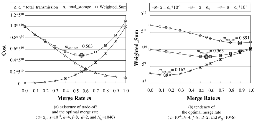
Figure 8: The existence of trade off and the optimal merge rate.

Experiment 1: accuracy as $\alpha$ is varied
Figure 9 shows experimental results as $\alpha$ is varied. We have different optimal merge rates for different scale factors as shown in this figure. From Figure 9, we see that $ratio_{m}$ is 0.905 to 2.619. Other than the value of 2.619 when $\alpha$ is $\alpha_{0}\cdot 10^{-1}$, $ratio_{m}$ is approximately 1.0 for all the other values of $\alpha$. That is, the optimal merge_rate measured from the experimental data is almost the same as that obtained from the analysis. Besides, we see that the value of $ratio_{w}$ is 0.929 to 1.0. That is, the values of Weighted_Sum measured from the experimental data are very close to those obtained from the analysis. As we see from the result of this experiment, as $\alpha$ increases, the weight of the total transmission cost increases relative to the weight of the total storage cost and, thus, the optimal value is determined toward reducing the total transmission cost – toward making the optimal merge_rate close to 1.

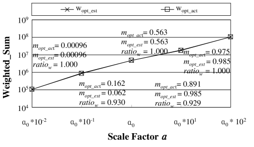
Figure 9: Optimal merge rate as $\alpha$ is varied($s$=$10^{-4}$, $h$=4, $f$=8, $d$=2, and $N_{Q}$=1046).

Experiment 2: accuracy as $c$ is varied
Figure 10 shows the experimental results as the cover is varied. We use different query sets for different covers (we use $N_{Q}$=101 when $c$=0.01, $N_{Q}$=1046 when $c$=0.1, and $N_{Q}$=52685 when $c$=0.99). From Figure 10, we see that $ratio_{m}$ is 0.00092 to 1.008. Other than the value 0.00092 when the cover is 0.99, $ratio_{w}$ is approximately 1.0 for all the other values of the cover. Besides, we see that the value of $ratio_{w}$ is 0.995 to 1.0. That is, the Weighted_Sum measured from the experiments is similar to that obtained from the analysis. As the cover increases, the difference between the maximum and the minimum amounts of data transmission should decrease. Thus, reduction of total data transmission cost have no significant influence on the total cost if the cover increases. Hence, the optimal value is determined toward reducing the total storage cost – toward making the optimal merge rate close to 0.

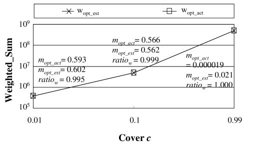
Figure 10: Optimal merge rate as $c$ is varied($\alpha=\alpha_{0}$, $s=10^{-4}$, $h$=4, $f$=8, and $d$=2).

Experiment 3: accuracy as $s$ is varied
Figure 11 shows the experimental results as the selectivity is varied. From Figure 11, we see that $ratio_{m}$ is 0.958 to 1.183 and $ratio_{w}$ is 0.983 to 1.0. The increase of the selectivity is closely related to the increase of the cover. That is, if the selectivity increases while the number of queries is fixed, then the cover of the original queries increases as well, and, thus, like the case of varying the cover, the optimal value moves toward reducing the total storage cost – toward making the optimal merge rate close to 0.

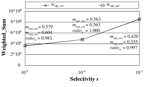
Figure 11: Optimal merge rate as $s$ is varied($\alpha=\alpha_{0}$, $h$=4, $f$=8, $d$=2, and $N_{Q}$=1046).

Experiment 4: accuracy as $h$ is varied
Figure 12 shows the experimental results as the height is varied. We see that $ratio_{m}$ is 0.993 to 1.088 and $ratio_{w}$ is 0.993 to 1.0. When the height of the sensor network increases, the data transmission cost increases faster than the memory usage cost. This stems from the fact that the data sent are accumulated at each tier. Thus, the optimal value moves toward reducing the total data transmission cost – toward making the optimal merge rate close to 1.

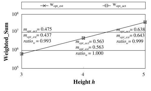
Figure 12: Optimal merge rate as $h$ is varied($\alpha=\alpha_{0}$, $s=10^{-4}$, $f$=8, $d$=2, and $N_{Q}$=1046).

Experiment 5: accuracy as $f$ is varied
Figure 13 shows the experimental results as the fanout is varied. We see that $ratio_{m}$ is 0.993 to 1.088 and $ratio_{w}$ is 0.994 to 1.0.

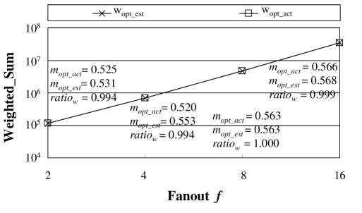
Figure 13: Optimal merge rate as $f$ is varied($\alpha=\alpha_{0}$, $s=10^{-4}$, $h$=4, $d$=2, and $N_{Q}$=1046).

Experiment 6: accuracy as $d$ is varied
Figure 14 shows the experimental results as the dimension is varied. We see that $ratio_{m}$ is 0.993 to 1.088 and $ratio_{w}$ is 0.997 to 1.0.

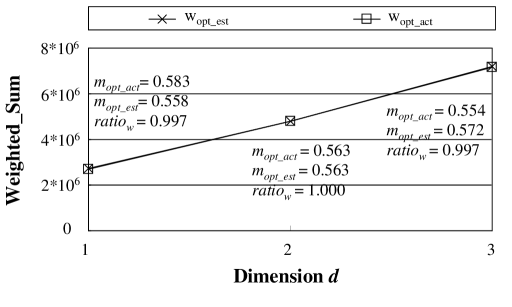
Figure 14: Optimal merge rate as $d$ is varied($\alpha=\alpha_{0}$, $s=10^{-4}$, $h$=4, $f$=8, and $N_{Q}$=1046).

5.2.2 Performance merit of our approach

Experiment 7: performance as $\alpha$ is varied
Figure 15 shows the experimental result as $\alpha$ is varied. Here, we have different merge rates estimated for different scale factors (we use $m_{opt\_est}$=0.00096 when $\alpha$=$\alpha_{0}\cdot 10^{-2}$, $m_{opt\_est}$=0.062 when $\alpha$=$\alpha_{0}\cdot 10^{-1}$, $m_{opt\_est}$=0.563 when $\alpha$=$\alpha_{0}$, $m_{opt\_est}$=0.985 when $\alpha$=$\alpha_{0}\cdot 10^{1}$, and $m_{opt\_est}$=0.985 when $\alpha$=$\alpha_{0}\cdot 10^{2}$)). From this figure, we can see that $gain_{w}$ is 0.989 to 84.995. Except for the value 0.989 when $\alpha$ equals $\alpha_{0}~{}\cdot~{}10$, $gain_{w}$ is 1.004 to 84.995, that is, Weighted_Sum in the progressive approach is smaller than Weighted_Sum in the iterative approach. The exception happens due to the fact that the cover model used in this paper (see Figure 7) is an approximation of the cover in the real environment, and this introduces some error between the actual cost and the estimated cost. From these results, we see that our approach greatly improves the performance over the approach proposed by Xiang et al.[19] when memory usage is the prevailing cost(i.e., $\alpha$ is small), while giving a competitive performance when data transmission is the prevailing cost(i.e., $\alpha$ is large).

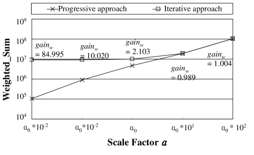
Figure 15: The performance of progressive approach and iterative approach as $\alpha$ is varied($s=10^{-4}$, $h$=4, $f$=8, $d$=2, and $N_{Q}$=1046).

Experiment 8: performance as $c$ is varied
Figure 16 shows the experimental result as the cover is varied. Here, we have different merge rates estimated for different covers (we use $m_{opt\_est}$=0.602 when $c$=0.01, $m_{opt\_est}$=0.562 when $c$=0.1, and $m_{opt\_est}$=0.021 when $c$=0.99). We have different query sets for different covers (we use $N_{Q}$=101 when $c$=0.01, $N_{Q}$=1046 when $c$=0.1, and $N_{Q}$=52685 when $c$=0.99). We see that $gain_{w}$ ranges from 1.019 to 2.498. This result shows that our approach outperforms Xiang et al.’s approach in the entire range of the cover. It also shows that, as the cover increases, the performance benefit of our approach over Xiang et al.’s approach decreases. The benefit of query merge with respect to the storage amount becomes maximum when the cover approaches 1.0. In this case, all the original queries are merged into one query in both our approach and the Xiang et al.’s approach; as a result, the total transmission amounts and the total storage amounts of the two approaches become similar and, therefore, the weighted sums of the two approaches become similar as well. Our proposed approach shows more performance benefit when the cover of the original queries is smaller. The case is more likely to happen in a real environment.

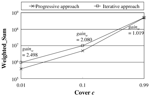
Figure 16: The performance of progressive approach and iterative approach as $c$ is varied($\alpha=\alpha_{0}$, $s=10^{-4}$, $h$=4, $f$=8, and $d$=2).

Experiment 9: performance as $s$ is varied
Figure 17 shows the experimental result as the average selectivity is varied. We have different merge rates estimated for different selectivities (we use $m_{opt\_est}$=0.604 when $s$=$10^{-5}$, $m_{opt\_est}$=0.563 when $s$=$10^{-4}$, and $m_{opt\_est}$=0.355 when $s$=$10^{-3}$). We see that $gain_{w}$ ranges from 1.262 to 2.666. This result shows that our approach outperforms Xiang et al.’s approach in the entire range of selectivity. It also shows that, as the selectivity increases, the performance benefit of our approach decreases. As already mentioned in the experiment that compares the optimal merge rates obtained from the experimental data with those obtained from the analysis, if the selectivity increases, then the cover increases as well causing the decrease of performance benefit as we see in Figure 17. Thus, our proposed approach shows more performance benefit when the selectivity of the original queries is smaller.

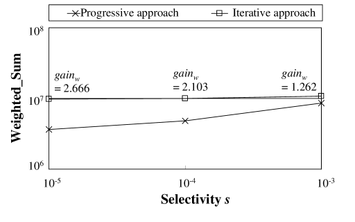
Figure 17: The performance of progressive approach and iterative approach as $s$ is varied($\alpha=\alpha_{0}$, $h$=4, $f$=8, $d$=2, and $N_{Q}$=1046).

Experiment 10: performance as $h$ is varied
Figure 18 shows the experimental result as height of the hierarchical sensor network is varied. We have different merge rates estimated for different heights (we use $m_{opt\_est}$=0.437 when $h$=3, $m_{opt\_est}$=0.563 when $h$=4, and $m_{opt\_est}$=0.643 when $h$=5). We see that $gain_{w}$ ranges from 1.973 to 2.220. This result shows that our approach outperforms Xiang et al.’s approach in the entire range of the height. It also shows that as the height increases, the performance benefit of our approach increases slightly. The reason for this increase is that the total storage amount in the iterative approach increases faster than in the progressive approach as the height increases. That is, in the iterative approach the same set of merged queries are stored in all sensor nodes regardless of the tier whereas, in our progressive approach, a smaller number of queries are stored as the tier goes lower. Thus, our approach shows more performance benefit when the height of the sensor network is larger.

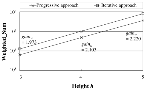
Figure 18: The performance of progressive approach and iterative approach as $h$ is varied($\alpha=\alpha_{0}$, $s=10^{-4}$, $f$=8, $d$=2, and $N_{Q}$=1046).

Experiment 11: performance as $f$ is varied
Figure 19 shows the experimental result as the fanout of the sensor network is varied. We have different merge rates estimated for different fanouts (we use $m_{opt\_est}$=0.531 when $f$=2, $m_{opt\_est}$=0.553 when $f$=4, $m_{opt\_est}$=0.563 when $f$=8, and $m_{opt\_est}$=0.568 when $f$=16). In the result, $gain_{w}$ ranges from 2.103 to 2.159. We observe that for all ranges of $f$, the performance of our approach is better than that of the iterative approach.

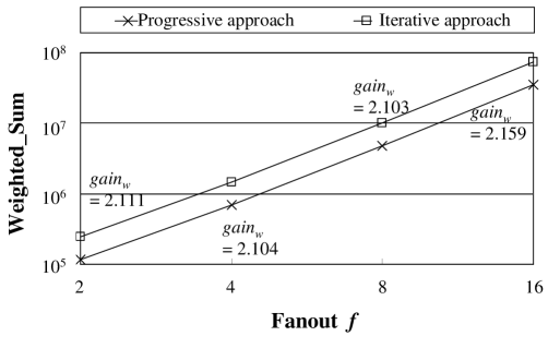
Figure 19: The performance of progressive approach and iterative approach as $f$ is varied($\alpha=\alpha_{0}$, $s=10^{-4}$, $h$=4, $d$=2, and $N_{Q}$=1046).

Experiment 12: performance as $d$ is varied
Figure 20 shows the experimental result as the dimension of a query is varied. We have different merge rates estimated for different dimensions (we use $m_{opt\_est}$=0.558 when $d$=1, $m_{opt\_est}$=0.563 when $d$=2, and $m_{opt\_est}$=0.572 when $d$=3). In the result, $gain_{w}$ ranges from 1.842 to 2.157. We observe that for all ranges of $f$, the performance of our approach is better than that of the iterative approach.

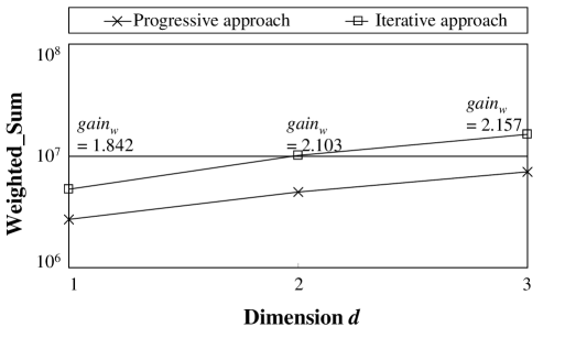
Figure 20: The performance of progressive approach and iterative approach as $d$ is varied($\alpha=\alpha_{0}$, $s=10^{-4}$, $h$=4, $f$=8, and $N_{Q}$=1046).

In summary, the experimental results show that our approach outperforms Xiang et al.’s approach by up to 84.995 times as $\alpha$ is varied except when $\alpha$ is equal to $\alpha_{0}~{}\cdot~{}10$. The results also show that our approach outperforms Xiang et al.’s approach by up to 2.666 times as the following other parameters are varied: the cover, average selectivity, dimension of original queries, and the height, fanout of the hierarchical sensor network.

6 Conclusions

In this paper, we have proposed progressive processing as a new approach to processing continuous range queries in hierarchical sensor networks. The contribution of this paper are summarized as follows.

First, we have proposed a progressive processing model that considers the trade-off between energy and storage. This model takes advantage of the characteristics of the hierarchical sensor networks in which higher capability sensor nodes are deployed at a tier closer to the server. It also has the advantage of reducing the cost of building the network by reducing the storage cost at lower tier nodes, which are larger in number. We also have presented query merging and query processing algorithms for this model.

Second, based on the proposed model, we have proposed a method for optimizing the total cost (formulated as the weighted sum of the energy and storage costs) according to the given weight, and have proposed a method for systematically building a hierarchical sensor network that minimizes the total cost.

Third, we have verified the merit of the proposed approach through extensive experiments. In the experiments for evaluating the accuracy of the proposed cost model, the results show that the ratio of the optimal cost measured over that obtained from the analytical cost model is 0.929 to 1.0. From these results we see that a hierarchical sensor network with near-optimal total cost can be built using the proposed model. In the experiments for evaluating the query processing performance, the results show that our approach outperforms the approach proposed by Xiang et al.[19] by up to 84.995 times. Moreover, if the height of the sensor network increases, our approach shows a better performance than Xiang et al.’s approach. Thus, we can see that our approach is suitable for a large-scale sensor network.

In conclusion, our approach provides a new framework for building a large-scale hierarchical sensor network that efficiently processes a large number of queries while considering the trade-off between the energy consumed and the storage required.

For further work, we plan to improve the query processing model and algorithms to consider different data and query distributions as well as different query types such as aggregate queries.

7 Acknowledgement

This work was supported by the Korea Science and Engineering Foundation (KOSEF) and the Korean Goverment (MEST) through the NRL Program (No. R0A-2007-000-20101-0).

Appendix-A Derivation of Formula for Total_Transmission and Total_Storage

Derivation of total_transmission

The total amount of data sent, denoted as total_transmission, is the sum of the amounts of data sent by all nodes at each tier while they are relayed to the server. Eq.(8) shows the formula for computing total_transmission.

$$total\_transmission = \sum_{i=2}^{h}(Amt\_data_{i}~{}\cdot~{}\sum_{j=2}^{i}(c_{j}))$$

$$\mbox{where}~{}c_{j} = j^{th}$$ the cover of merged queries stored at the  tier, and

$$Amt\_data_{i} = i^{th}$$ the amount of data generated by the sensor nodes at the  tier (8)

In Eq.(8), $c_{j}$ is formulated as follows using the definition of the cover model (see Figure 7) and the merge_rate.

$$c_{j}~{}=~{}\widehat{cover}(N_{Q}~{}\cdot~{}m^{j-1})$$ (9)

where $N_{Q}~{}\cdot~{}m^{i-1}$ is the number of queries stored at the $j^{th}$ tier (note $N_{Q}$ is the number of queries stored in the server (at the $1^{st}$ tier) and $m$ is the merge rate between two nodes in adjacent tiers (see Table 1)). In the same Eq.(8), $Amt\_data_{i}$ is formulated as follows, based on the assumption that each sensor node generates only one data element per unit time.

$$Amt\_data_{i} = (\mbox{the~{}number~{}of~{}sensor~{}nodes~{}at~{}the~{}$i^{th}$~{}tier})~{}\cdot~{}(\mbox{the~{}size~{}of~{}a data~{}element})$$ (10)

$$= f^{i-1}~{}\cdot~{}Size_{de}$$

By substituting $c_{j}$ and $Amt\_data_{i}$ in Eq.(8) with those from Eq.(9) and Eq.(10), we can rewrite the formula for total_transmission as follows.

$$total\_transmission = \sum_{i=2}^{h}(Amt\_data_{i}~{}\cdot~{}\sum_{j=2}^{i}(c_{j}))$$

$$= \sum_{i=2}^{h}(Size_{de}~{}\cdot~{}f^{i-1}~{}\cdot~{}\sum_{j=2}^{i}(c_{j}))$$

$$= \sum_{i=2}^{h}(Size_{de}~{}\cdot~{}f^{i-1}~{}\cdot~{}\sum_{j=2}^{i}(\widehat{cover}(N_{Q}~{}\cdot~{}m^{j-1})))$$

$$= \sum_{i=2}^{h}(Size_{de}~{}\cdot~{}f^{i-1}~{}\cdot~{}\sum_{j=2}^{i}(-a~{}\cdot~{}m^{j-1}~{}\cdot~{}N_{Q}+b))$$

$$\mbox{where}~{}a = \frac{\displaystyle s~{}\cdot~{}(1~{}-~{}c)}{\displaystyle c~{}-~{}s}\,~{}\mbox{and}\,~{}b~{}=~{}1~{}+~{}a$$ (11)

Derivation of total_storage

The total amount of memory used, denoted as total_storage, is the sum of the amounts of memory used by all nodes at all tiers. Eq.(12) shows the formula for computing total_storage.

$$total\_storage = \sum_{i=2}^{h}(Amt\_mem_{i})$$

$$\mbox{where}~{}Amt\_mem_{i} =$$ the amount of memory needed to store (12)

the merged queries in all sensor nodes at the $$i^{th}$$ tier

The number of merged queries stored in a sensor node at the $i^{th}$ tier is formulated as $N_{Q}~{}\cdot~{}m^{i-1}$ using Eq.(12) and Eq.(9). Thus, $Amt\_mem_{i}$ is formulated as in Eq.(13).

$$Amt\_mem_{i} = (\mbox{the~{}number~{}of~{}merged~{}queries~{}stored~{}in~{}all~{}sensor~{}nodes~{}at~{}the ~{}$i^{th}$~{}tier})$$ (13)

$$\cdot (\mbox{the amount~{}of~{}memory~{}needed~{}for~{}storing~{}one~{}query})$$

$$= f^{i-1}~{}\cdot~{}N_{Q}~{}\cdot~{}m^{i-1}~{}\cdot~{}2\cdot Size_{de}$$

By substituting $Amt\_mem_{i}$ from Eq.(13) into Eq.(12), the formula for total_storage can be rewritten as follows.

$$total\_storage = \sum_{i=2}^{h}(Amt\_mem_{i})$$ (14)

$$= \sum_{i=2}^{h}(f^{i-1}~{}\cdot~{}N_{Q}~{}\cdot~{}m^{i-1}~{}\cdot~{}2~{}\cdot~{}Size_{de})$$

$$= \sum_{i=2}^{h}(~{}2~{}\cdot~{}Size_{de}~{}\cdot~{}f^{i-1}~{}\cdot~{}N_{Q}~{}\cdot~{}m^{i-1})$$

References

- [1] Abiteboul, S. et al., “The Lowell Database Research Self-Assessment.,” Communications of the ACM(CACM), Vol. 48, No. 5, pp. 111- 118, May 2005.
- [2] Akyildiz, I. F., Melodia, T., Chowdhury, K. R., “A Survey on Wireless Multimedia Sensor Networks,” Computer Networks, Vol. 51, No. 4, pp.921-960, March 2007.
-
[3]
EarthNet News (available at
http://earth.esa.int/object/index.cfm?fobjectid=5106). - [4] Ganu, S., Zhao, S., Raju, L., Anepu, B., Seskar, I., and Raychaudhuri, D., Architecture and Prototyping of an 802.11-Based Self-Organizing Hierarchical Adhoc Wireless Network (SOHAN), White Paper, Rutgers University, March 2004.
- [5] Gui, C. and Mohapatra, P., “Power Conservation and Quality of Surveilance in Target Tracking Sensor Networks,” In Proc. 10th Annual Int’l Conf. on Mobile Computing and Networking(MOBICOM), Philadelphia, PA, pp. 129-143, September 2004.
- [6] Li, X., Kim, Y.-J., Govindan, R., and Hong, W., “Multi-Dimensional Range Queries in Sensor Networks,” In Proc. 1st Int’l Conf. on Embedded Networked Sensor Systems (ACM Sensys), Los Angeles, California, pp. 63-75, November 2003.
- [7] Lim, H., Lee, J., Lee, M., Whang, K., and Song, I., “Continuous Query Processing in Data Streams Using Duality of Data and Queries,” In Proc. 2006 ACM SIGMOD Int’l Conf. on Management of Data, pp. 313-324, Chicago, Illinois, June 26-29, 2006.
- [8] Madden, S. R., Franklin, M. J., Hellerstein, J. M., and Hong, W., “TinyDB: An Acqusitional Query Processing System for Sensor Networks,” ACM Transactions on Database Systems (TODS), Vol. 30, No. 1, pp. 122-173, March 2005.
- [9] Maple Software (available at http://www.maplesoft.com).
- [10] Muller, R. and Alonso, G., “Efficient Sharing of Sensor Networks,” In Proc. 3rd IEEE Int’l Conf. on Mobile Ad-hoc and Sensor Systems(MASS), Vancouver, Canada, pp.109-118, October 2006.
- [11] NOVAC project (available at http://www.novac-project.eu).
-
[12]
Palo, C., “Towards Next Generation Wireless Sensor Networks –
Rethinking Middleware Design,” November 2007 (available at
research.microsoft.com/en-us/um/people/costa
/getslides.aspx?doc=midsens07.pdf ). - [13] Park, S. M., “Technical Trend of Sensor Network Node Platform & OS,” Electronics and Telecommunications Trends, ETRI, Vol. 21, No. 1, pp. 14-24, February 2006.
- [14] Qingguang, Z., Yanling, C., and Juan,.L., “A Lightweight Key Management Protocol for Hierarchical Sensor Networks”, In Proc. 7th Int’l Conf. on Parallel and Distributed Computing, Applications and Technologies (PDCAT), Taipei, Taiwan, pp. 379-382, December 2006.
- [15] Ratnasamy, S., Karp, B., Shenker, S., Estrin, D., Govindan, R., Yin, L., and Yu, F., “Data-Centric Storage in Sensornets with GHT, a Geographical Hash Table,” Mobile Networks and Applications, Vol. 8, No.4, pp. 427-442, August 2003.
- [16] Singh, M. and Prasanna, V. K., “A Hierarchical Model for Distributed Collaborative Computation in Wireless Sensor Networks ,” In Proc. the 17th Int’l Symposium on Parallel and Distributed Processing(IPDPS), Nice, France, pp. 166-258, April 2003.
- [17] Srivastava, U., Munagala, K., and Windom, J., “Operator Placement for In-Network Stream Query Processing,” In Proc. the 24th ACM SIGACT-SIGMOD-SIGART Symposium on Principle of Database Systems(PODS), Baltimore, Maryland, USA, pp. 250-258, June 2005.
- [18] Trigoni, N., Yao, Y., Demers, A. J., Gehrke, J., and Rajaraman, R., “Multi-query optimization for Sensor Networks,” In Proc. 1st Int’l Conf. on Distributed Computing in Sensor Systems(DCOSS), Marina del Rey, CA, pp. 307-321, July 2005.
- [19] Xiang, S., Lim, H. B., and Tan, K.-L., “Impact of Multi-Query Optimization in Sensor Networks,” In Proc. Workshop on Data Management in Sensor Networks(DMSN’06), Seoul, Korea, pp. 7-12, September 2006.
- [20] Xiang, S., Lim, H. B., and Tan, K.-L., “Multiple Query Optimization for Wireless Sensor Networks,” In Proc. International Conference on Data Engineering(ICDE’07), Istanbul, Turkey, pp. 1339-1341, April 2007.
- [21] Yao, Y. and Gehrke, J.,“The Cougar Approach to In-Network Query Processing in Sensor Networks,” SIGMOD Record, Vol. 31, No. 1, pp.9-18, March 2002.
- [22] Yu, W., Le, T. N., Xuan, D., and Zhao, W.,“Query Aggregation for Providing Efficient Data Services in Sensor Networks,” In Proc. 1st IEEE Int’l Conf. on Mobile Ad-hoc and Sensor Systems(MASS), Florida, pp.31-40, October 2004.