Tomography of correlation functions for ultracold atoms via time-of-flight images

Abstract

We propose to utilize density distributions from a series of time-of-flight images of an expanding cloud to reconstruct single-particle correlation functions of trapped ultra-cold atoms. In particular, we show how this technique can be used to detect off-diagonal correlations of atoms in a quasi-one-dimensional trap, where both real- and momentum- space correlations are extracted at a quantitative level. The feasibility of this method is analyzed with specific examples, taking into account finite temporal and spatial resolutions in experiments.

I Introduction

Ultracold atomic gas provides a controllable platform to study strongly correlated many-body physics, which has attracted strong interest recently review . To reveal many-body properties of the underlying systems, normally one needs to detect some kinds of correlation functions. The detection method for atomic systems is typically very different from detection of condensed matter materials. For solid state systems, linear responses provide a useful method to measure the system correlation functions. For ultracold atomic gases, measuring linear response is possible but not always convenient. A powerful and widely used detection method for atomic gases is based on the time-of-flight (TOF) imaging technique review , which is unique to these atomic systems and has no counterpart in condensed matter materials. During the TOF imaging, one measures the light absorption of an expanding atomic cloud released from the external trap. The light absorption gives information of the density distribution of the expanded cloud, which, under some approximation, is proportional to the initial momentum distribution of the atomic gas prior to expansion. Therefore, the TOF imaging provides us a useful technique to extract the diagonal single-particle correlation function in the momentum space. With only the diagonal correlation in the momentum space, in general it is inadequate to reconstruct the real space correlation function. To fulfill this gap, several methods have been proposed to introduce additional control techniques, and measure the real space correlation functions based on the atomic interference dettmer-01 or the Fourier sampling duan . Some of the real-space correlations can also be inferred from measurement of the two-particle correlations which can be extracted from noise spectroscopy noise .

In this manuscript, we discuss a method to extract information about full single-particle correlations in both the momentum and the real spaces, by measuring the density profiles in the TOF images at different expansion times. Our detection proposal is in the spirit of tomography in the spatial-temporal space, where the full correlations are reconstructed through certain algorithms. The method is strict for (quasi) one-dimensional (1D) systems, and can be applied to higher-dimensional cases where the symmetry is applied to reduce the effective dimensionality. Compared with other detection schemes, this method is more direct in the sense that it relies solely on the TOF images and does not require introduction of other challenging control techniques. Besides, it only utilizes the mean density distribution of the resulting images, for which the detection is in general significantly easier than the measurement of quantum noise of the corresponding images. As an example of applications of this detection method, we consider a quasi-1D Bose gas and demonstrate that all off-diagonal single-particle correlations can be reconstructed from a series of TOF images at various expansion times. The feasibility of this method is analyzed under realistic experimental conditions of spatial and temporal resolutions.

The remainder of this manuscript is organized as follows. In Section II, we discuss the main reconstruction formalism by analyzing the ballistic expansion process of an atomic gas and showing how the single-particle correlations are obtained from density profiles in the TOF images. We consider both the quasi-1D case and the high-dimensional cases where one can either separate variables or have spherical symmetry to reduce dimensionality. As a by-product, we also derive in this section the formula for the far-field limit, where the initial momentum distribution is directly connected with the final density profile, and obtain the quantitative conditions under which this far-field-limit formula is valid. After introducing the general formalism, to illustrate its applications we give an example in Section III by considering a quasi-1D Bose gas, and demonstrate how correlations are reconstructed from the TOF images. Finally, we discuss the effects from finite spatial and temporal resolutions and conclude that this method is applicable within present experimental conditions.

II Formalism for reconstruction of correlation functions

In most experiments, the atomic gas is usually prepared inside some external optical or magnetic trap. When the system achieves its thermal equilibrium, one detects the properties of its underlying many-body state through the TOF imaging. To perform this TOF imaging measurement, one turns off the external trap such that the atomic gas starts to expand in space. For simplicity, we assume a ballistic expansion process where the atomic interaction is negligible during the expansion. This is typically a good approximation for optical lattice experiments when the atomic density is not high note1 . For strongly interacting atoms near a Feshbach resonance, to get the ballistic expansion, one needs to first sweep the magnetic field to the deep BEC or BCS side to turn off the interaction, as done in many experiments.

For a ballistic expansion, the atomic cloud freely expands and the expansion dynamics is already known. Before turn-off of the trap, the system is in thermal equilibrium, and its single-particle correlation function is denoted by $\mathcal{G}_{0}(\mathbf{r},\mathbf{r}^{\prime})=\langle\phi_{0}^{\dagger}(\mathbf{r})\phi_{0}(\mathbf{r}^{\prime})\rangle$, where $\phi_{0}(\mathbf{r})\equiv\phi(\mathbf{r,}t\leq 0)$ is the atomic field operator, which is either bosonic or fermionic corresponding to bosons or fermions, respectively. Assume at time $t=0$ the trap is turned off, and we measure the density profile $\langle n(\mathbf{r},t)\rangle\equiv\langle\phi^{\dagger}(\mathbf{r,}t)\phi(\mathbf{r},t)\rangle$ of the atomic cloud at various expansion time $t$. From the measured density $\langle n(\mathbf{r},t)\rangle$ note2 , we would like to reconstruct the full single-particle correlation $\mathcal{G}_{0}(\mathbf{r},\mathbf{r}^{\prime})$. Note that this reconstruction is in general impossible for a three-dimensional system, where $\mathcal{G}_{0}(\mathbf{r},\mathbf{r}^{\prime})$ depends on six variables and $\langle n(\mathbf{r},t)\rangle$ has only four variables. The correlation $\mathcal{G}_{0}(\mathbf{r},\mathbf{r}^{\prime})$ therefore contains more information than the density profile $\langle n(\mathbf{r},t)\rangle$. However, we will show in the following that for any quasi-1D systems, the reconstruction of the correlation functions can be done exactly. Furthermore, the correlation can also be obtained for many practical high-dimensional systems, where the system either possesses spherical symmetry or can be separated in variables for the single-particle correlations.

The expansion dynamics of the atomic cloud is well described by the Schrodinger equation for the atomic field operator (taking $\hslash=1$):

$$i\partial_{t}\phi(\mathbf{r},t)=-\frac{\nabla^{2}}{2m}\phi(\mathbf{r},t).$$ (1)

The solution of this equation in the momentum space is simply given by

$$\phi(\mathbf{k},t)=\mathcal{U}_{0}(t)\phi_{0}(\mathbf{k})=\phi_{0}(\mathbf{k})e^{-ik^{2}t/2m},$$ (2)

where $\phi(\mathbf{k},t)$ is the Fourier transform of the field operator $\phi(\mathbf{r},t)$ at time $t$, $\mathcal{U}_{0}$ is the free propagator, $m$ is the atomic mass, and initial conditions are $\phi(\mathbf{k},t=0)=\phi_{0}(\mathbf{k})$. The expectation value of density distribution thus takes the form

$$\langle n(\mathbf{r},t)\rangle = \frac{1}{\left(2\pi\right)^{6}}\iint d\mathbf{k}_{1}d\mathbf{k}_{2}e^{-i(\mathbf{k}_{1}-\mathbf{k}_{2})\cdot\mathbf{r}}$$ (3)

$$\times e^{i(\mathbf{k}_{1}^{2}-\mathbf{k}_{2}^{2})t/2m}\langle\phi_{0}^{\dagger}(\mathbf{k}_{1})\phi_{0}(\mathbf{k}_{2})\rangle.$$

It is useful to define new variables $\mathbf{k}_{+}\equiv\mathbf{k}_{1}+\mathbf{k}_{2}$ and $\mathbf{k}_{-}\equiv\mathbf{k}_{1}-\mathbf{k}_{2}$, with which the density expectation value becomes

$$\langle n(\mathbf{r},t)\rangle = \frac{1}{2\left(2\pi\right)^{6}}\iint d\mathbf{k}_{+}d\mathbf{k}_{-}e^{-i\mathbf{k}_{-}\cdot\left(\mathbf{r}/\tilde{t}-\mathbf{k}_{+}\right){\tilde{t}}}$$ (4)

$$\times\left\langle\phi_{0}^{\dagger}\left(\frac{\mathbf{k}_{+}+\mathbf{k}_{-}}{2}\right)\phi_{0}\left(\frac{\mathbf{k}_{+}-\mathbf{k}_{-}}{2}\right)\right\rangle,$$

where ${\tilde{t}}\equiv t/2m$ is defined to simplify the notation.

An important feature of the density profile in Eq. (4) is that for long evolution time $\tilde{t}$ (called the far-field-limit), the exponential term gives a rapid-oscillating phase factor except for the region around the point $(\mathbf{k}_{-}=0,\mathbf{k}_{+}=\mathbf{r}/{\tilde{t}})$. As a consequence, the integration over $\mathbf{k}_{+}$ and $\mathbf{k}_{-}$ is dominated by the contribution from such region, leading to an approximating form for the density expectation value (see the derivation in Appendix A)

$$\langle n(\mathbf{r},t)\rangle\approx\frac{1}{2\left(2\pi\right)^{3}{\tilde{t}}}\left\langle\phi_{0}^{\dagger}\left(\frac{\mathbf{r}}{2\tilde{t}}\right)\phi_{0}\left(\frac{\mathbf{r}}{2\tilde{t}}\right)\right\rangle.$$ (5)

Notice that the final density profile is directly proportional to the initial momentum distribution via a scaling relation $\mathbf{k}=\mathbf{r}/(2\tilde{t})$. This formula has been widely used for interpretation to the measurement result from the TOF images. For this far-field-limit to be valid, the expansion time needs to be sufficiently long. Quantitatively, it has to satisfy the following condition

$$\left(\Delta\mathbf{k}_{+}\cdot\Delta\mathbf{k}_{-}\right)\tilde{t}\gg 1.$$ (6)

Here, $\Delta\mathbf{k}_{+}$ and $\Delta\mathbf{k}_{-}$ are characteristic scales for the extension (variation) of single-particle correlation function $\mathcal{G}_{0}(\mathbf{k}_{1},\mathbf{k}_{2})$ along the $\mathbf{k}_{+}$ and $\mathbf{k}_{-}$ directions, respectively. The derivation of this condition for the far-field limit is shown in Appendix A.

The extraction of momentum distribution only utilizes the measured density profile in the far-field limit. The density distribution measured at other expansion times contain more information about the single-particle correlations. Next, we discuss how to inverse the relation in Eq. (3), and to reconstruct the off-diagonal correlations from TOF images. We first discuss in detail the 1D system where the reconstruction algorithm is exact, and then generalize the method to higher dimensional cases by reducing to a set of 1D problems when symmetry or separability arguments are applicable.

Let us consider a quasi-1D atomic cloud along the $x$-direction where the transverse degrees of freedom are frozen through a deep potential such as an optical lattice. The density profile $\left\langle n(x,t)\right\rangle$ thus depends on correlation functions through a double-integration with two phase factors along the spatial and temporal directions, respectively. One can think about performing a double Fourier transform to inverse the relation. Specifically, we obtain

$$\langle{\tilde{n}}(p,\omega)\rangle \equiv \int_{-\infty}^{\infty}dx\int_{0}^{\infty}dt\langle n(x,t)\rangle e^{-i\left(px+\omega t\right)}$$ (7)

$$=\frac{m}{2|p|}\left\langle\phi_{0}^{\dagger}\left(\frac{-2m\omega/p-p}{2}\right)\phi_{0}\left(\frac{-2m\omega/p+p}{2}\right)\right\rangle$$

$$-\frac{i}{4\pi}\frac{2m}{p}\mathcal{PV}\left(\int dk_{+}\frac{\left\langle\phi_{0}^{\dagger}\left(\frac{k_{+}-p}{2}\right)\phi_{0}\left(\frac{k_{+}+p}{2}\right)\right\rangle}{-2m\omega/p+k_{+}}\right)$$

for the cases with $p\neq 0$, which is connected with the off-diagonal momentum correlations and hence of particular interest.

Notice that the integration over time is for $t>0$ only, since all the density profiles are obtained after turn-off of the trap. This partial Fourier transform hence generates the principal value ($\mathcal{PV}$) integral on the right hand side of Eq. (7). This expression can be significantly simplified if the single-particle correlations are real. This condition is equivalent to assume a time-reversal symmetry throughout the system. In fact, for systems in a stationary frame, it is very unlikely for the time-reversal symmetry to be broken as long as there is no such symmetry breaking term in the Hamiltonian note3 . Under this condition, the principal value integral is purely imaginary, and the off-diagonal momentum correlation (with $k_{-}\neq 0$) can be solved as

$$\left\langle\phi_{0}^{\dagger}(k_{1})\phi_{0}(k_{2})\right\rangle$$ (8)

$$= 4|k_{-}|\mathrm{Re}\left[\int_{0}^{\infty}d{\tilde{t}}\int_{-\infty}^{\infty}dxe^{-ik_{-}(k_{+}{\tilde{t}}-x)}\left\langle n(x,t)\right\rangle\right].$$

Therefore, with the measured density profile $\left\langle n(x,t)\right\rangle$ at different time $t$, we can reconstruct all the momentum correlations through the formulae (5) and (8). With the knowledge of all momentum space correlations, the real space correlation function can also be obtained via a double Fourier transform. After substituting the expression (8), the integration over two momentum indices can be carried out analytically, leading to

$$\left\langle\phi_{0}^{\dagger}(x_{1})\phi_{0}(x_{2})\right\rangle$$ (9)

$$= \frac{1}{2\pi}\mathrm{Re}\left[\int_{0}^{\infty}d{\tilde{t}}\int_{-\infty}^{\infty}dx\left|\frac{x_{-}}{{\tilde{t}}^{2}}\right|e^{-ix_{-}\left(2x-x_{+}\right)/4{\tilde{t}}}\left\langle n(x,t)\right\rangle\right].$$

Here, the variables $x_{+}\equiv x_{1}+x_{2}$ and $x_{-}\equiv x_{1}-x_{2}$ are defined to simplify notations. The convergence of the integration over time for $t\rightarrow 0$ is usually guaranteed by cancelation from the fast oscillation in the exponent $e^{-ix_{-}\left(2x-x_{+}\right)/4{\tilde{t}}}$. These two simple relations between the measured density profiles and the initial correlation functions in both the momentum space [Eq. (8)] and the real space [Eq. (9)] are the central results for this section.

After introducing the reconstruction scheme for the 1D case, next we consider the problem in higher dimensions. Since the density profile $\left\langle n(\mathbf{r},t)\right\rangle$ is in fact a function of $d$(spatial)$+1$(temporal) variables, in the most general case it is no longer possible to fully reproduce the single-particle correlation, which is a function of $d\times d$ variables. However, if the system has some properties which allows us to reduce dimensionality, a similar procedure can still be performed on the reduced problems. For instance, if there exists spherical symmetry in 3D systems, the field operator can be written as $\phi(\mathbf{r},t)=\phi(r,t)$, where $r$ is the radial distance. In this case, the free expansion process is governed by the Schrodinger equation in spherical coordinate,

$$i\partial_{t}\phi(r,t)=-\frac{1}{2m}\left(\partial_{r}^{2}+\frac{2}{r}\partial_{r}\right)\phi(r,t).$$ (10)

By defining a new operator $\psi(r,t)=r\phi(r,t)$, the equation above becomes

$$i\partial_{t}\psi(r,t)=-\frac{\partial_{r}^{2}}{2m}\psi(r,t).$$ (11)

Notice that this equation has exactly the same structure as the Schrodinger equation (1) for the 1D case, which allows us to obtain the single particle correlation function $\langle\phi_{0}^{\dagger}(r)\phi_{0}(r^{\prime})\rangle=\langle\psi_{0}^{\dagger}(r)\psi_{0}(r^{\prime})\rangle/(rr^{\prime})$ from the density distribution $n(r,t)$ via a similar procedure as Eq. (9).

The reconstruction scheme can also be generalized to higher dimensional cases when the correlation functions are separable, i.e.,

$$\left\langle\phi^{\dagger}(\mathbf{r},t)\phi(\mathbf{r}^{\prime},t)\right\rangle=\prod_{i=x,y,z}\left\langle\phi_{i}^{\dagger}(r_{i},t)\phi_{i}(r_{i}^{\prime},t)\right\rangle.$$ (12)

In this case, the higher dimensional problem can be effectively reduced to a set of 1D problems and then treated separately using the same method discussed above.

III Correlations in one-dimensional quasi-condensates: an example

In the previous section, we have shown how to reconstruct the single-particle correlations from the measured density profile for 1D systems and higher-dimensional cases where symmetry or separability can be used to reduce the effective dimensionality. To illustrate applications of this general formalism, in this section we consider a specific example and show hot to reconstruct the correlation functions for bosonic atoms in a quasi-1D trap. The reconstruction formula in Eqs. (8) and (9) are given as double integrals of the measured density profiles. In realistic experiments, however, one can take only a finite number of images, and each image contains a finite number of resolvable data points. In the following discussion, we will take into account the finite spatial and temporal resolutions, and show that a good approximation to the correlation function can be inferred already from about a dozen of images.

In this example, we consider a quasi-1D Bose gas trapped through either a highly elongated cigar-shaped potential gorlitz-01 or a deep transverse two-dimensional optical lattice kinoshita-04 . In this quasi-1D geometry with strong radial confinement $\omega_{\rho}$, atoms at low temperatures are essentially frozen at the ground state of the radial harmonic trap. Thus the radial wave function is governed by

$$\phi_{\rho}(y,z)=\sqrt{\frac{1}{\pi a_{\rho}^{2}}}e^{-(y^{2}+z^{2})/(2a_{\rho}^{2})},$$ (13)

where $a_{\rho}\equiv 1/\sqrt{m\omega_{\rho}}$ characterizes the extension of the radial wave function and $m$ is the atomic mass. When $a_{\rho}$ is much greater than the effective length scale of interatomic potential $R_{e}$, the gas can be described with an effective 1D interaction rate 1Dgas

$$g_{\mathrm{1D}}=\frac{2a_{s}}{ma_{\rho}^{2}},$$ (14)

where $a_{s}$ denotes the $s$-wave atomic scattering length in free space.

The static single-particle correlation function in this quasi-1D system has been calculated by evaluating phase fluctuation effects around the saddle point condensate densities. This process gives the axial real-space correlation function 1Dgas

$$\mathcal{G}_{0}(x,x^{\prime})\approx\sqrt{n_{0}(x)n_{0}(x^{\prime})}e^{-1/2F_{s}(x,x\prime)},$$ (15)

where $n_{0}(x)$ is the zero-temperature Thomas-Fermi density distribution in the axial direction

$$n_{0}(x)=\frac{1}{g_{\mathrm{1D}}}\left(\mu_{0}-\frac{m\omega_{x}^{2}x^{2}}{2}\right)\theta\left(\mu_{0}-\frac{m\omega_{x}^{2}x^{2}}{2}\right),$$ (16)

and the function $F_{s}(x,x^{\prime})$ takes the form

$$F_{s}(x,x^{\prime})=\frac{4T\mu_{0}}{3N\omega_{x}^{2}}\left|\ln\frac{(1-x/R_{\mathrm{TF}})(1+x^{\prime}/R_{\mathrm{TF}})}{(1+x/R_{\mathrm{TF}})(1-x^{\prime}/R_{\mathrm{TF}})}\right|.$$ (17)

Here, $T$ is the temperature, $N$ is the total atom number, $\mu_{0}$ denotes the chemical potential at the trap center, and $R_{\mathrm{TF}}=\sqrt{2\mu_{0}/(m\omega_{x}^{2})}$ is the Thomas-Fermi cloud radius along the axial direction (with a small axial trapping frequency $\omega_{x}$). We emphasize that we only use the correlation function in Eq. (15) as an example to illustrate our detection method. The derivation of this correlation is irrelevant for our following purpose.

We assume a ballistic expansion of the atomic gas along the axial direction for TOF imaging (the transverse trap is still on), which allows us to numerically simulate the expansion process with the initial correlation given by Eq. (15), and obtain the expected density distribution at each measurement time. Using these resulting density profiles, then we try to reconstruct the corresponding correlation functions using Eqs. (5) and (8). From the derivation in the last section, if we have infinite spatial resolution and take an infinite number of images, we should be able to obtain exactly the same correlation function as shown in Eq. (15). So the purpose here is actually to analyze the effects from finite spatial and temporal resolutions as is the case for realistic experiments. In the following discussion, we assume to take only $10\sim 30$ images, and for each image we only know $\left\langle n(x,t)\right\rangle$ for a discrete set of points from the finite spatial resolution. In Fig. 1, we show a typical set of results for $\left\langle n(x,t)\right\rangle$ at various times. Notice that we assume here a finite spatial resolution of $\Delta x=20\mu$m with $R_{\mathrm{TF}}/\Delta x\approx 8$, which gives about $16$ readable data points from the absorption image at the very beginning of $t=0$.

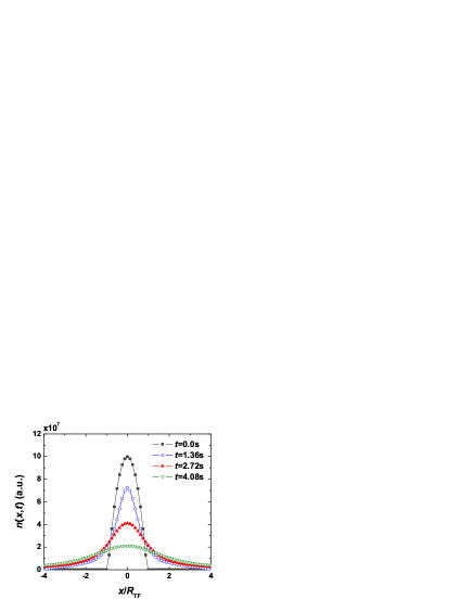
Figure 1: (Color online) The density profiles along the axial direction at different expansion times for a quasi-1D Bose gas released from the trap. Throughout the paper, we consider a gas of ⁸⁷Rb atoms with total number $N=10^{4}$ interacts via s-wave scattering length $a_{s}=5.45$ nm. The gas is confined in a cigar-shaped potential with the trapping frequencies $\omega_{x}=2\pi\times 30$ Hz and $\omega_{\rho}=2\pi\times 20000$ Hz. The Thomas-Fermi radius along the axial direction is $R_{\mathrm{TF}}\approx 160\mu$m. Such a system can be realized in a 2D optical lattice with the lattice constant $d=426$ nm and the lattice depth $V_{0}=10E_{\mathrm{R}}$, where $E_{\mathrm{R}}$ is the recoil energy. In this plot, we consider a spatial resolution of $\Delta x=20\mu$m, which gives about $16$ data points (squares) from the absorption image at the very beginning of $t=0$. The temperature of the system is assumed to be $T=20\omega_{x}$.

First, let us try to extract the correlation function in momentum space using the formula in Eq. (8). In Fig. 2, we plot the reconstructed off-diagonal correlation $\langle\phi_{0}^{\dagger}(k)\phi_{0}(-k)\rangle$ using the simulated density profiles. There are three important features one can read from this plot. First, the reconstructed correlations are fairly close to the expected exact values obtained from the Fourier transform of the real-space correlation in Eq. (15), especially when the correlation is sizable such that the error is relatively small. Second, the reconstruction fails for $k$ very close to zero. This is because the TOF images taken here are not for an infinite time duration. For the reconstruction, we take the data points within the ranges given by $x_{\mathrm{max}}$ and $t_{\mathrm{max}}$ for coordinates and time, respectively. Since the reconstruction relies on a Fourier transform, these finite ranges set a limit for the resolution in the momentum space. In fact, by increasing the evolving time $t_{\mathrm{max}}$, which simultaneously requires an increase of $x_{\mathrm{max}}$ since the cloud expands more, we can push the reconstruction further towards $k=0$. Third, except for the region $k\sim 0$, the results are insensitive to the time split between two subsequent images. Notice that since we use $M_{t}=30$ images for both reconstructions in Fig. 2, the trial with longer evolving time has larger time split. The result, however, is fairly close to the other trial for $k$ not very close to $0$.

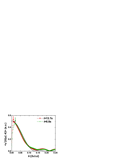
Figure 2: (Color online) The momentum-space correlation $\langle\phi_{0}^{\dagger}(k)\phi_{0}(-k)\rangle$ reconstructed from the density profiles via Eq. (8), where a total of $M_{t}=30$ images are taken equidistantly between $t=0$ and the maximal expansion time $t_{\mathrm{max}}=6.8$ s (triangles) and $t_{\mathrm{max}}=13.7$ s (dots). The results are compared with the expected exact values from a direct Fourier transform of Eq. (15) (solid line). The oscillatory behavior for large $k$ is an artificial effect due to the sudden drop of the Thomas-Fermi density distribution at the cloud edge. Notice that the reconstruction fails for $k\rightarrow 0$ (hollow points), while the questionable region shrinks (arrows) with increasing $t_{\mathrm{max}}$ and $x_{\mathrm{max}}$. In this plot, we assume a spatial resolution of $\Delta x=40\mu$m with $R_{\mathrm{TF}}/\Delta x=4$, which gives about $8$ data points from the absorption image at the very beginning of $t=0$. Other parameters used here are the same as the ones in Fig. 1.

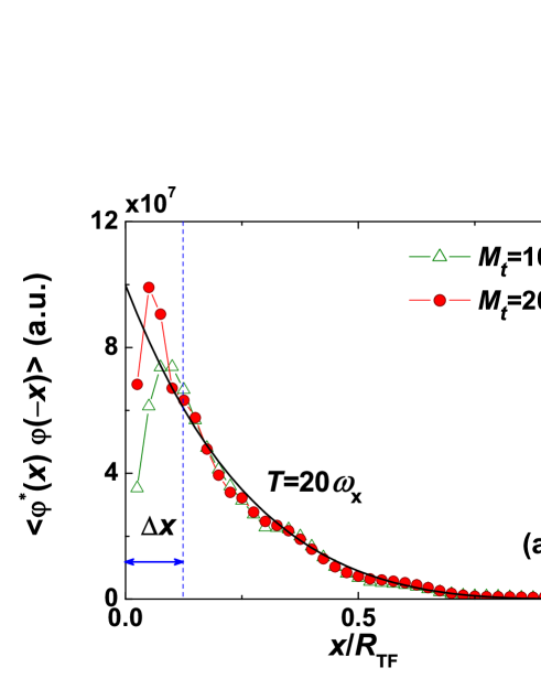
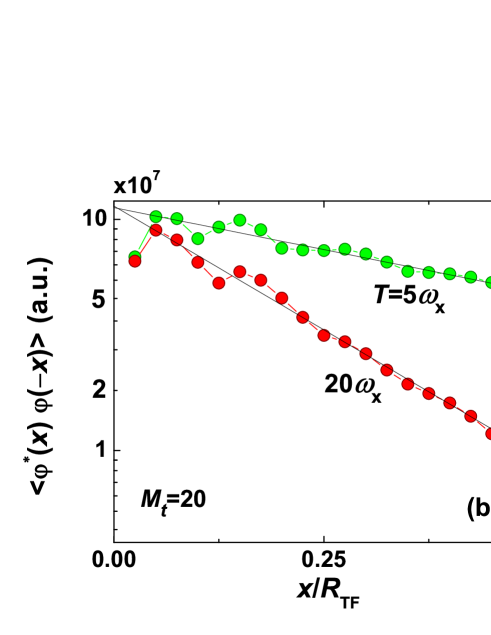
Figure 3: (Color online) (a) The real-space correlation $\langle\phi_{0}^{\dagger}(x)\phi_{0}(-x)\rangle$ reconstructed from the density profiles via Eq. (9), where the maximal expansion time $t_{\mathrm{max}}=6.8$ s are sliced equidistantly to obtain $M_{t}=10$ (triangles) and $M_{t}=20$ (dots) images. Results are compared with the expected values of Eq. (15) (solid line). (b) Log plot of $\langle\phi_{0}^{\dagger}(x)\phi_{0}(-x)\rangle$ around the center of the cloud at different temperatures. Exponential decay can be clearly observed in this plot, with the correlation length given by an exponential fit (solid lines). Other parameters used here are the same as the ones in Fig. 2.

Next, we analyze the correlation function in the real space. In Fig. 3(a), we show the reconstructed correlations of $\langle\phi_{0}^{\dagger}(x)\phi_{0}(-x)\rangle$ from the density profiles via Eq. (9). The most striking feature of this plot is that the spatial correlations can be obtained very precisely for $x$ not too close to $0$, using as few as $M_{t}=10$ images. Even in the questionable region for $x$ less than the spatial resolution $\Delta x$, some information can still be extracted by applying linear interpolation between image pixels, and the precision in that region can be significantly enhanced when more images are used for reconstruction. In Fig. 3(b), the real-space correlations for two different temperatures are plotted in log scale, showing explicitly the exponential decay around the center of the trap with corresponding correlation lengths.

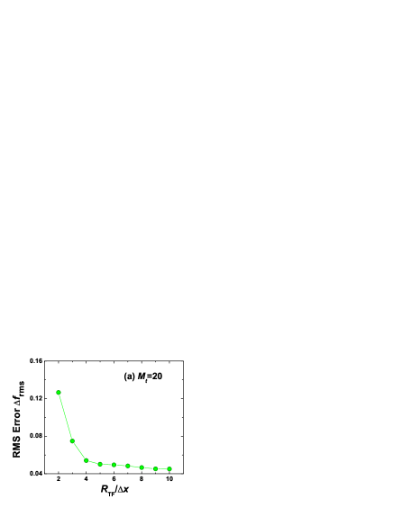
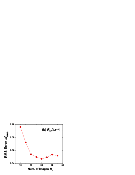
Figure 4: (Color online) Normalized RMS error of the reconstructed correlations for $\mathcal{G}_{0}(x,-x)$, (a) as a function of the spatial resolution $\Delta x$ with a fixed number of images $M_{t}=20$, and (b) as a function of the number of images $M_{t}$ with a fixed spatial resolution $R_{\mathrm{TF}}/\Delta x=4$. The system is at temperature $T=20\omega_{x}$, with total expansion time $t_{\mathrm{max}}=6.8$ s. Other parameters are the same as the ones in Fig. 1.

Finally, we investigate how the increase of spatial and temporal resolutions can enhance the reconstruction precision. To quantitatively evaluate the precision, we consider the real-space correlation as illustrated in Fig. 3(a), and define the root-mean-square (RMS) of the error

$$\Delta f_{\mathrm{rms}}=\frac{1}{n_{0}(0)}\sqrt{\frac{\sum_{i=1}^{N_{x}}[\mathcal{G}_{0}(x_{i},-x_{i})-\mathcal{G}_{0}^{\mathrm{TOF}}(x_{i},-x_{i})]^{2}}{N_{x}}},$$ (18)

where $\mathcal{G}_{0}^{\mathrm{TOF}}(x_{i},-x_{i})$ is the reconstructed correlation from the TOF images, and the function is normalized to the center density $n_{0}(0)$. Notice that this normalized RMS error will depend on the number of reconstruction sampling points $N_{x}$, which is $40$ as in Fig. 3(a). But its value will not change much with different $N_{x}$ and will follow the same trend with variation of the resolutions. In Fig. 4, we show the normalized RMS error in Eq. (18) as functions of spatial [Fig. 4(a)] and temporal [Fig. 4(b)] resolutions, respectively. Notice that the error decreases rapidly by increasing resolutions in both variables, as one would expect. Besides, the value of the error saturates to a fairly small number $(\sim 5\%)$ around $R_{\mathrm{TF}}/\Delta x\sim 4$ and $M_{t}\sim 20$, respectively, indicating that the technique is quite feasible under the present technology.

IV Conclusion

In summary, we have proposed a method to reconstruct the full static single-particle correlation functions in both the momentum and the real spaces for cold atomic gas by measuring the density profiles at different expansion times with the time-of-flight imaging. The method applies to quasi-1D systems and can be generalized to higher dimensions when symmetry or separability arguments can be used to reduce the effective dimensionality. As an example, we consider a quasi-1D Bose gas and demonstrate how real- and momentum-space correlations are reconstructed at a quantitative level. The feasibility of this method is analyzed by evaluating the reconstruction error with various spatial and temporal resolutions, and the result suggests that the correlations can be inferred with pretty good precision already with a dozen of images at practical spatial resolution.

Appendix A Far-field Limit

For simplicity of the notation, here we derive the far-field limit formula only for the 1D case. The extension of the formula to higher dimensions is straightforward. In the 1D case, the expectation value of the density distribution in Eq. (4) takes the following form

$$I=\frac{1}{2\left(2\pi\right)^{2}}\int dx\int dye^{ixyt}f(x,y),$$ (19)

where $f(x,y)$ represents the single-particle correlation function. The correlation function $f(x,y)$ spreads over certain ranges, with the characteristic length scales along the $x$ and $y$ directions denoted by $\Delta X$ and $\Delta Y$, respectively. The integration over $dy$ in Eq. (19) can be performed after a Fourier transform, leading to

$$I = \frac{1}{4\pi}\int dx\mathscr{F}(x,s=xt)$$ (20)

$$= \frac{1}{4\pi t}\int ds\mathscr{F}(s/t,s),$$

where $\mathscr{F}(x,s)$ is the Fourier transform of $f(x,y)$ as a function of $y$. Notice that from the Fourier transformation theorem, the function $\mathscr{F}$ must spread along the $x$ and $s$ directions with the characteristic length scales given by $\Delta X$ and $1/\Delta Y$, respectively.

In the expression above, the integration over $s$ is essentially along the line $(s/t,s)$. For large enough time $t$, this line is almost the $s$-axis. Thus, the result can be approximated by

$$I\approx\frac{1}{4\pi t}\int ds\mathscr{F}(0,s)=\frac{1}{4\pi t}f(0,0),$$ (21)

where the second step is given by Fourier transforming the $\mathscr{F}$ function back to the $(x,y)$ plane. The last equation gives the far-field limit result.

In order to make this approximation valid, the function $\mathscr{F}(s/t,s)$ and $\mathscr{F}(0,s)$ should be close to each other for typical values of $s$. As the function $\mathscr{F}(s/t,s)$ has characteristic length scales $\Delta X$ and $1/\Delta Y$ respectively along the $x$ and $s$ directions, the condition $s/t\ll\Delta X$ must be fulfilled for $s$ within the typical range given by $1/\Delta Y$. Therefore, we conclude that the far-field limit given by Eq. (21) is valid when the following condition is satisfied

$$\Delta X\Delta Yt\gg 1.$$ (22)

The above argument can be easily generalized to higher dimensional cases, leading to the far-field limit condition as shown in Eq. (6).

References

- (1) For a review, see I. Bloch and M. Greiner, Adv. At. Mol. Opt. Phys. 53, 1 (2005); W. Ketterle, D.S. Durfee, and D.M. Stamper-Kurn, in Bose-Einstein condensation in atomic gases, edited by M. Inguscio, S. Stringari, and C.E. Wieman, IOS Press, Amsterdam (1999).
- (2) S. Dettmer et al. Phys. Rev. Lett. 87, 160406 (2001).
- (3) L.-M. Duan, Phys. Rev. Lett. 96, 103201 (2006).
- (4) E. Altman, E. Demler, M.D. Lukin, Phys. Rev. A 70, 013603 (2004); S. Folling et al., Nature 434, 481 (2005); M. Greiner et al., Phys. Rev. Lett. 94, 110401 (2005); M. Schellekens et al., Science 310, 638 (2005); Z. Hadzibabic et al., Nature 441, 1118 (2006).
- (5) For a Bose system with Bose-Einstein condensation, the interatomic interaction can have non-trivial effect on the time-of-flight images and cause a broadening of the condensate peak. In such a case, since the condensate and thermal parts can be separated in the images through a bimodal fit, this interaction effect can be addressed by numerically evolving the time-dependent Gross-Pitaevskii equation for the condensate, while leaving the momentum correlation of the thermal part almost unchanged (see, e.g., G.-D. Lin, W. Zhang, and L.-M. Duan, Phys. Rev. A, 77, 043626 (2008), for details).
- (6) What one measures in experiments is the atomic density integrated along the imaging direction. However, for the quasi-1D case or the 3D case with spherical symmetry as discussed in this paper, one can reconstruct the density profile from its column integration (see Y. Shih et al., Phys. Rev. Lett. 97, 030401 (2006)).
- (7) For 2D Bose gases, time-reversal symmetry can be spontaneously broken by creating vortex-antivortex pairs below the BKT transition temperature. However, since the excitation energy increases logarithmically with the vortex pair size, for temperature not too close to the transition temperature, vortex pairs are tightly combined and we can resume a time-reversal symmetry for the coarse-grained wave function.
- (8) A. Gölitz et al., Phys. Rev. Lett. 87, 130402 (2001).
- (9) T. Kinoshita, T. Wenger, D.S. Weiss, Science 305, 1125 (2004).
- (10) D.S. Petrov, G.V. Shlyapnikov, and J.T.M. Walraven, Phys. Rev. Lett. 85, 3745 (2000); D.L. Luxat and A. Griffin, Phys. Rev. A 67, 043604 (2003); S. Richard et al., Phys. Rev. Lett. 91, 010405 (2003).