Triggered Star Formation in a Double Shell near W51A

Abstract

We present Heinrich Hertz Telescope CO observations of the shell structure near the active star-forming complex W51A to investigate the process of star formation triggered by the expansion of an H II region. The CO observations confirm that dense molecular material has been collected along the shell detected in Spitzer IRAC images. The CO distribution shows that the shell is blown out toward a lower density region to the northwest. Total hydrogen column density around the shell is high enough to form new stars. We find two CO condensations with the same central velocity of 59 km s^-1 to the east and north along the edge of the IRAC shell. We identify two YSOs in early evolutionary stages (Stage 0/I) within the densest molecular condensation. From the CO kinematics, we find that the H II region is currently expanding with a velocity of 3.4 km s^-1, implying that the shell’s expansion age is $\sim$ 1 Myr. This timescale is in good agreement with numerical simulations of the expansion of the H II region (Hosokawa & Inutsuka). We conclude that the star formation on the border of the shell is triggered by the expansion of the H II region.

1. Introduction

Feedback from massive stars has significant impact on the surrounding interstellar medium (ISM), and may even trigger star formation in the vicinity of their expanding H II regions (Elmegreen & Lada, 1977). An expanding H II region sweeps up an ambient interstellar medium and accumulates the material between the ionization front and the shock front. The material collected on the border of the H II region will form a shell structure and would appear as a ring on the plane of the sky. Second-generation stars may form when the compressed layer becomes gravitationally unstable or the expanding shell provides enough external pressure to initiate collapse of a pre-existing molecular clump. There are relatively few good examples of this process published to date (e.g., Deharveng et al., 2003; Zavagno et al., 2006; Watson et al., 2008; Pomarès et al., 2009). Therefore, identifying other cases of shell structures around OB stars, together with detailed study of the associated interstellar matter, will provide valuable understanding of the triggered star formation process.

High spatial resolution of the Spitzer Space Telescope makes it possible to routinely detect these shell structures at mid-infrared wavelengths. Churchwell et al. (2006) found 322 shell structures from the Galactic Legacy Infrared Mid-Plane Survey Extraordinaire (GLIMPSE; Benjamin et al., 2003). They reported that many of the infrared shells coincide with known H II regions produced by O and early-B type stars. About 7% of the shells in their catalog reveal a multiple morphology. The shell structure we present in this paper is a multiple bubble consisting of N102 and N103 in their catalog.

In this paper, we use infrared and CO observations to study the double-shell structures and their interactions with the surrounding ISM. Infrared observations from Spitzer show the morphology of the shell and reveal the YSOs possibly formed by triggering in the surrounding ISM. Direct observation of molecular gas around the shell is necessary (1) to confirm that ambient molecular material is indeed associated with the expanding H II region, (2) to find any clumpy material that could condense to form new stars, and (3) to learn the physical properties (e.g., density of accumulated molecules) of the ambient ISM into which the shell is expanding. These observations will enable us to determine whether or not it is possible to form stars by the triggering effect of the H II region.

This paper is organized as follows. We introduce our CO observations and the data sets used in this paper in § 2. In § 3.1, we describe the morphology of the N102 and N103 region. We identify the ionizing star in § 3.2 and any young stellar objects (YSOs) around the shell in § 3.3. In § 4 we present the distribution and kinematics (§ 4.1) and physical conditions (§ 4.2) of the molecular cloud associated with the shell. We discuss the triggered star formation on the border of the H II region in § 5. We summarize our results in § 6.

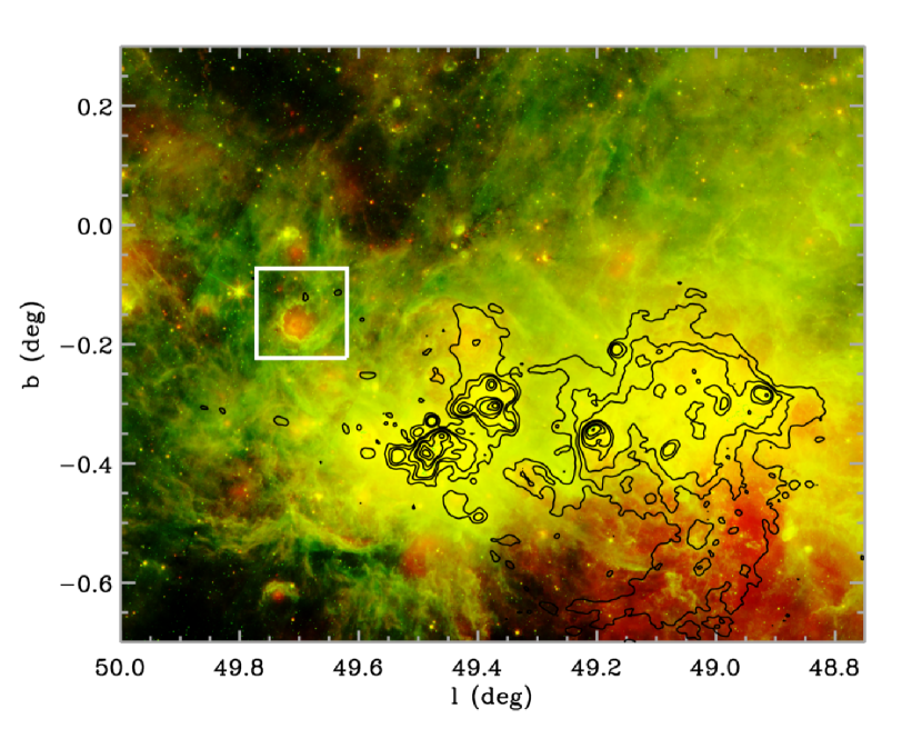
Figure 1.— A color image of the W51 complex composed of MIPS 24 $\micron$ (red) and IRAC 8.0 $\micron$ (green). The contour map shows 21 cm radio continuum emission. It was made by combining VLA data and Effelsberg 100-m telescope data (Koo & Moon, 1997). The contour levels are $-$0.015, 0.015, 0.05, 0.10, 0.3, 0.5, 1.0, 1.5, and 2.4 Jy beam^-1. The white box shows the outline of the shell area (Figure 2).

2. Observations and Data Analysis

We have carried out ¹²CO and ¹³CO (J=2-1) line observations of the W51 H II region complex with the 10 meter Heinrich Hertz Telescope (HHT) on Mt. Graham, Arizona. The whole map covers a 1.25$\arcdeg$ $\times$ 1.00$\arcdeg$ region centered at ($l,b$) = ($49.375\arcdeg$, $-0.2\arcdeg$). In this paper, we extract a 0.152$\arcdeg$ $\times$ 0.150$\arcdeg$ region centered at ($l,b$) =(49.696°, $-$0.148°) which includes the shell structure. The ¹²CO and ¹³CO (J=2-1) line observations were mapped with on-the-fly (OTF) scanning in longitude at 10$\arcsec$ per second with row spacing of 10$\arcsec$ in latitude. We used the 1.3mm ALMA band 6 dual polarization sideband-separating receiver with a 4-6 GHz IF band. The receiver was tuned with the ¹²CO (J=2-1) line at 230.538 GHz in the upper sideband and ¹³CO (J=2-1) line at 220.399 GHz in the lower sideband. The spectrometers, one for each of the two polarizations and the two sidebands, were filter banks with 256 channels of 1 MHz width and separation. Beam efficiency was 0.85, which we adopt for all the data.

Data for each CO isotopomer were processed with the CLASS reduction package (from the University of Grenoble Astrophysics Group), by removing a linear baseline and convolving the data to a square grid with 10$\arcsec$ grid spacing. The intensity scales for the two polarizations were determined from observations of W51D made just before the OTF maps. System temperatures were calibrated by the standard ambient temperature load method (Kutner & Ulich, 1981) after every other row of the map grid. Further analysis was done with the Miriad software package (Sault et al., 1995). Although the data observed early in the program with a different receiver were noisier than with the ALMA receiver, data quality was improved after combining all of the data using ($1/T_{sys}$)² weighting. To further reduce the noise of the images without significantly sacrificing angular resolution, we convolved the maps with a 16$\arcsec$ (FWHM) Gaussian. This increases the effective resolution from 32$\arcsec$ to 36$\arcsec$, but smooths over the 10$\arcsec$ OTF raster pattern, improving the final image quality. The two polarizations were averaged for each sideband, yielding images with rms noise per pixel and per velocity channel of 0.16 and 0.07 K-T${}_{A}^{*}$ for the ¹²CO and ¹³CO transition respectively. The average rms noise level of the ¹²CO map is larger than ¹³CO because several sub-fields of ¹²CO map were observed just one time with the noisier receiver.

¹³CO (J=1-0) data covering the same region as our mapping area were extracted from the Galactic Ring Survey (GRS) with spectral resolution of 0.2 km s^-1, angular resolution of 46$\arcsec$ and sampling of 22$\arcsec$. The rms noise level of the GRS data when smoothed to 1.3 km s^-1 velocity resolution is 0.08 K-T${}_{A}^{*}$. The intensities on an antenna temperature scale were divided by the main beam efficiency of 0.48 to convert to main-beam brightness temperature.

The Galactic Legacy Infrared Midplane Survey Extradodinaire (GLIMPSE) I survey observed the Galactic plane ($65\arcdeg<|l|<10\arcdeg$ for $|b|<1\arcdeg$) with the four mid-IR bands (3.6, 4.5, 5.8, and 8.0 $\micron$) of the Infrared Array Camera (IRAC; Fazio et al., 2004) on the Spitzer Space Telescope. The Midinfrared Imaging Photometer for Spitzer Galactic plane Survey (MIPSCAL; Carey et al., 2005) is a legacy program covering the inner Galactic plane, $65\arcdeg<|l|<10\arcdeg$ for $|b|<1\arcdeg$, at 24 and 70 µm with the Multiband Imaging Photometer for Spitzer (MIPS; Rieke et al., 2004) on the Spitzer Space Telescope. We analyzed mosaicked images of four IRAC bands and MIPS 24 $\micron$. The resolutions of IRAC and MIPS 24 $\micron$ are 1$\farcs$2 and 2$\farcs$4, respectively.

We use the GLIMPSE I Catalog which consists of point sources that are detected at least twice in one band with a S/N $>$ 5. The GLIMPSE I Catalog also includes $JHK_{s}$ flux densities from the 2MASS point source catalog (Skrutskie et al., 2006). MIPS 24 $\micron$ fluxes were obtained from running the GLIMPSE pipeline on the MIPSGAL BCD mosaics (Meade, private communication). We extract 24 $\micron$ point-sources with $S/N>7$, then bandmerge the 24 $\micron$ sources with the GLIMPSE Catalog sources using a 2$\farcs$0 correlation radius. The final source list consists of all 8 bands combined: 2MASS $JHK_{s}$, IRAC (3.6, 4.5, 5.8, and 8.0µm), and MIPS 24 $\micron$.

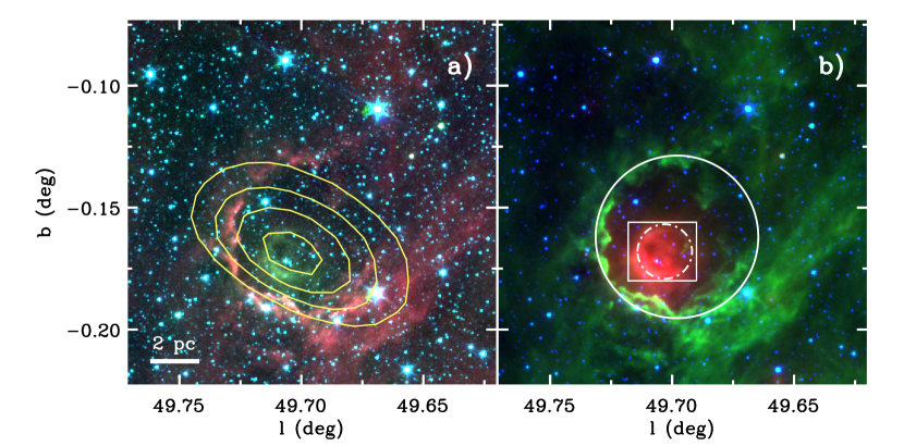
Figure 2.— (a) Composite image of IRAC 8.0 $\micron$ (red), IRAC 4.5 $\micron$ (green), and IRAC 3.6 $\micron$ (blue). Contours show Westerbork Synthesis Radio Telescope(WSRT) 327 MHz radio continuum (Taylor et al., 1996). Contour levels are 0.07, 0.12, 0.16, and 0.21 Jy beam^-1. Scale bar on the left bottom represents a size at the distance of 5.7 kpc. (b) Composite image of MIPS 24 $\micron$ (red), IRAC 8.0 $\micron$ (green), and IRAC 4.5 $\micron$ (blue). Outer solid circle represents a shell size of 2$\arcmin$ radius centered on ($l,b$) = (49.698$\arcdeg$, -0.162$\arcdeg$) of N102. Inner dash-dotted circle represents N103 with 0.67$\arcmin$ radius centered on ($l,b$) = (49.703$\arcdeg$, -0.168$\arcdeg$) (Churchwell et al., 2006). The white box is the outline enlarged in Figure 3.

3. Properties of the Region

3.1. Spitzer Images and Radio Continuum

Figure 1 shows a two-color composite image of Spitzer IRAC 8 $\micron$ (green) and MIPS 24 $\micron$ (red) data from the GLIMPSE and MIPSGAL Legacy data bases, for a 1°$\times$ 1.25 °area including the W51 star-forming region. The contours outline the radio continuum emission from the ionized gas and supernova remnant (Koo & Moon, 1997). The double shell structure studied in this paper is located in the white boxed area of Figure 1.

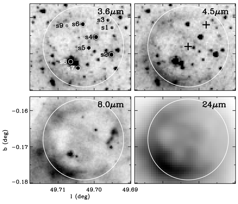
Figure 3.— Images of the central region at the indicated wavelengths. Candidate ionizing stars are labeled from s1 to s9 on the 3.6 $\micron$ image. The large circles are centered on N103 and have a radius of 0.67$\arcmin$. Two crosses in 4.5 $\micron$ image are the center of N102 and N103.

Figure 2 shows an enlarged view of this double shell structure from the composite image of IRAC and MIPS bands. The inside and outside shells are N103 and N102, respectively (Churchwell et al., 2006). A bright 8 $\micron$ shell (solid line in Figure 2$b$) encloses bright 24 $\micron$ emission from the inner shell region. IRAC 8 $\micron$ mainly shows the emission of polycyclic aromatic hydrocarbons (PAHs), which are excited in the photodissociation region (PDR). Therefore PAHs emission trace the ionization fronts well. MIPS 24 $\micron$ present the emission of the small dust grains, which is inside of the shell. We note that these shell structures are not visible in any of the 2MASS near-IR images, despite their prominence in the GLIMPSE IRAC data. Average radii of N102 and N103 are 2$\farcm$0 and 0$\farcm$67, corresponding to 3.3 pc and 1.1 pc, respectively. Here we adopt a kinematic distance to the shells as 5.7 kpc, which were deduced from the velocity of the associated molecular material, $V_{LSR}=$ 59 km s^-1 from our HHT observations, and the Galactic rotation curve of Brand & Blitz (1993).

This shell structure lies in the direction of the major star-forming regions in the Galaxy (Avedisova, 2002). This apparent association on the plane of the sky does not prove that the shell results from the expansion of an H II region caused by star formation activity, rather than some other process (e.g., supernova remnant, planetary nebula, etc.). To determine whether our double shell represent is H II region or not, we compile the radio continuum observations at various frequencies: $S_{\rm 4.875\,GHz}$ = 0.55 Jy and $S_{\rm 14.8\,GHz}$ = 0.21 Jy (Wink et al., 1982), $S_{\rm 1.4\,GHz}$ = 0.62 Jy (Condon et al., 1998), $S_{\rm 4.85\,GHz}$ = 0.33 Jy (Gregory et al., 1996), $S_{\rm 327\,MHz}$ = 0.80 Jy (Taylor et al., 1996), $S_{\rm 4.875\,GHz}$ = 0.55 Jy (Altenhoff et al., 1979).

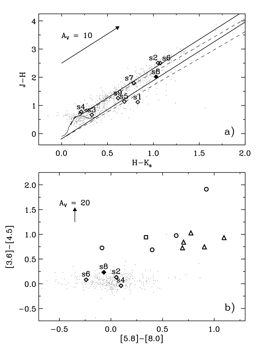
Figure 4.— (a) JHKs color-color plot. The solid and dashed curves represent the locus of main-sequence and giant stars (Bessell & Brett, 1988). The parallel solid and dashed lines, for O6-8V (Koornneef, 1983) and M0V (Bessell & Brett, 1988), are reddening vectors with color excess ratios of 2.07 (Kim et al., 2007) and 1.9 (Okumura et al., 2000), respectively. Reddening vector shows A_V=10 mag. (b) IRAC $[3.6]-[4.5]$ vs. $[5.8]-[8.0]$ color-color plot. Gray dots are all sources detected at each band through the line of sight in the shell region. Open diamonds are stars within the radius of N103 seen in Figure 3. Filled diamond represents a candidate ionizing star. YSO candidates are marked as circles for Stage 0/I, triangles for Stage II, and squares for ambiguous sources. Reddening vector for A_V=20 mag based on the extinction laws of Indebetouw et al. (2005) is shown as a filled arrow.

Table 1Model parameters for YSO candidates

Number	Name	$(\chi^{2})$	$L_{tot}$	$\Delta L_{tot}$	$M_{\star}$	$\Delta M_{\star}$	$\dot{M}_{env}$	$\Delta\dot{M}_{env}$	$A_{V}$	$\Delta A_{V}$	Stage
	(G$l+b$)		($L_{\odot}$)	($L_{\odot}$)	($M_{\odot}$)	($M_{\odot}$)	($M_{\odot}yr^{-1}$)	($M_{\odot}yr^{-1}$)	(mag)	(mag)
1	G49.6510-0.1541	0.01	92	99	3.1	1.0	4.29$\times 10^{-6}$	2.97$\times 10^{-5}$	18.8	9.1	II
2	G49.6548-0.1291	1.30	7408	2937	10.3	1.3	1.30$\times 10^{-6}$	4.83$\times 10^{-5}$	47.5	3.1	II
3	G49.6554-0.1452	0.00	35	37	3.1	0.8	2.86$\times 10^{-6}$	1.27$\times 10^{-5}$	1.4	1.8	II
4	G49.6608-0.1253	2.10	321	625	2.4	2.4	5.17$\times 10^{-5}$	1.39$\times 10^{-4}$	30.6	21.3	0/I
5	G49.6608-0.1458	0.39	2143	3248	8.0	3.8	9.58$\times 10^{-4}$	1.28$\times 10^{-3}$	6.4	7.1	0/I
6	G49.6657-0.1941	0.11	140	236	3.6	1.1	7.74$\times 10^{-6}$	2.85$\times 10^{-5}$	10.7	4.6	Amb
7	G49.6698-0.2161	0.26	26	24	2.2	1.2	1.36$\times 10^{-5}$	2.74$\times 10^{-5}$	4.4	2.3	0/I
8	G49.6713-0.1205	0.17	38	31	3.3	0.4	1.03$\times 10^{-7}$	2.91$\times 10^{-7}$	0.6	0.8	II
9	G49.6776-0.1099	2.59	114	52	3.4	0.4	4.45$\times 10^{-8}$	1.83$\times 10^{-6}$	10.1	2.7	II
10	G49.7256-0.0873	15.05	262	97	4.2	0.3	1.58$\times 10^{-8}$	4.94$\times 10^{-9}$	3.0	1.0	II
11	G49.7261-0.0777	0.98	71	59	3.1	0.8	1.01$\times 10^{-6}$	7.95$\times 10^{-6}$	22.7	9.0	II
12	G49.7309-0.2173	0.35	28	47	1.9	1.1	7.29$\times 10^{-6}$	1.98$\times 10^{-5}$	1.9	1.5	Amb
13	G49.7343-0.1109	0.07	1218	2673	6.2	3.2	2.53$\times 10^{-4}$	5.70$\times 10^{-4}$	11.6	10.3	0/I
14	G49.7355-0.1695	1.62	337	151	5.9	0.9	8.28$\times 10^{-5}$	1.53$\times 10^{-4}$	19.1	7.3	0/I
15	G49.7409-0.1125	0.01	316	136	4.4	0.6	3.41$\times 10^{-7}$	1.12$\times 10^{-5}$	15.4	2.8	II
16	G49.7421-0.1766	4.52	52	64	2.6	1.2	1.59$\times 10^{-5}$	3.77$\times 10^{-5}$	6.9	3.1	Amb
17	G49.7470-0.2130	0.71	52	49	3.0	1.0	2.09$\times 10^{-5}$	5.31$\times 10^{-5}$	4.9	1.9	Amb
18	G49.7552-0.0775	2.94	95	51	3.6	0.8	6.72$\times 10^{-5}$	8.50$\times 10^{-5}$	16.8	10.4	Amb
19	G49.7637-0.0742	0.00	83	176	3.1	0.9	5.06$\times 10^{-6}$	1.60$\times 10^{-4}$	14.3	9.2	II

Taylor et al. (1996) concluded that most sources detected by the Westerbork Synthesis Radio Telescope (WSRT) at 327 MHz and in the IRAS Point Source Catalog are thermal radio sources associated with compact H II regions. Their W1921+1442 is coincident with the shell structure as seen in Figure 2 (a). IRAS fluxes of the source are 1.0, 24.9, 225.8, and 292.5 Jy at 12, 25, 60, and 100 $\micron$. Taylor et al. (1996) selected a ratio of $S_{\rm 60\,\mu m}$ to $S_{\rm 327\,MHz}$ = 200 as the boundary separating thermal and non-thermal radio sources. The ratio of $S_{\rm 60\,\mu m}$ to $S_{\rm 327\,MHz}$ of W1921+1442 is greater than 200, consistent with thermal emission. The IRAS flux ratio also lies in the region $0.5<\log(S_{60}/S_{25})<1.7$ and $0.5<\log(S_{25}/S_{12})<1.4$ occupied by compact H II regions.

We use equation (1) of Simpson & Rubin (1990) to estimate from the radio-continuum flux the number of ionizing Lyman continuum photons $N_{\rm LyC}$ emitted by the exciting star. We assume a fraction of helium recombination photons to excited states $f_{i}=0.65$, an electron temperature $T_{e}=10000$ K and a distance $D=5.7$ kpc. The integrated flux density at 4.85 GHz is 0.33 Jy (Gregory et al., 1996), indicating an ionizing flux of log($N_{\rm LyC})\sim 47.96$ photons per second. This corresponds to a star of spectral type O9V (Martins et al., 2005). The value $S_{\rm 4.875\,GHz}$ = 0.55 Jy (Altenhoff et al., 1979; Wink et al., 1982) gives log($N_{\rm LyC})\sim 48.18$ photons per second, which implies on O8.5V spectral type. The ionizing flux may be a lower limit if there is significant dust absorption in the ionized gas.

3.2. Identifying Ionizing Star

Given that the N102 and N103 structures are shells swept up by expanding H II regions, we try to identify the ionizing stars using NIR photometry. N102 (outer shell) shows a nearly complete circular shape except for the missing region to the north-west which suggests an eruption of the bubble. Ionizing star(s) might be located near the center of the shell where the inner shell (N103) is located. Therefore, we consider stars detected at all 2MASS bands within the inner shell as possible candidates for ionizing star(s). Figure 3 shows the candidate ionizing stars, labeled from s1 to s9, at different IRAC and MIPS bands.

The most likely candidate to be the ionizing source was selected as follows: Using photometry data from the 2MASS and Spitzer catalogs, we placed sources in Figure 3 on color-color diagrams (see Figure 4). Extinction is clearly severe toward the Sagittarius spiral arm tangency at $45\arcdeg<l<51\arcdeg$ including W51, since there is no detectable increase in the star count (Benjamin et al., 2005; Churchwell et al., 2009). Okumura et al. (2000) and Kim et al. (2007) estimated a color excess ratio $E_{J-H}/E_{H-K_{s}}$ of 1.9 and 2.07 toward W51A and W51B, respectively. In the $J-H$ vs. $H-K_{s}$ color-color diagram, we assumed a color excess ratio of 2.07. Although the color excess ratio is measured from the W51B region, the value 2.07 traces the sources in the shell region better than 1.9 measured in W51A (see Figure 4$a$). This excess ratio is at the upper range of $1.73\pm 0.40$ found in the Galactic reddening law study of Indebetouw et al. (2005). Following the criterion by Kim et al. (2007), we rejected sources with $J-K_{s}<2.2$ as foreground sources. Notice how this includes source s4, which despite being located near the center of the N102 structure, presents negligible extinction and has a color consistent with the locus of giant stars by Bessell & Brett (1988); moreover, the source is easily detectable in optical plates from the Digitized Sky Survey (DSS), which would exclude it from being a deeply embedded source. Foreground sources s1 and s3 are also marginally detected in the DSS optical band. Sources s2, s6 and s7, have $J-K_{s}>2.2$ showing significant reddening, but they are located in the region of the diagram corresponding to the extension of the cool Giant locus towards highly reddened values, and thus we also discard them as candidate ionizing sources. The remaining source, s8, is located in a region of the diagram likely to be occupied by deeply embedded O type stars.

Candidate ionizing stars detected in all IRAC bands are located in the group of main-sequence and giant stars around (0,0) in the Spitzer $[3.6]-[4.5]$ vs. $[5.8]-[8.0]$ color-color diagram in Figure 4 (b), indicating that they are not YSOs.

3.3. YSO Candidates

In order to determine whether the expanding H II region is able to trigger the star formation, we investigate if there are newly formed stars in the vicinity of the shell structure. To find YSO candidates associated with the shell structure we use the 2MASS and GLIMPSE point source catalogs. There are 2189 sources in $0.152\arcdeg\times 0.150\arcdeg$ region around N102. We identity a total of 19 YSOs near the shells using the SED fitter of Robitaille et al. (2007) following the procedures described in Povich et al. (2009). The SED fitter includes a grid of 200,000 YSO model spectral energy distributions (SEDs) and finds a model fit using a $\chi^{2}$-minimization. For SED fitting, we use the sources detected in at least four bands ($N_{data}\geq 4$) of the 8 IR bands, consisting of the 4 IRAC bands and the 3 2MASS bands for sources with firm 2MASS identifications in the GLIMPSE Point Source Catalog, and the MIPS 24 $\micron$ flux from the MIPSGAL survey if detected (see Section 2). First, to remove stellar sources, we fit stellar photosphere SEDs to all the sources with $N_{data}\geq 4$. Sources with $\chi^{2}/N_{data}\leq 4$, indicating a good stellar fit, are removed. Because the fitting tool take into accounts extinction (Indebetouw et al., 2005), even highly reddened stars should be removed by this step. Asymptotic giant branch (AGB) stars are removed by fitting AGB star SED templates included in the SED fitting tool.

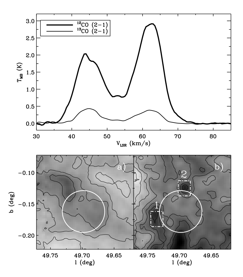
Figure 5.— Top: Average ¹²CO and ¹³CO (J=2-1) spectra seen in Figure 2. Bottom (a) The ¹²CO (J=2-1) intensity integrated between 40 and 50 km s^-1. (b) The ¹³CO (J=2-1) intensity integrated between 56 and 67 km s^-1. The gray scale is from 0 to 44 K km s^-1. Contour levels are 5, 10, 15, 20, 25, 30, and 35 K km s^-1. Circles show the shell size of N102. The dash-dotted rectangles labeled 1 and 2 show the fields of clumps 1 and 2 in Figure 6.

Next, we fit the sources which are poorly fit by stellar photospheres to the YSO models of Robitaille et al. (2006). We allow the distance range to be from 5 to 9 kpc and the interstellar extinction from 0 to 60 mag in V band for fitting YSOs. In the same manner as fitting stellar photospheres, we consider sources with $\chi^{2}/N_{data}\leq 4$ to be good fits. We discard sources not detected at 24 $\micron$ which show 8 $\micron$ flux excesses above an extrapolation of the 3 shorter wavelength IRAC bands. These sources are usually contaminated at 8 $\micron$ by a noise peak or a diffuse background feature.

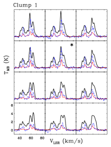
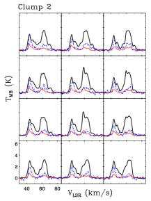
Figure 6.— ¹²CO (J=2-1) (thick solid line), ¹³CO (J=2-1) (thin solid line) and ¹³CO (J=1-0) (dash-dotted line) spectra of clumps 1(left) and 2 (right) seen in the dash-dotted boxes in Figure 5. The spectra have 22$\arcsec$ spacing.

Each YSO stage is defined by a disk mass $M_{\rm disk}$ and an envelope accretion rate $\dot{M}_{\rm env}$ provided by the SED fitting algorithm: Sources are classified as Stage 0/I with $\dot{M}_{\rm env}/M_{\star}>10^{-6}~{}{\rm yr}^{-1}$, Stage II YSOs with $\dot{M}_{\rm env}/M_{\star}<10^{-6}~{}{\rm yr}^{-1}$ and $M_{\rm disk}/M_{\star}>10^{-6}$, and Stage III with $\dot{M}_{\rm env}/M_{\star}<10^{-6}~{}{\rm yr}^{-1}$ and $M_{\rm disk}/M_{\star}<10^{-6}$ (Robitaille et al., 2006). We determine the evolutionary stage of each source using the relative probability distribution for the Stages of all the good-fit models. Note that we use the term “Stage” to distinguish the evolutionary state of the theoretical model from the term “Class” which derives from the observed SED (Evans et al., 2009). The good-fit models of each source are defined by

$$\chi^{2}-\chi^{2}_{\rm min}\leq 2N_{\rm data},$$ (1)

where $\chi^{2}_{\rm min}$ is the goodness-of-fit parameter for the best-fit model. The relative probability of each good-fit model is estimated according to

$$P(\chi^{2})=e^{-(\chi^{2}-\chi^{2}_{\rm min})/2}$$ (2)

and is normalized. After a probability distribution for the evolutionary Stage of each source is constructed from the Stages of all the good-fit models, the most probable Stage of each source is determined by requiring $\Sigma P({\rm Stage})\geq 0.67$. If this condition is not satisfied, then the Stage of the source is considered as “Ambiguous”. Model parameters of all YSOs are listed in Table 1.

Figure 4b shows IRAC $[3.6]-[4.5]$ vs. $[5.8]-[8.0]$ color-color diagram of sources within the shell region. Note that we show only sources that are detected in all IRAC bands. The gray dots represent foreground or background stars. Candidate ionizing sources seen in Figure 3 are marked with black diamonds. Filled diamond represents the most probable ionizing star. YSOs with IR excess are marked as circles for Stage 0/I, triangles for Stage II, and squares for Ambiguous. In the IRAC color-color diagram, YSO candidates are clearly separated from stellar sources around (0, 0) where candidate ionizing stars are located. In the § 5, we will discuss YSO candidates associated with shell.

4. Molecular clouds

4.1. Spatial Distribution and Kinematics

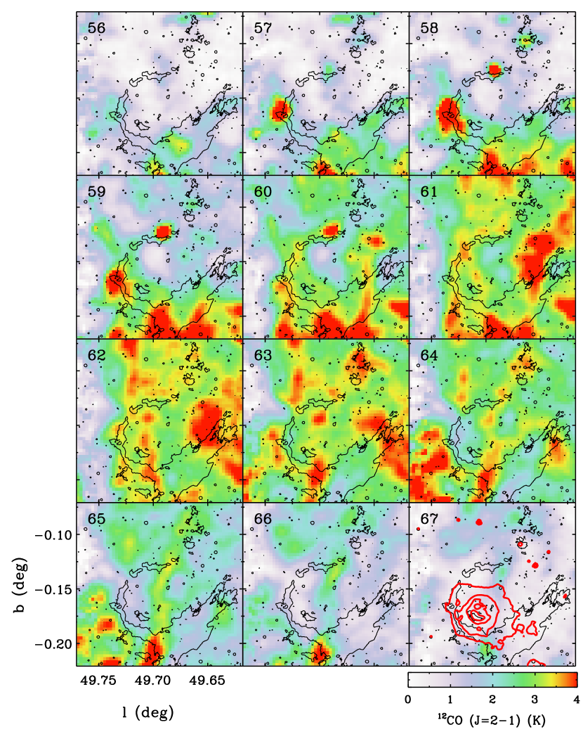
Figure 7.— The ¹²CO (J=2-1) channel maps by 1 km s^-1 interval. Black contour shows the shell structure of IRAC 8 $\micron$. Contour level is 50 MJy sr^-1. In last channel map, red contours are MIPS 24 $\micron$. Contour levels are 50, 100, 200, and 400 MJy sr^-1. The color scale bar is presented in units of K-T_MB.

To determine some physical properties of the shell structure, we used the ¹²CO (J=2-1), ¹³CO (J=2-1), and ¹³CO (J=1-0) maps described in Section 2. The first step is to determine the velocity range of the molecular components associated with the shell structure. Figure 5 (top) shows the velocity profile of each line averaged over the whole region shown in Figure 2. There are two bright components around 40 – 50 km s^-1 and 56 – 67 km s^-1 in the ¹³CO (J=2-1) line. We present the integrated intensity maps of ¹²CO (J=2-1) in two different velocity ranges in bottom of Figure 5.

In the ¹²CO (J=2-1) map integrated from 40 to 50 km s^-1 (Figure 5a), a strong component is located on the north-east side of the shell. Some bright emission is seen within the radius of N102. The ¹²CO (J=2-1) intensity map integrated from 56 to 67 km s^-1 (Figure 5b) shows that some clumpy structures surround the ionized region seen in the IRAC shell. We label two of these as clumps 1 and 2. The ¹²CO , ¹³CO (J=2-1) and ¹³CO (J=1-0) spectra around clump 1 and 2 are presented in Figure 6. Peak intensity of ¹²CO (J=2-1) appears around 59 km s^-1 in both clumps. The ¹³CO (J=2-1) line between 56 and 62 km s^-1 of clump 1 is very bright and distinguished from the other components in different velocity ranges. The ratio, ${{}^{12/13}R_{2-1}}$, of ¹²CO (J=2-1) and ¹³CO (J=2-1) at the peak velocity of ¹³CO (J=2-1) is 1.85 at the position marked as an asterisk in Figure 6 (left). In all spectra of clump 1 and 2, the main beam temperature of GRS ¹³CO (J=1-0) is brighter than the main beam temperature of HHT ¹³CO (J=2-1) implying the non-LTE state of shell region (§4.2).

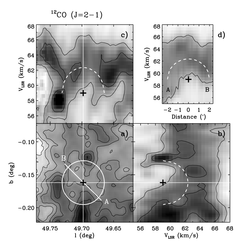
Figure 8.— ¹²CO spatial and position-velocity diagrams around the shell region. (a) is the ¹²CO (J=2-1) intensity map integrated between 55 and 68 km s^-1. Contour levels are 5, 10, 15, 20, 25, 30, 35, 40 and 45 K km s^-1. The cross symbol represents the center position of the N102 shell listed by Churchwell et al. (2006). White circle represents the shell size of 2 arcmin radius. The oblique line AB shows the section for the PV map presented in (d). (b) and (c) are position-velocity maps in latitude and longitude across the solid lines in (a). The contour levels are {1, 2, 4}$\times$1.6 K-T${}_{\mathrm{MB}}~{}(5\sigma)$. (d) A position-velocity diagram along AB. The x-axis is the distance from the center of the shell. Contour level is 1.6 K-T_MB. The velocity variation expected from equation (1), adopting $v_{0}$ = +3.4 km s^-1, $R$ = 2 arcmin, and $v_{sys}$ = +59 km s^-1, is shown by the dashed line.

Figure 7 shows ¹²CO (J=2-1) emission associated with the shell between 56 and 67 km s^-1 by 1 km s^-1 steps. The molecular and IRAC shells show good correspondence between 58 and 63 km s^-1 in the north-east quadrant where the shell is complete. To the north-west the shell is broken in both the IRAC and molecular line images. To the south the correspondence is less clear because of the presence of additional molecular gas extending off the map in Figure 7. MIPS 24 $\micron$ emission represented in the last channel, 67 km s^-1, fills the inside of the shell. The distribution of the CO molecular cloud agrees with the broken shell structure seen in IRAC bands. A molecular clump in the south forms the bright rim of the IRAC shell.

Figure 8 shows the spatial and kinematic structure around the shell in ¹²CO (J=2-1). Figure 8a is the ¹²CO (J=2-1) intensity integrated between 55 and 68 km s^-1. Figures 8b and 8c are position-velocity maps in latitude and longitude across the solid lines in Figure 8a, respectively. Figure 8d is the position-velocity map along a line $AB$ in the intensity map (Figure 8a). The cross represents the center position of the N102 shell. Although most CO emission is distributed broadly from 55 to 67 km s^-1, the shell structure is visible in the velocity range $V_{LSR}\simeq$ 56 to 62 km s^-1.

For a simple shell structure, the expected velocity along the line of sight can be expressed as

$$v(X)=v_{0}\sqrt{1-\frac{X^{2}}{R^{2}}}+v_{sys}$$ (3)

where $v_{0}$ is the expansion velocity, $R$ is the radius of the shell (2$\arcmin$) estimated from the IRAC images of N102, $X$ the projected distance from the center of the shell, and $v_{sys}$ the systematic LSR velocity of the whole system. We assume $v_{sys}=+59$ km s^-1 since all clumpy structures on the border of the shell show the peak at $v_{sys}=+59$. The expansion velocity of the shell is determined to be $v_{0}\simeq 3.4$ km s^-1 by least-squares fitting for the mean velocity within the shell radius. The expected velocity from equation (3) is presented as a dashed line. Although molecular material around the center of N102 has disappeared, especially toward north-west, molecular gas far from the central star still remains. The dynamical time-scale of N102 can be estimated by dividing the size, 2$\arcmin$, by the expansion velocity $v_{0}$. Assuming a $v_{sys}$ between 58 and 59 km s^-1 for N102, we estimate an age of 0.71 to 0.96 Myr for the derived expansion velocity, which varies from 3.4 km s^-1 to 4.5 km s^-1.

4.2. Physical Conditions

As mentioned in §4.1, the observed ratio of ¹³CO (J=2-1) and ¹³CO (J=1-0), ${}^{13}R_{2-1/1-0}$$\sim$ 0.5, shows that the shell region is not dense enough to satisfy the LTE condition. Considering the location of the shell region near the active star-forming complex, W51A, the kinetic temperature must be higher than 12K, derived from the maximum main beam temperature of ¹²CO (J=2-1). We therefore need to use a non-LTE statistical equilibrium treatment of the CO molecular excitation to study physical properties of the molecular cloud. We use the escape probability radiative transfer and photodissociation model of Kulesa et al. (2005), also described in Povich et al. (2009), to calculate grids of CO level populations for wide ranges of volume densities ($10^{2}-10^{7}$ cm^-3) and temperatures ($5-300$ K) assuming detailed balance and steady state. From these model grids, the total CO column density at each observed pixel is computed from the peak temperature, line widths and integrated intensities of the observed CO lines. Assuming that the CO heating is dominated by photon processes (e.g. the photoelectric heating of dust), a coarse estimate of the incident radiation field can be made for each point in the map. The photodissociation model is then applied to estimate a total hydrogen column density from the CO data. This calculation is based on the CO and H₂ photodissociation treatments of van Dishoeck & Black (1988) and Black & van Dishoeck (1987), respectively, using a total interstellar carbon abundance of $C/H=2.4\times 10^{-4}$ (Cardelli et al., 1996). Because the CO abundance is a strong function of column density, blind application of a uniform CO “dark cloud” abundance ($10^{-4}$) can lead to a gross underestimate of the total hydrogen column and gas mass. The visual extinction $A_{V}$, is calculated from $N(H)$ using $N(H)/A_{V}=1.9\times 10^{21}$ cm^-2 mag^-1 (Bohlin et al., 1978).

To determine how much molecular material is swept by the expanding H II region, we calculate the column density of CO between 56 and 62 km s^-1 centered on 59 km s^-1 . This range corresponds to the velocities that the clumps 1 and 2 on the shell occupy on the PV map (Figure 8).

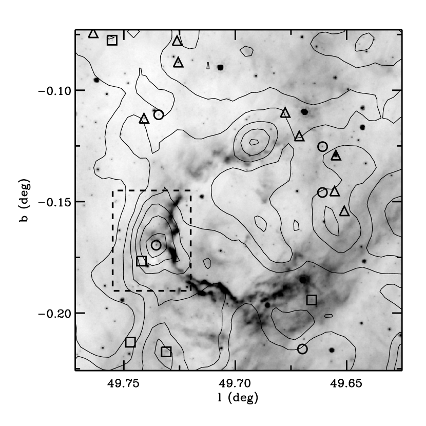
Figure 9.— Hydrogen column density contours superimposed on the IRAC 8.0 $\micron$ image (inverted grayscale). The hydrogen column density is integrated over the velocity range between 56 and 62 km s^-1. Contour levels are 40, 50, 60, 70, 80 and 90% of the peak hydrogen column density of $2.43\times 10^{22}$ cm^-2. YSO candidates are marked as circles for Stage 0/I, triangles for Stage II, and squares for ambiguous sources. The dashed box shows the region in Figure 10.

We apply this analysis to the combination of ¹³CO (J=1-0) data from GRS, and the ¹²CO (J=2-1) and ¹³CO (J=2-1) data from the HHT. We convolve all spectral line maps to the GRS resolution of 46″. From the escape probability model, we estimate a total mass of $3.2\times 10^{4}~{}{\rm M}_{\odot}$ distributed from 56 and 62 km s^-1 in the $0.152\arcdeg\times 0.150\arcdeg$ region shown in Figure 2.

To avoid degrading the resolution of our HHT maps, we also apply the non-LTE model to the ¹²CO (J=2-1) and ¹³CO (J=2-1) data. In this case, the total mass in the same velocity range and region is computed to be $2.9\times 10^{4}~{}{\rm M}_{\odot}$. The derived total mass from two lines of ¹²CO and ¹³CO (J=2-1) is $\sim$ 10% smaller than that derived from three lines of ¹²CO and ¹³CO (J=2-1) and ¹³CO (J=1-0). Since two results are similar, we present the total hydrogen column density $N(H)$ distribution derived from the HHT ¹²CO and ¹³CO (J=2-1) with 32″ spatial resolution in Figure 9.

5. Discussion

Using the CO data and the identified YSO candidates, we investigate whether our shell region are consistent with the predictions from the star formation triggered by the expansion of an H II region. Figure 9 shows the resulting distribution of the total hydrogen column density $N(H)$ with the shell structure on the IRAC 8 µm image. YSO candidates are indicated by circles for Stage 0/I, triangles for Stage II, and squares for ambiguous sources. Total hydrogen column density is derived from 56 to 62 km s^-1, which is the velocity range affected by the expansion of the H II region. Most dense condensations are distributed along the 8 µm shell. The distribution of the hydrogen in the inner region of the large shell is coincident with the distribution of the MIPS 24 µm emission encompassed by the IRAC 8 µm shell. The distribution of gas condensations along the 8 µm shell, including clump 1 and 2 (see Figure 5), supports that the molecular material collects on the boundary of the shell during the expansion of the H II region.

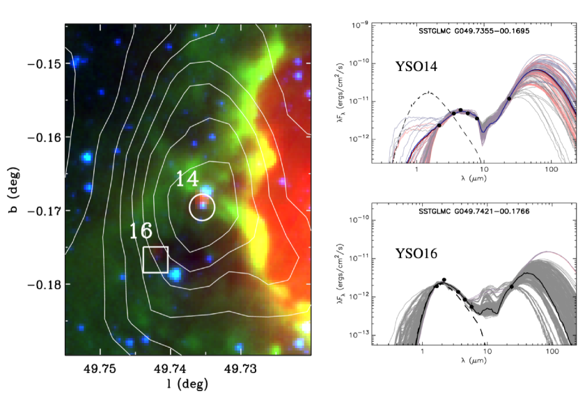
Figure 10.— $A_{V}$ contours superimposed on the composite image of MIPS 24 $\micron$ (red), IRAC 8.0 $\micron$ (green), and IRAC 4.5 $\micron$ (blue) of the dashed box region seen in Figure 9. Contour levels are {5, 6, 7, 8, 9, 10, 11, 12} mag. The candidate YSOs 14 and 16 are marked with circle (Stage 0/I) and square (Ambiguous). The SED model fits to the two sources are plotted on the right. The dashed curve shows the reddened photosphere of the central star.

According to the “collect and collapse” model (Elmegreen & Lada, 1977), a thin layer of compressed neutral material forms between the ionization front and the shock front as the H II region expands. This layer may become gravitationally unstable, fragment and form stars. Whitworth et al. (1994) have shown that the shell collected by the expansion of an H II region will fragment when its column density reaches $6\times 10^{21}$ cm^-2. Based on our escape probability model using the ¹²CO and ¹³CO (J=2-1) lines, the hydrogen column density of the most shell region is already greater than $1.0\times 10^{22}$ cm^-2 (the lowest contour in Figure 9 ; 40% of the peak hydrogen column density). Note that this $N(H)$ are a lower limit because the CO molecule may be depleted by freezeout onto dust grains. Therefore by the criterion of Whitworth et al. (1994), we conclude that the column density of the shell region is sufficient to form a new star by the collect and collapse process.

Dynamical expansion of the H II region has been simulated by Hosokawa & Inutsuka (2006). They describe the results of several models with different central stars (12 - 101 M_⊙) and ambient densities ($10^{2}-10^{4}$ cm^-3). We estimate that the N102 region has an O8.5V ionizing star with the ambient number density of about $10^{3}$ cm^-3, which we derive from $N(H)$ of $1.0\times 10^{22}$ cm^-2 and a line-of-sight depth of 2 pc, corresponding to the projected size of Clump 1. We compare the physical properties of N102 with the model S19 of Hosokawa & Inutsuka (2006) : central star mass of 19 M_⊙ with an ambient density of $10^{3}$ cm^-3. In this model, a star produces a shell of radius 3.5 pc after 1 Myr and an unstable region appears at about 0.5 Myr. For the N102 shell, the current radius of N102 is 3.3 pc at 5.7 kpc distance. Assuming a $V_{sys}$ of 59 km s^-1 for N102, we estimate an expansion velocity of 3.4 km s^-1 and an expansion time of 0.96 Myr. The shell size and the time scale are in excellent agreement with those of model S19 by Hosokawa & Inutsuka (2006). Therefore, we conclude that triggered star-formation on the border of N102 is possible by the expansion of the H II region.

Given that the accumulated molecular material is sufficient to form stars, we find two YSOs (14 and 16) associated with the Clump 1 that is the densest region along the shell structure. The hydrogen column density at the peak of clump 1 is $2.4\times 10^{22}$ cm^-2, corresponding to the visual extinction of $\sim 14$ mag. The mass of clump 1 shown in Figure 10 is $2.3\times 10^{3}$ M_⊙ based on the escape probability modeling using ¹²CO and ¹³CO (J=2-1) lines. This mass are lower limits because the CO molecule may be significantly depleted by freezeout onto dust grains in the core of the cloud.

Figure 10 shows the $A_{V}$ distribution of clump 1 on the MIPS 24 $\micron$ (red), IRAC 8.0 $\micron$ (green) and 4.5 $\micron$ (blue) composite images. YSO 14 and 16 are marked as a circle and square, respectively. YSO 14 and 16, classified as Stage 0/I and Ambiguous, lie close to the central region of clump 1. MIPS 24 $\micron$ emission fluxes of 94 and 15 mJy are detected from YSO 14 and 16. We also show the SED model fits to these source in Figure 10. YSO 14 is an intermediate YSO of $\sim 6$ M_⊙ with an accretion rate of $\sim 8\times 10^{-5}M_{\odot}~{}yr^{-1}$. YSO 16 has a mass of $\sim 3$ M_⊙ with an accretion rate of $\sim 1.6\times 10^{-5}M_{\odot}~{}yr^{-1}$. While YSO 16 is classified as an ambiguous stage, a early stage is indicated because the good-fit models include 62% (Stage 0/I), 20% (Stage II) and 18% (stage III).

If considering the total column density, age and size of the H II region predicted from the collect and collapse picture, star formation should be possible everywhere the material is collected on the border of the shell. As seen in Figure 9, although the CO emission is collected on the periphery along the IRAC shell, we cannot be sure whether all the YSOs seen in Figure 9 are associated with the material collected by the expansion of the H II region. At least, YSO 14 and 16 seem to be associated with the collected material directly. We conclude that those two YSOs have formed probably by the fragmentation of the collected material swept up by the expansion of the H II region.

It may be that the exciting star s8 which we have identified was itself formed by such a triggering process. The molecular gas in the shell has a very similar velocity to that of the gas associated with the W51A H II regions, so these clouds may be physically associated. If so, we may speculate that expansion of the ionized regions in W51A triggered the collapse leading to the formation of O-star s8 in a kind of sequential star formation.

6. Conclusions

We have studied triggered star formation near the multiple shells of N102 and N103 (Churchwell et al., 2006) using Spitzer IR and HHT CO observations. We have identified the candidate ionizing star (possibly O8.5V) of the double shell. The CO observations confirm that dense molecular material has been collected along the shell which has been detected in the Spitzer IRAC images. The CO distribution shows that the shell is blown out toward a lower density region to the northwest. We find two clumpy CO condensations with the same central velocity of 59 km s^-1 to the east and north along the edge of the IRAC shell. Total hydrogen column density around the shell is high enough to form new stars and we identify two YSOs in early stages (Stage 0/I) within the densest molecular clump 1. Using the CO position-velocity map, we find that the H II region is currently expanding with a velocity of 3.4 km s^-1, suggesting the shell’s expansion time of $\sim$ 1 Myr. This timescale is in good agreement with numerical simulations of the expansion of the H II region (Hosokawa & Inutsuka, 2006). We conclude that the star formation on the border of N102 is triggered by the expansion of the H II region.

References

- Altenhoff et al. (1979) Alternating, W. J., Downes, D., Pauls, T., & Schraml, J. 1979, A&AS, 35, 23
- Avedisova (2002) Avedisova, V. S. 2002,Astronomy Reports, 46, 193
- Bessell & Brett (1988) Bessell, M. S., & Brett, J. M. 1988, PASP, 100, 1134
- Benjamin et al. (2003) Benjamin, R. A., et al. 2003, PASP, 115, 953
- Benjamin et al. (2005) Benjamin, R. A., et al. 2005, ApJ, 630, L149
- Black & van Dishoeck (1987) Black, J. H., & van Dishoeck, E. F. 1987, ApJ, 322, 412
- Bohlin et al. (1978) Bohlin, R. C., Savage, B. D., & Drake, J. F. 1978, ApJ, 224, 132
- Brand & Blitz (1993) Brand, J., & Blitz, L. 1993,A&A, 275, 67
- Cardelli et al. (1996) Cardelli, J. A., Meyer, D. M., Jura, M., & Savage, B. D. 1996, ApJ, 467, 334
- Carey et al. (2005) Carey, S. J., et al. 2005, Bulletin of the American Astronomical Society, 37, 1252
- Churchwell et al. (2006) Churchwell, E., et al. 2006, ApJ, 649, 759
- Churchwell et al. (2009) Churchwell, E., et al. 2009, PASP, 121, 213
- Condon et al. (1998) Condon, J. J., Cotton, W. D., Greisen, E. W., Yin, Q. F., Perley, R. A., Taylor, G. B., & Broderick, J. J. 1998, AJ, 115, 1693
- Deharveng et al. (2003) Deharveng, L., Lefloch, B., Zavagno, A., Caplan, J., Whitworth, A. P., Nadeau, D., & Martín, S. 2003, A&A, 408,L25
- Elmegreen & Lada (1977) Elmegreen, B. G., & Lada, C. J. 1977, ApJ, 214, 725
- Evans et al. (2009) Evans, N., et al. 2009, arXiv:0901.1691
- Fazio et al. (2004) Fazio, G. G., et al. 2004, ApJS, 154, 10
- Gregory et al. (1996) Gregory, P. C., Scott, W. K., Douglas, K., & Condon, J. J. 1996, ApJS, 103, 427
- Hosokawa & Inutsuka (2006) Hosokawa, T., & Inutsuka, S.-i. 2006, ApJ, 646, 240
- Indebetouw et al. (2005) Indebetouw, R., et al. 2005, ApJ, 619, 931
- Kim et al. (2007) Kim, H., Nakajima, Y., Sung, H., Moon, D.-S., & Koo, B.-C. 2007, Journal of Korean Astronomical Society, 40, 17
- Koo & Moon (1997) Koo, B.-C., & Moon, D.-S. 1997, ApJ, 475, 194
- Koornneef (1983) Koornneef, J. 1983, A&A, 128, 84
- Kulesa et al. (2005) Kulesa, C. A., Hungerford, A. L., Walker, C. K., Zhang, X., & Lane, A. P. 2005, ApJ, 625, 194
- Kutner & Ulich (1981) Kutner, M. L., & Ulich, B. L. 1981, ApJ, 250, 341
- Martins et al. (2005) Martins, F., Schaerer, D., & Hillier, D. J. 2005, A&A, 436, 1049
- Okumura et al. (2000) Okumura, S.-i., Mori, A., Nishihara, E., Watanabe, E., & Yamashita, T. 2000, ApJ, 543, 799
- Pomarès et al. (2009) Pomarès, M., et al. 2009, A&A, 494, 987
- Povich et al. (2009) Povich, M. S., et al. 2009, ApJ, 696, 1278
- Rieke et al. (2004) Rieke, G. H., et al. 2004, ApJS, 154, 25
- Robitaille et al. (2006) Robitaille, T. P., Whitney, B. A., Indebetouw, R., Wood, K., & Denzmore, P. 2006, ApJS, 167, 256
- Robitaille et al. (2007) Robitaille, T. P., Whitney, B. A., Indebetouw, R., & Wood, K. 2007, ApJS, 169, 328
- Sault et al. (1995) Sault, R. J.,Teuben, P. J., & Wright, M. C. H. 1995, Astronomical Data Analysis Software and Systems IV, 77, 433
- Simpson & Rubin (1990) Simpson, J. P., & Rubin, R. H. 1990, ApJ, 354, 165
- Skrutskie et al. (2006) Skrutskie, M. F., et al. 2006, AJ, 131, 1163
- Taylor et al. (1996) Taylor, A. R., Goss, W. M., Coleman, P. H., van Leeuwen, J., & Wallace, B. J. 1996, ApJS, 107, 239
- Watson et al. (2008) Watson, C., et al. 2008, ApJ, 681, 1341
- Whitworth et al. (1994) Whitworth, A. P., Bhattal, A. S., Chapman, S. J., Disney, M. J., & Turner, J. A. 1994, MNRAS, 268, 291
- Wink et al. (1982) Wink, J. E., Altenhoff, W. J., & Mezger, P. G. 1982, A&A, 108, 227
- van Dishoeck & Black (1988) van Dishoeck, E. F., & Black, J. H. 1988, ApJ, 334, 771
- Zavagno et al. (2006) Zavagno, A., Deharveng, L., Comerón, F., Brand, J., Massi, F., Caplan, J., & Russeil, D. 2006, A&A, 446, 171