Full Quantum Analysis of Two-Photon Absorption Using Two-Photon Wavefunction: Comparison with One-Photon Absorption

Abstract

For dissipation-free photon-photon interaction at the single photon level, we analyze one-photon transition and two-photon transition induced by photon pairs in three-level atoms using two-photon wavefunctions. We show that the two-photon absorption can be substantially enhanced by adjusting the time correlation of photon pairs. We study two typical cases: Gaussian wavefunction and rectangular wavefunction. In the latter, we find that under special conditions one-photon transition is completely suppressed while the high probability of two-photon transition is maintained.

1 Introduction

Two-photon absorption is one of the most fundamental nonlinear processes, and it sometimes reveals the quantum nature of light [1]. If a two-photon transition is achieved at a single-photon level, it can be possible to control the fate of a single photon by controlling the presence or absence of the other single photon. Such photon-photon interaction may be applicable to quantum information technologies, such as the development of optical switches for two photons and Bell-state analyzers [2] among others. [3, 4, 5, 6, 7, 8]. In these applications, the medium must be such that it absorbs the two photons and not one of them. In three-level systems having a ground state, intermediate state, and an excited state, two-photon absorption and one-photon absorption to the intermediate level can occur simultaneously. The two-photon absorption can be enhanced by decreasing the detuning to the intermediate state; however, this may also result in an increase in the one-photon transitions to the intermediate level. Several methods for enhancing the two-photon absorption while suppressing the one-photon absorption have been proposed. The use of electromagnetically induced transparency (EIT) is one approach for realizing the suppression of one-photon transition while maintaining the strong nonlinearity in four-level atoms using auxiliary light called the coupling light [9, 10, 11]. The cavity QED is another promising method for obtaining effective two-photon absorption [12].

It is also possible to enhance two-photon absorption by tailoring the quantum state of photons [13, 14]; this does not involve the use of any external apparatus such as a cavity or a control light, as in the case of the EIT system. To obtain efficient two-photon excitations, the two photons must satisfy the following two conditions: they should be close to each other, and the total linewidth of the two photons (two-photon linewidth) must be less than the linewidth of the excited state. Satisfying the first condition enables the occurrence of instantaneous transition via the virtual state, and the second one ensures that two-photon resonance occurs for a long time. An ultrashort light pulse does not satisfy the second condition because of its broad spectrum. In contrast, twin photons produced by spontaneous parametric down-conversion (SPDC) processes using a continuous pump laser satisfy both the conditions and can effectively undergo two-photon transitions. However, the suppression of the one-photon transitions to the intermediate state and enhancement of the two-photon transitions have not been investigated in detail.

In order to evaluate the transition probabilities of photon pairs, full quantum treatment of the system is required. We consider a propagating light beam consisting of continuous modes, which requires a multimode description. To carry out the full quantum multimode analysis of this light beam, we introduce two-photon wavefunctions that can represent arbitrary two-photon states [15, 16, 17, 18, 19]. Our formulation allows us to analytically estimate not only two-photon absorption but also the one-photon absorption.

In Sec. 2, we describe the formulation both the two-photon and one-photon absorption for arbitrary two-photon states using two-photon wavefunction. In Sec. 3, we compare the two-photon and one-photon absorptions for two types of time-correlated photon pairs. Finally, we show that by adjusting the correlation time, the single-photon loss can be suppressed without decreasing the high probability of two-photon absorption.

2 Theory

2.1 Field operators in free space

\psfrag{wi}[c][c]{$\omega_{i}$}\psfrag{w}[c][c]{$\omega$}\psfrag{W}[c][c]{$\Omega$}\psfrag{Wi}[c][c]{$\Omega_{i}$}\psfrag{W1}[c][c]{$\Omega_{a}$}\psfrag{W2}[c][c]{$\Omega_{b}$}\psfrag{w1}[c][c]{$\omega_{1}$}\psfrag{w2}[c][c]{$\omega_{2}$}\psfrag{g}[c][c]{$|g\rangle$}\psfrag{a}[c][c]{$|a\rangle$}\psfrag{b}[c][c]{$|b\rangle$}\psfrag{e}[c][c]{$|e\rangle$}\includegraphics[width=199.16928pt]{level.eps}

Figure 1: Level diagrams for (a) one-photon transition and (b) two-photon transition.

In order to investigate the interaction of atoms with an electromagnetic field propagating in one dimension, we define the electric field in continuous modes as

$$\hat{E}(z,t)=\int^{\infty}_{-\infty}{\mathrm{d}}\omega\sqrt{\frac{\hbar\omega}{4\pi\epsilon_{0}cA}}\hat{a}(\omega)\,{\mathrm{e}}^{-{\mathrm{i}}\omega(t-z/c)}+{\rm H.c.},$$ (1)

where $A$ denotes the cross section of the beam [15]. The annihilation operator $\hat{a}(\omega)$ satisfies the following commutation relation:

$$[\hat{a}(\omega),\hat{a}^{\dagger}(\omega^{\prime})]=\delta(\omega-\omega^{\prime}).$$ (2)

If the bandwidth of the field is assumed to be considerably less than the carrier frequency $\bar{\omega}$, we can simplify eq. (1) as

$$\hat{E}(z,t) =\mathcal{E}\,\hat{a}(t-z/c)+{\rm H.c.},$$ (3)

where

$$\hat{a}(t) \equiv\frac{1}{\sqrt{2\pi}}\int^{\infty}_{-\infty}{\mathrm{d}}\omega\,\hat{a}(\omega)\,{\mathrm{e}}^{-{\mathrm{i}}\omega t},$$ (4)

$$\mathcal{E} \equiv\sqrt{\frac{\hbar\bar{\omega}}{2\epsilon_{0}cA}}.$$ (5)

The Fourier transformed operator $\hat{a}(t)$ has the same commutation relation as $\hat{a}(\omega)$:

$$[\hat{a}(t),\hat{a}^{\dagger}(t^{\prime})]=\delta(t-t^{\prime}).$$ (6)

2.2 Single-photon transition

Before discussing the two-photon transitions, we first consider the interaction between a wavepacket containing a single photon and a two-level atom, as shown in Fig. 1(a). The initial state of the single-photon wavepacket is represented as $|\psi\rangle$, and the atom at $z=0$ is prepared in the ground state $|g\rangle$. We introduce a simplified notation $|g,\psi\rangle=|g\rangle|\psi\rangle$ to represent the composite system. The Hamiltonian in the interaction picture is

$$\hat{H}(t)=\hat{p}(t)\hat{E}(t),$$ (7)

where

$$\hat{p}(t) =\mathcal{P}|e\rangle\langle g|{\mathrm{e}}^{{\mathrm{i}}\Omega t}+{\rm H.c.}$$ (8)

represents an atomic dipole oscillating at the transition frequency $\Omega$ and the electric-dipole transition matrix element given as $\mathcal{P}=-e\langle e|r|g\rangle$ [16].

By applying the first-order perturbation theory, the probability amplitude for the atom to exist in the excited state $|e\rangle$ after the passage of the wavepacket is given as

$$\alpha_{1}=-\frac{{\mathrm{i}}}{\hbar}\int^{\infty}_{-\infty}{\mathrm{d}}t\langle e,0|\hat{H}(t)|g,\psi\rangle,$$ (9)

where $|e,0\rangle=|e\rangle|0\rangle$ with the vacuum state $|0\rangle$. We assume that the transit time of the wavepacket is shorter than the relaxation time of the excited state $|e\rangle$. On substituting eqs. (3) and (7) in eq. (9), we obtain

$$\alpha_{1}=-\frac{{\mathrm{i}}\mathcal{E}\mathcal{P}}{\hbar}\int^{\infty}_{-\infty}{\mathrm{d}}t\,{\mathrm{e}}^{{\mathrm{i}}\Omega t}\langle 0|\hat{a}(t)|\psi\rangle.$$ (10)

In this derivation, we use the rotating wave approximation. We introduce the one-photon amplitude

$$\psi(t)\equiv\langle 0|\hat{a}(t)|\psi\rangle,$$ (11)

whose square is proportional to the probability of photon detection at time $t$ [16]. Its Fourier transform is expressed as

$$\Psi(\omega)=\frac{1}{\sqrt{2\pi}}\int^{\infty}_{-\infty}{\mathrm{d}}t\,\psi(t)\,{\mathrm{e}}^{{\mathrm{i}}\omega t},$$ (12)

the square of which represents the spectral intensity of the wavepacket; then, the probability of excitation, $P_{1}\equiv|\alpha_{1}|^{2}$, can be expressed as

$$P_{1} =2\pi r|\Psi(\Omega)|^{2},$$ (13)

where $r\equiv\mathcal{E}^{2}\mathcal{P}^{2}/\hbar^{2}$. Thus, the probability of the one-photon absorption is determined by the spectral component $|\Psi(\Omega)|^{2}$ at the atomic transition frequency of $\Omega$.

2.3 Two-photon transition

In this section, we discuss the two-photon transitions induced by a pair of photons, as shown in Fig. 1 (b). Let us consider that photon 1 in a mode induces the lower transition, $|g\rangle\rightarrow|a\rangle$ while photon 2 in another mode is responsible for the upper transition, $|a\rangle\rightarrow|b\rangle$.

The interaction Hamiltonian for this scenario is represented as

$$\hat{H}(t) =\hat{p}_{1}(t)\hat{E}_{1}(t)+\hat{p}_{2}(t)\hat{E}_{2}(t),$$ (14)

where

$$\hat{p}_{1}(t) =\mathcal{P}_{a}|a\rangle\langle g|{\mathrm{e}}^{{\mathrm{i}}\Omega_{a}t}+{\rm H.c.},$$ (15)

$$\hat{p}_{2}(t) =\mathcal{P}_{b}|b\rangle\langle a|{\mathrm{e}}^{{\mathrm{i}}\Omega_{b}t}+{\rm H.c.}$$ (16)

To estimate the two-photon excitation probability, we use the second-order perturbation theory. The second-order component of the time evolution operator is expressed as

$$\hat{U}_{2} =-\frac{1}{\hbar^{2}}\int^{\infty}_{-\infty}\int^{\infty}_{-\infty}{\mathrm{d}}t_{2}{\mathrm{d}}t_{1}\hat{H}(t_{2})\hat{H}(t_{1})\,\theta(t_{2}-t_{1}),$$ (17)

where $\theta(t)$ is the Heaviside step function:

$$\theta(t)=\begin{cases}1&(t\geq 0),\\ 0&(t<0).\end{cases}$$ (18)

When a wavepacket $|\psi\rangle$, containing a pair of photons, passes through an atom in the ground state $|g\rangle$, the probability amplitude of the two-photon excitation can be given as

$$\alpha_{2} =\langle b,0|\hat{U}_{2}|g,\psi\rangle$$

$$=-\frac{\mathcal{E}_{1}\mathcal{E}_{2}\mathcal{P}_{a}\mathcal{P}_{b}}{\hbar^{2}}\int^{\infty}_{-\infty}\int^{\infty}_{-\infty}{\mathrm{d}}t_{2}{\mathrm{d}}t_{1}{\mathrm{e}}^{{\mathrm{i}}\Omega_{b}t_{2}}{\mathrm{e}}^{{\mathrm{i}}\Omega_{a}t_{1}}$$

$$\hskip 28.45274pt\times\langle 0|\hat{a}_{2}(t_{2})\hat{a}_{1}(t_{1})|\psi\rangle\,\theta(t_{2}-t_{1}).$$ (19)

Similar to the case of eq. (11), we can define the two-photon amplitude as

$$\psi(t_{1},t_{2})=\langle 0|\hat{a}_{2}(t_{2})\hat{a}_{1}(t_{1})|\psi\rangle,$$ (20)

whose square corresponds to the joint probability of finding photon 1 at $t=t_{1}$ and photon 2 at $t=t_{2}$. The above two-photon amplitude is called an effective two-photon wavefunction or a biphoton [20, 17]. It is clear that the part of $\psi(t_{1},t_{2})$ for $t_{2}<t_{1}$ does not contribute to the two-photon excitation because the absorption of photon 1 is always followed by that of photon 2. In addition to the Fourier transform of $\psi(t_{1},t_{2})$, which is given as

$$\Psi(\omega_{1},\omega_{2}) \equiv\frac{1}{2\pi}\int^{\infty}_{-\infty}\int^{\infty}_{-\infty}{\mathrm{d}}t_{2}\,{\mathrm{d}}t_{1}\,$$

$$\times{\mathrm{e}}^{{\mathrm{i}}\omega_{2}t_{2}}{\mathrm{e}}^{{\mathrm{i}}\omega_{1}t_{1}}\psi(t_{1},t_{2}),$$ (21)

we also introduce the Fourier transform of $\psi(t_{1},t_{2})\theta(t_{2}-t_{1})$:

$$\tilde{\Psi}(\omega_{1},\omega_{2}) \equiv\frac{1}{2\pi}\int^{\infty}_{-\infty}\int^{\infty}_{-\infty}{\mathrm{d}}t_{2}\,{\mathrm{d}}t_{1}\,$$

$$\ \times{\mathrm{e}}^{{\mathrm{i}}\omega_{2}t_{2}}{\mathrm{e}}^{{\mathrm{i}}\omega_{1}t_{1}}\psi(t_{1},t_{2})\theta(t_{2}-t_{1});$$ (22)

this Fourier transform represents the spectral intensity of the photon pair under the time ordering $t_{2}>t_{1}$. From eq. (19), we derive the probability of two-photon excitation, $P_{2}=|\alpha_{2}|^{2}$, as

$$P_{2}=4\pi^{2}r_{1}r_{2}|\tilde{\Psi}(\Omega_{a},\Omega_{b})|^{2},$$ (23)

where $r_{1}\equiv\mathcal{E}_{1}^{2}\mathcal{P}_{a}^{2}/\hbar^{2}$ and $r_{2}\equiv\mathcal{E}_{2}^{2}\mathcal{P}_{b}^{2}/\hbar^{2}$. The probability of two-photon absorption is given by the spectral component $|\tilde{\Psi}(\Omega_{a},\Omega_{b})|^{2}$ of the time-ordered wavefunction at the transition frequencies of $\Omega_{a}$ and $\Omega_{b}$.

2.4 One-photon transition induced by one photon of the photon pair

In this section, we consider the probability $P_{1}$ of photon 1 exciting the atom to the intermediate level $|a\rangle$. In eq. (13), the probability of one-photon absorption is determined by the spectrum of the photon that induces the transition. If the two photons are not entangled, i. e. , $\Psi(\omega_{1},\omega_{2})=\Psi_{1}(\omega_{1})\otimes\Psi_{2}(\omega_{2})$, we can easily derive the excitation probability as $P_{1}=2\pi r_{1}|\Psi_{1}(\Omega_{a})|^{2}$. However, in the case of an entangled photon, shown in Fig. 2(a), the spectrum of photon 1 cannot be represented as the function of $\omega_{1}$ alone, because the spectrum of photon 1 depends on that of photon 2. In such cases, the probability of one-photon absorption is obtained by tracing over the state of photon 2 as

$$P_{1}=2\pi r_{1}\int^{\infty}_{-\infty}{\mathrm{d}}\omega_{2}^{\prime}|\Psi(\Omega_{a},\omega_{2}^{\prime})|^{2}.$$ (24)

\psfrag{omega1}[c][c]{$\omega_{1}$}\psfrag{omega2}[c][c]{$\omega_{2}$}\psfrag{omegaa}[c][c]{$\Omega_{a}$}\psfrag{omegab}[l][l]{$\Omega_{b}$}\psfrag{omegaab}[c][c]{$\bar{\omega}_{1}$}\psfrag{omegabb}[l][l]{$\bar{\omega}_{2}$}\psfrag{delta}[c][l]{$\Delta$}\psfrag{tau}[c][l]{$1/\tau$}\psfrag{T}[c][l]{$1/T$}\psfrag{spectrum1}[l][l]{$|\Psi(\omega_{1},\omega_{2})|$}\psfrag{spectrum2}[l][l]{$|\tilde{\Psi}(\omega_{1},\omega_{2})|$}\includegraphics[width=199.16928pt]{spectrum.eps}

Figure 2: Schematic diagram of (a) $|\Psi(\omega_{1},\omega_{2})|$ and (b) $|\tilde{\Psi}(\omega_{1},\omega_{2})|$

3 Two-photon absorption induced by time-correlated photon pairs

Before introducing the two-photon wavefuction specific to this study, we will discuss the general properties of two-photon absorption induced by a time-correlated photon pair. The two-photon wavefunction is characterized by two parameters: coherent time $T$ and correlation time $\tau$. The coherence time $T$ is equal to the coherence time of the pump field. The correlation time $\tau\,(\ll T)$ corresponds to the time period required for both the photons to be detected by the two detectors and is determined by the spectral width of the down-converted light. In the frequency domain, the two-photon wavefunction $\Psi(\omega_{1},\omega_{2})$ can be represented as the product of two functions: $\Psi_{+}(\omega_{+})$ with a width of $1/T$ and $\Psi_{-}(\omega_{-})$ with a width of $1/\tau$ , where $\omega_{+}\equiv\omega_{1}+\omega_{2}$ and $\omega_{-}\equiv(\omega_{1}-\omega_{2})/2$, as shown in Fig. 2(a). From eq. (22), $\tilde{\Psi}(\omega_{1},\omega_{2})$ is represented as the convolution integral:

$$\tilde{\Psi}(\omega_{1},\omega_{2})=\Psi_{+}(\omega_{+})\int{\mathrm{d}}\omega_{-}^{\prime}\Psi_{-}(\omega_{-}-\omega_{-}^{\prime})\Theta(\omega_{-}^{\prime}),$$ (25)

where $\Theta(\omega)$ is the Fourier integral of the Heaviside step function $\theta(t)$ and is given by

$$\Theta(\omega)=\sqrt{\frac{\pi}{2}}\delta(\omega)-\frac{{\mathrm{i}}}{\sqrt{2\pi}}\frac{\rm P}{\omega}.$$ (26)

The symbol ${\rm P}$ denotes the Cauchy principal value [21]. The second term in the above equation causes the spectrum of ${\Psi}(\omega_{1},\omega_{2})$ to broaden in the direction of the frequency difference $\omega_{-}$, as shown in Fig. 2(b), because of its convolution integral with $1/\omega$.

For simplicity, it is assumed that

$$\Psi_{+}(\omega_{+}) =\frac{\beta}{\sqrt{T}}\phi((\omega_{+}-\bar{\omega}_{+})T)$$

$$\Psi_{-}(\omega_{-}) =\frac{\beta}{\sqrt{\tau}}\phi((\omega_{-}-\bar{\omega}_{-})\tau),\quad$$ (27)

where the common function $\phi(\alpha\omega)$, which satisfies $\int\phi(\alpha\omega){\mathrm{d}}\omega=1$, has a width of $1/\alpha$, height of $\alpha$, and shows a peak at $\bar{\omega}_{\pm}$. (The coefficient $\beta$ must be determined to satisfy the normalization condition $\int{\mathrm{d}}\omega_{\pm}|\Psi_{\pm}(\omega_{\pm})|^{2}=1$.) When the two-photon-resonance condition is satisfied as $\bar{\omega}_{+}=\Omega_{+}(\equiv\Omega_{a}+\Omega_{b})$, we get ${\Psi}_{+}(\Omega_{+})=\beta\phi(0)/\sqrt{T}=\beta\sqrt{T}$. If the detuning $\Delta$ is sufficiently large for $\phi((\omega_{-}-\bar{\omega}_{-})\tau)$ to be regarded as a delta function, we can obtain

$$\tilde{\Psi}(\Omega_{a},\Omega_{b})\propto\sqrt{\frac{T}{\tau}}\frac{1}{\Delta},\quad P_{2}\propto\frac{T}{\tau}\frac{1}{\Delta^{2}},$$ (28)

where $\Delta\equiv(\Omega_{a}-\Omega_{b})/2-\bar{\omega}_{-}$ corresponds to the detuning from the intermediate state. It should be noted that the two-photon absorption probability scales as $P_{2}\propto 1/\Delta^{2}$. This result is consistent with the fact that two-photon processes via a virtual state are a function of $1/\Delta^{2}$, which is derived for two cavity modes [22]. Equation (28) also indicates that the time correlation $\tau\ll T$, which is a unique property of time-correlated photon pairs, substantially enhances the two-photon absorption probability $P_{2}$.

Next, we compare the probability of two-photon excitation, $P_{2}$, with that of one-photon excitation to the intermediate state $|a\rangle$, $P_{1}$, for the incidence of a photon pair. For any two-photon wavepacket, we can calculate $P_{2}$ and $P_{1}$ using eq. (23) and eq. (24), respectively. The probabilities $P_{1}$ and $P_{2}$ are significantly affected by the shape of the two-photon wavefunction, as described in Sec. 2. In the following subsections, we investigate these probabilities in two cases: the case of a Gaussian wavefunction, as shown in Fig. 3(a), and the case of a rectangular wavefunction, as shown in Fig. 3(b). The Gaussian wavefunction can be obtained by restricting the spectrum of photon pairs using a Gaussian filter. The rectangular wavefunction can be generated by a photon pairs via type-II spontaneous parametric-down conversion due to the difference in group velocities of two photons [17, 15].

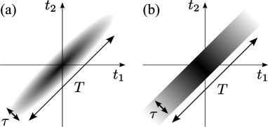
Figure 3: Two-photon wavefunction: (a) Gaussian and (b) rectangular.

3.1 Gaussian wavefunction

The Gaussian two-photon wavefunction is represented as

$$\psi(t_{1},t_{2})=a_{1} {\mathrm{e}}^{-(t_{1}+t_{2})^{2}/16T^{2}}{\mathrm{e}}^{-(t_{1}-t_{2})^{2}/4\tau^{2}}$$

$$\times{\mathrm{e}}^{-{\mathrm{i}}\bar{\omega}_{1}t_{1}}{\mathrm{e}}^{-{\mathrm{i}}\bar{\omega}_{2}t_{2}},$$ (29)

where $\bar{\omega}_{1}$ ($\bar{\omega}_{2}$) is the central frequency of the signal (idler) photon and $a_{1}=1/\sqrt{2\pi\tau T}$ is the normalization factor. The Fourier transform of this wavefunction is easily derived as

$$\Psi(\omega_{1},\omega_{2})=A_{1}{\mathrm{e}}^{-(\omega_{+}-\bar{\omega}_{+})^{2}T^{2}}\,{\mathrm{e}}^{-(\omega_{-}-\bar{\omega}_{-})^{2}\tau^{2}},$$ (30)

where $A_{1}=\sqrt{2\tau T/\pi}$. From its definition given in eq. (22), we obtain

$$\tilde{\Psi}(\omega_{1},\omega_{2})=\frac{A_{1}}{2}{\mathrm{e}}^{-(\omega_{+}-\bar{\omega}_{+})^{2}T^{2}}\,F\left((\omega_{-}-\bar{\omega}_{-})\tau\right),$$ (31)

where $F(\xi)$ is called plasma dispersion function [23] and defined as

$$F(\xi)={\mathrm{e}}^{-\xi^{2}}\left(1+\frac{2{\mathrm{i}}}{\sqrt{\pi}}\int^{\xi}_{0}{\mathrm{e}}^{y^{2}}{\mathrm{d}}y\right).$$ (32)

It should be noted that the Gauss function in the last factor of eq. (30) is replaced with the plasma dispersion function in eq. (31).

By substituting eq. (31) in eq. (23) and assuming that the sum of the two-photon frequency is tuned to the two-photon transition, i.e., $\bar{\omega}_{+}=\Omega_{a}+\Omega_{b}$, we obtain the probability of the two-photon transition as

$$P_{2}=\pi^{2}r_{1}r_{2}A_{1}^{2}\,|F(\Delta\cdot\tau)|^{2}.$$ (33)

From eqs. (30) and (23), the probability of the one-photon transition to the intermediate state $|a\rangle$ can be derived as

$$P_{1} =2\pi r_{1}A_{1}^{2}\int^{\infty}_{-\infty}{\mathrm{d}}\omega_{2}$$

$$\hskip 28.45274pt\times{\mathrm{e}}^{-2(\omega_{2}-\Omega_{b})^{2}T^{2}}\,{\mathrm{e}}^{-(2\Delta-\omega_{2}+\Omega_{b})^{2}\tau^{2}/2}$$

$$=\frac{\sqrt{2}\pi^{3/2}r_{1}A_{1}^{2}}{T}{\mathrm{e}}^{-2(\Delta\cdot\tau)^{2}}$$ (34)

In the above derivation, we assume that $T\gg\tau$, which allows us to consider ${\mathrm{e}}^{-2(\omega_{2}-\Omega_{b})^{2}T^{2}}$ as the delta function $\sqrt{\pi/2}\,\delta(\omega_{2}-\Omega_{b})/T$.

Here, we introduce the ratio

$$R_{G}\equiv\frac{P_{2}}{P_{1}}=\sqrt{\frac{\pi}{2}}r_{2}T\,\cdot\,\frac{|F(\Delta\cdot\tau)|^{2}}{{\mathrm{e}}^{-2(\Delta\cdot\tau)^{2}}}.$$ (35)

In the second factor, which is a function of the correlation time $\tau$, both the Gauss function ${\mathrm{e}}^{-2(\Delta\cdot\tau)^{2}}$ in the numerator and the square of the plasma dispersion function $|F(\Delta\cdot\tau)|^{2}$ in the denominator are monotonously decreasing functions, as shown in Fig. 4(a). However, there exists a critical difference in the asymptotic behavior of $\Delta\cdot\tau>1$: ${\mathrm{e}}^{-2(\Delta\cdot\tau)^{2}}$ decreases rapidly, while $|F(\Delta\cdot\tau)|^{2}$ decreases slowly as $1/(\Delta\tau)^{2}$. Hence, we expect that the two-photon transition probability $P_{2}$ exceeds the one-photon transition probability $P_{1}$ depending on the value of $\Delta$ and selected $\tau$, even if the first factor in eq. (35) is less than 1.

\psfrag{f1}[c][c]{$|F(\Delta\cdot\tau)|^{2},\ {\mathrm{e}}^{-2(\Delta\cdot\tau)^{2}}$}\psfrag{f2}[c][c]{${\rm sinc}^{2}(\Delta\cdot\tau/2),\ {\rm sinc}^{2}(\Delta\cdot\tau)$}\psfrag{time}[c][c]{ correlation time $\Delta\cdot\tau$}\includegraphics[width=142.26378pt]{P1vsP2.eps}

Figure 4: (a) Comparison of $|F(\Delta\cdot\tau)|^{2}$ (solid line) with ${\mathrm{e}}^{-2(\Delta\cdot\tau)^{2}}$ (dashed line). (b) Comparison of ${\rm sinc}^{2}(\Delta\cdot\tau/2)$ (solid line) with ${\rm sinc}^{2}(\Delta\cdot\tau)$ (dashed line).

3.2 Rectangular wavefunction

By performing the type-II spontaneous parametric-down conversion and using a birefringent crystal to achieve group velocity compensation, we prepare the two-photon wavefunction, which is expressed as

$$\psi(t_{1},t_{2})=a_{2} \,{\mathrm{e}}^{-(t_{1}+t_{2})^{2}/16T^{2}}$$

$$\times\Pi_{\tau}(t_{1}-t_{2}){\mathrm{e}}^{-{\mathrm{i}}\bar{\omega}_{1}t_{1}}\,{\mathrm{e}}^{-{\mathrm{i}}\bar{\omega}_{2}t_{2}},$$ (36)

where $\Pi_{\tau}(t)$ is a window function defined as

$$\Pi_{\tau}(t)=\begin{cases}0&(|t|>\tau),\\ 1&(|t|<\tau),\end{cases}$$ (37)

and the normalization constant is $a_{2}=1/(8\pi)^{1/4}/\sqrt{\tau T}$ [17, 20].

As shown in Sec. 3.1, we can deduce $\Psi(\omega_{1},\omega_{2})$ and $\tilde{\Psi}(\omega_{1},\omega_{2})$ as follows:

$$\Psi(\omega_{1},\omega_{2}) =A_{2}\,{\mathrm{e}}^{-(\omega_{+}-\bar{\omega}_{+})T^{2}}\,{\rm sinc}\left((\omega_{-}-\bar{\omega}_{-})\tau\right)$$ (38)

$$\tilde{\Psi}(\omega_{1},\omega_{2}) =\frac{A_{2}}{2}\,{\mathrm{e}}^{-(\omega_{+}-\bar{\omega}_{+})T^{2}}\,$$

$$\times{\rm sinc}\left(\frac{\omega_{-}-\bar{\omega}_{-}}{2}\tau\right){\mathrm{e}}^{{\mathrm{i}}(\omega_{-}-\bar{\omega}_{-})\tau/2},$$ (39)

where ${\rm sinc}\,x\equiv\sin x/x$ and $A_{2}=(2/\pi^{3})^{1/4}\sqrt{\tau T}$. On substituting eqs. (38) and (39) in eqs. (23) and (24), respectively, we obtain

$$P_{1} =\frac{\sqrt{2}\pi^{3/2}r_{1}A_{2}^{2}}{T}\,{\rm sinc^{2}}\left(\Delta\cdot\tau\right),$$ (40)

$$P_{2} =\pi^{2}r_{1}r_{2}A_{2}^{2}\,{\rm sinc^{2}}\left(\frac{\Delta\cdot\tau}{2}\right).$$ (41)

Then, the ratio $R_{r}$ is given as

$$R_{r}\equiv\frac{P_{2}}{P_{1}}=\sqrt{\frac{\pi}{2}}r_{2}T\,\cdot\,\frac{{\rm sinc^{2}}\left(\frac{\Delta\cdot\tau}{2}\right)}{{\rm sinc^{2}}(\Delta\cdot\tau)}.$$ (42)

The first factor in this equation is identical to that in eq. (35) because the two wavefunctions expressed in eqs. (29) and (36) exhibit the same function with respect to $t_{1}+t_{2}$. In the second factor, the period of the function of the numerator is twice as long as that of the denominator, as shown in Fig. 4(b). For $\tau=2\pi n/\Delta$, where $n$ is an integer, the two-photon absorption is no longer observed. Fei et al. predicted this phenomenon and called it entanglement-induced two-photon transparency [14]. From this study, we have found that for $\tau=\pi(2n+1)/\Delta$, only the two-photon absorption is induced, while the one-photon absorption is completely suppressed.

4 Conclusion

We derived the probabilities for one-photon and two-photon transitions ($P_{1}$ and $P_{2}$, respectively) for two-photon states in general. We showed that the two-photon absorption can be dramatically enhanced because of the time correlation $\tau\ll T$ of general two-photon wavefunctions of a photon pair. Then, we dealt with two typical examples of a Gaussian wavefunction and a rectangular wavefunction and calculated $P_{1}$ and $P_{2}$ in both cases. The probabilities $P_{1}$ and $P_{2}$ were found to behave differently with respect to $\Delta\cdot\tau$. On the basis of this difference in behavior, we can enhance the two-photon absorption while suppressing the undesired one-photon absorption, by adjusting the detuning $\Delta$ and the correlation time $\tau$. In particular, the photon pair having a rectangular wavefuction can induce the two-photon transition without any one-photon loss under certain special conditions.

References

• [1] R. Loudon: Opt. Commun. 49 (1984) 67.
• [2] A. Tomita: Phys. Lett. A 282 (2001) 331.
• [3] J. D. Franson, B. C. Jacobs, and T. B. Pittman: Phys. Rev. A 70 (2004) 062302.
• [4] H. Ezaki, E. Hanamura, and Y. Yamamoto: Phys. Rev. Lett. 83 (1999) 3558.
• [5] A. N. Boto, P. Kok, D. S. Abrams, S. L. Braunstein, C. P. Williams, and J. P. Dowling: Phys. Rev. Lett. 85 (2000) 2733.
• [6] T. Nakanishi, K. Sugiyama, and M. Kitano: Phys. Rev. A 67 (2003) 043809.
• [7] J. D. Franson: Phys. Rev. Lett. 96 (2006) 090402.
• [8] B. C. Jacobs, T. B. Pittman, and J. D. Franson: Phys. Rev. A 74 (2006) 010303.
• [9] H. Schmidt and A. Imamoglu: Opt. Lett. 21 (1996) 1936.
• [10] G. S. Agarwal and W. Harshawardhan: Phys. Rev. Lett. 77 (1996) 1039.
• [11] H. Kang and Y. Zhu: Phys. Rev. Lett. 91 (2003) 093601.
• [12] Q. A. Turchette, C. J. Hood, W. Lange, H. Mabuchi, and H. J. Kimble: Phys. Rev. Lett. 75 (1995) 4710.
• [13] J. Javanainen and P. L. Gould: Phys. Rev. A 41 (1990) 5088.
• [14] H.-B. Fei, B. M. Jost, S. Popescu, B. E. A. Saleh, and M. C. Teich: Phys. Rev. Lett. 78 (1997) 1679.
• [15] K. J. Blow, R. Loudon, S. J. D. Phoenix, and T. J. Shepherd: Phys. Rev. A 42 (1990) 4102.
• [16] M. O. Scully and M. S. Zubairy: Quantum optics (Cambridge University Press, Cambridge, 1997) Chap. 6, p. 193.
• [17] Y. Shih: IEEE Journal of Selected Topics in Quantum Electronics 9 (2003) 1455.
• [18] K. Koshino and H. Ishihara: Phys. Rev. Lett. 93 (2004) 173601.
• [19] K. Koshino: Phys. Rev. A. 79 (2009) 013804.
• [20] M. H. Rubin, D. N. Klyshko, Y. H. Shih, and A. V. Sergienko: Phys. Rev. A 50 (1994) 5122.
• [21] G. B. Arfken and H. J. Weber: Mathematical Methods for Physicists (Harcourt Science and Technology Company, San Diego, 2001), 5th. ed., Chap. 7, p. 447.
• [22] R. Loudon: The Quantum Theory of Light (Oxford University Press, Oxford, 2000) 3rd. ed, Chap. 9, p. 383.
• [23] B. D. Fried and S. D. Conte: The Plasma Dispersion Function (Academic Press, New York, 1961)