Dynamic Magnetography of Solar Flaring Loops
Abstract
We develop a practical forward fitting method based on the SIMPLEX algorithm with shaking, which allows the derivation of the magnetic field and other parameters along a solar flaring loop using microwave imaging spectroscopy of gyrosynchrotron emission. We illustrate the method using a model loop with spatially varying magnetic field, filled with uniform ambient density and an evenly distributed fast electron population with an isotropic, power-law energy distribution.
1 Introduction
The coronal magnetic field is a key parameter controlling most solar flaring activity, particle acceleration and transport. However, unlike photospheric (e.g., Wang, 2006) and chromospheric (Kontar et al., 2008) magnetography data, there is currently a clear lack of quantitative information on the coronal magnetic field in the dynamically flaring region, which complicates the detailed modeling of fundamental physical processes occurring in the corona. It has been recognized that the use of radio imaging spectroscopy data can provide valuable information on the steady-state magnetic fields in active regions from the analysis of the gyroresonant and free-free radiation (Gary & Hurford, 1994; Ryabov et al., 1999; Grebinskij et al., 2000; Kaltman et al., 2008). One more way to deduce the coronal magnetic field value integrated along the line of sight is the use of imaging spectropolarimetry utilizing some optically thin infrared forbidden lines (e.g., Lin et al., 2004). However, the release of free magnetic energy in solar flares implies that the coronal magnetic field changes on relatively short time scales. From the optical measurements we know that magnetic field changes are seen after flares (Wang, 2006), but changes during flares cannot be observed with available tools and methods. Clearly the direct detection of these changes is of critical importance to understanding the energy release process. The measurement of magnetic fields in this dynamic region of the corona is a great challenge for solar physics.
It has been understood, and often proposed (e.g., Gary, 2003), that the coronal magnetic field can in principle be evaluated from the microwave gyrosynchrotron radiation, which is indeed sensitive to the instantaneous magnetic field strength and orientation relative to the line of sight. Recently Qiu et al. (2009) demonstrated that the mean magnetic field in a solar flare derived from the microwave spectrum yields results consistent with the MHD evaluation. Nevertheless, it remains unclear how reliable such derived values can be, and with what accuracy the magnetic field can be determined.
In this letter we describe a practical forward fitting method to derive the magnetic field from microwave imaging spectroscopy data and test it using a simulated three-dimensional (two spatial and one spectral) model data cube. We show that the derived magnetic field distribution along the model loop is in very good agreement with the simulated magnetic field. We discuss further steps needed to convert this method to a routine diagnostic procedure that can be employed when imaging spectroscopy data are available from a new generation of solar radio instruments.
2 Flaring Loop Model
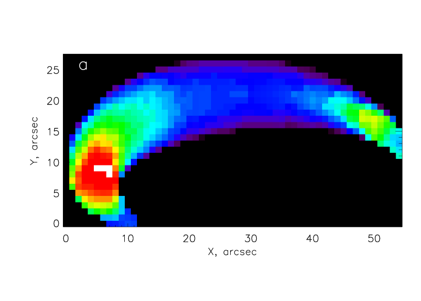
We start from a simple model of a flaring loop, which includes the following distinct elements (our model is basically similar to that proposed by Simões & Costa, 2006): 1) forming a magnetic loop from a set of field lines, which eventually represents a 3D structure consisting of a grid of volume elements (voxels) each of which is characterized by the magnetic field components , , and ; all voxel sizes were taken to be about 1”; this 3D structure is then ”observed” at an arbitrary viewing angle; 2) populating the loop by thermal plasma, i.e., prescribing the electron number density and temperature to each voxel; in general, the density and temperature can evolve in time and have an arbitrary distribution in space, but we adopted a uniform distribution of the thermal plasma for our test modeling; 3) populating the loop by fast accelerated electrons, we adopted an isotropic and spatially uniform distribution with a power-law energy spectrum; 4) calculating the gyrosynchrotron (GS) radio emission from each voxel, using the computationally fast Petrosian-Klein approximation (Petrosian, 1981; Klein, 1987) to compute the gyrosynchrotron spectrum; 5) solving the radiation transfer equation along all selected lines of sight through the rotated structure, to form the data cube of spatially resolved radio spectra for the preselected viewing angle:
| (1) |
where is the emission frequency, and are the GS emission and absorption coefficients in the Petrosian-Klein approximation (Klein, 1987) at position along the -th line of sight, is the pixel number, is the optical depth of the length of the line of sight , , and is the total length of the source along the line of sight .
This data cube (Figure 1 shows one image and one spectrum from it) represents the input information (observable in principle by an idealized radioheliograph) from which the magnetic field and other relevant flare parameters are to be determined.
3 Forward Fitting Approach
True inversion of the observational data is difficult to perform in most cases of practical importance. However, forward fitting methods can provide a good approximation to the exact solution of the problem. In this letter we concentrate on the forward fitting of the observable, spatially resolved spectra with a model spectrum with an appropriate number of free parameters, and determine the values of those free parameters based on the minimization of residuals. We point out that unlike empirical fitting methods, which use some simplified function with free parameters based on observed spectral shape (e.g., Stahli et al., 1989), and lacking a direct physical meaning, we apply the physically motivated GS source function. Although the GS source function is cumbersome in both the general case (Ramaty, 1969; Fleishman & Melnikov, 2003) and even when simplifying approximations are used (Petrosian, 1981; Klein, 1987), this approach has the great advantage that the free parameters of this fitting function are directly meaningful physical parameters.
Although each spatially resolved spectrum is originally determined from the line of sight integration (1), and so takes into account the source non-uniformity along the line of sight, the model spectrum for the forward fit is taken to be the spectrum of a homogeneous source:
| (2) |
whose parameters are to be determined from the fit.
In fact, this choice (2) is necessary because we lack reliable a priori information to include such line of sight non-uniformity. However, we expect that for many lines of sight the approximation of a uniform source is appropriate for an isolated flaring loop, allowing reliable inversion of the flare parameters (which can be checked by comparing the results with the model). Since for this first step we restrict the model to an isotropic distribution of fast electrons, we can confidently use the simplified Petrosian-Klein approximation of the gyrosynchrotron source function (Petrosian, 1981; Klein, 1987). More complicated pitch-angle distributions can in principle be used at the cost of more time-consuming calculation of the radio emission using the full expressions.
Our forward fitting scheme utilizes the downhill simplex minimization algorithm (Press et al., 1986) and so is similar to those we applied earlier (Bastian et al., 2007; Altyntsev et al., 2008; Qiu et al., 2009) but it has a few important modifications. The necessity of these modifications is called by a more complete radio spectrum from each pixel for our idealized radioheliograph, which allows the use of a source function with a larger number of free parameters than were possible in the earlier studies. In fact, we use source functions with six to eight free parameters, allowing a complete treatment of the spectrum given the types of nonthermal electron energy distributions we assume, and apply the downhill simplex minimization algorithm, which finds a local minimum of the normalized residual (or reduced chi-square). The ultimate goal of the fitting, however, is to identify the global minimum. Typically, the number of the (false) local minima increases with the number of free parameters. As has been stated, the number of the free parameters is large in our case, so the issue of the false local minima can be severe. Thus, additional measures must be taken to approach and find the true global minimum (or, at least, a nearby local minimum).
To do so, we shake the simplex solution (D.G.Yakovlev, private communication 1992) as follows (see on-line animation of the fit). The original simplex algorithms uses an -dimensional vector whose value decreases from step to step in the parametric -space leading to a local minimum of the normalized residual. When the local minimum is achieved, we strongly perturb the value of the vector and repeat the simplex minimization scheme. As a result, the system can arrive either at the same or another minimum. If it arrives at the same minimum, we treat it as the global minimum and stop the fitting of the elementary spectrum. If it arrives at a different minimum, then we select the one with the smaller residual and repeat the shaking. The new result is compared with the best one achieved so far. The number of shakings, , is limited typically to the value +6, where is the number of the free parameters. To add more flexibility to the explored parameter space we apply stronger shaking at : in addition to the increase of the vector value, we strongly change one of the free parameters. Eventually, we select the solution with the smallest normalized residual.
4 Forward Fitting Results
To perform the fitting, we must specify the source function and corresponding free parameters. As has been explained, we fit each spatially resolved spectrum (from each line of sight) with the GS solution for the homogeneous source. Since we specify the pixel size, we know the source area and the corresponding solid angle of each pixel. Thus, the free parameters are the magnetic field value () and the viewing angle () relative to the line of sight, number density of the thermal electrons (), and the parameters describing the fast electron distribution over energy. Generally, we do not know the functional shape of this distribution from first principles, thus, we use several model functions to approximate the true one. Here we start from a single power-law distribution over kinetic energy, which has three free parameters: , the number density of fast (relativistic) electrons at the kinetic energy above some threshold value (we take 100 keV as the low-energy threshold, since electrons of lower energy do not contribute substantially to the radio emission), , the energy spectral index, and , the largest energy in the electron spectrum. In terms of fitting, we use the column density, , where is the source effective depth, in place of the density , because it is that enters the GS expressions.
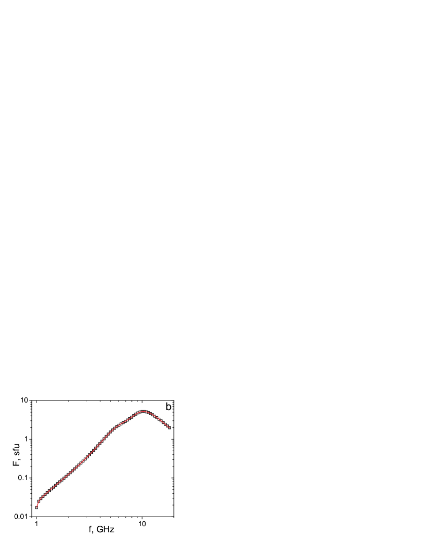
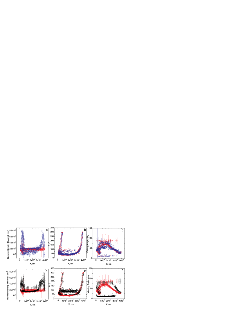
Since our model source is well resolved and consists of a few hundred line-of-sight pixels, the fitting yields corresponding 2D arrays of each of the involved free parameters. Figure 2 displays the collapsed arrays as a function of the -coordinate along the loop. Different points at each value correspond to the range of values of the individual pixels.
Let us analyze the fitting results for the assumed single power-law distribution over energy. First of all, the accuracy of the derived thermal electron number density is remarkably good: for most of the pixels the recovered values are consistent with the assumed uniform distribution with . Likewise, the plot for the recovered magnetic field values consists of a smoothly varying track, where the model magnetic field is well measured (we confirm this statement later by the direct comparison of the recovered and modeled values), although there are a number of outliers above (circled region) and below (a few points) the main track. The outliers are a consequence of finding false (local) minima of the minimized residual function. However, the outliers are a minor constituent that can easily be recognized against the true values. First, they appear at random positions in the source image and do not form a spatially coherent region, unlike the main track. Second, these same outliers are also outliers in fitted viewing angle: the bottom circled region in panel implies quasilongitudinal viewing angles, although the loop image itself (Fig. 1a) implies that the viewing angles should be quasitransverse along the loop top. Another group of outliers in viewing angle (the top circled region in panel ) has a less obvious effect on the recovered magnetic field values.
Recovery of the electron distribution parameters is also done remarkably well. The scatter in column density is related to the variation of the source depth along different pixels, while the scatter of the value is related to the fact that the GS spectrum (in the 1-18 GHz range) is almost independent of the exact value so long as it exceeds a few MeV. In contrast to , the spectral index value is recovered almost precisely, , in remarkable agreement with the model-adopted value . A few outliers (circled region) correspond to the same magnetic field value outliers circled in panel .
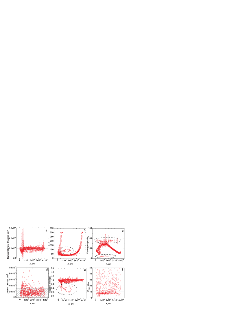
In fact, the lack of a priori knowledge on the electron distribution is one of the main potential sources of error in the recovered magnetic field. To investigate the possible range of the errors related to an incorrect choice of distribution function, we consider two plausible alternative electron distributions: (1) a double power-law (DPL) over kinetic energy, which requires two additional free parameters, the break energy and the high-energy spectral index, and (2) a single power-law distribution over the momentum modulus (PLP), which has the same number of free parameters, with the same meaning, as the single power-law distribution over energy (PLE). The overall goodness of these three fits can be evaluated based on comparison of the normalized residuals for them, Figure 3. One can see that the PLE distribution produces much smaller residuals than the other two distributions, while the DPL distribution is generally better than or comparable to the PLP distribution. We found that in our case the use of the DPL distribution, with its greater number of free parameters, is clearly excessive: the low-energy and high-energy spectral indices are close to each other and the break energy is not well defined by the fitting, which together means that the distribution is consistent with the PLE distribution with a single spectral index. We note also, that even though the DPL distribution must in principle provide as good a fit as the single PLE distribution does, the presence of two extra free parameters increases the number of local minima of the residual function so severely that the fitting frequently fails to find the true global minimum and stops at a nearby local minima.
Nevertheless, the use of the DPL distribution allows for reasonably accurate recovery of the magnetic field values along the loop, Figure 4b, comparable to the PLE distribution, although the viewing angle and the thermal electron density are recovered less precisely. In contrast, the magnetic field recovery with the PLP distribution, Figure 4e, is less accurate, especially along the loop top region. Again, these errors can easily be recognized based on apparently incorrect determination of the viewing angle, Figure 4f. Thus, the comparison of the normalized residuals for different electron distributions along with the use of the external knowledge (e.g., characteristic range of the viewing angle available from the high resolution source images) allows the outliers to be unambiguously distinguished from the true values.
5 Fitted and Model Parameter Comparison
In our model there are two values, the magnetic field and the viewing angle, which are varied through the loop and which we are going to compare with the model ones in more detail.
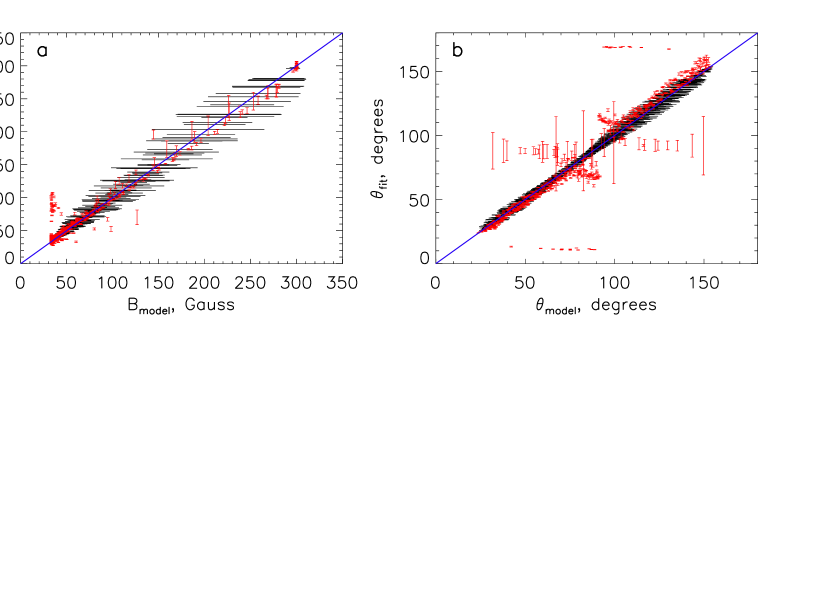
We note that both the magnetic field and the viewing angle can vary along each line of sight, while we recover single values for these parameters corresponding to a particular pixel of the source image. This means that the recovered values must be treated as effective (mean) values along each line of sight. In addition, the viewing angle values have an ambiguity between and as we use the unpolarized radio spectrum only for our fit. This ambiguity can easily be addressed by taking into account the sense of polarization observed from each pixel, which works well as is seen from Figure 5.
Figure 5 displays the direct comparison of the derived values with the model ones for the magnetic field and the viewing angle. One can clearly see that the derived magnetic field values are indeed in very close agreement with the model mean values: the formal fitting errors of the derived values are noticeably smaller than the magnetic field variation along the line of sight. Two groups of outliers seen in Figure 2 are also evident in Figure 5. The viewing angles are also recovered remarkably well (again, two groups of outliers are evident). However, the accuracy of the viewing angle recovery drops as the viewing angle approaches ; the reason for this behavior is the weak sensitivity of the GS spectrum to the exact viewing angle value when it is around . There is also a small systematic off-set of the derived values, around , compared with the mean values, whose origin is as yet unclear.
6 Discussion and Conclusions
In this Letter we have demonstrated that recovering the coronal magnetic field strength and direction via radio imaging spectroscopy data of GS emission from a flaring loop can in principle be performed with high reliability and accuracy by the appropriate forward fitting method. The potential value and application field of this finding are far-reaching. Indeed, to recover the flaring magnetic field we used a set of instantaneously measured spectra, i.e., we do not need any time integration or scanning of the loop to obtain the magnetic field along the flaring loop. Therefore, we can follow the magnetic field temporal variations, e.g., due to release of the free magnetic energy via reconnection. This offers a direct way of observing the conversion of magnetic field energy into flare energy. In addition, the simultaneous evolution of the accelerated electrons can be tracked with unprecedented accuracy through variations in their energy distribution parameters.
However, to convert the developed method to a routine, practical tool for use with future, high-resolution dynamic imaging spectroscopy data expected from the new generation of the solar radio instruments under development, we have to address a number of further issues including finite and frequency-dependent angular resolution of the instrument, statistical errors in the data, errors in the calibration, etc. In addition, we must allow at least one additional degree of freedom of the system—the possibility of anisotropic angular distributions of the fast electrons. In principle, it is easy to include the anisotropy in our method (c.f., Altyntsev et al., 2008), but this complication would greatly increase the computation time needed to obtain the solution, which calls for the development of new, computationally effective schemes of the GS calculations taking into account the anisotropy. It is worth noting that the stability of the fit can be significantly improved by using dual-polarization measurements of the spatially resolved GS spectra (Bastian, 2006), which we have not considered here.
References
- Altyntsev et al. (2008) Altyntsev, A. T., Fleishman, G. D., Huang, G.-L., & Melnikov, V. F. 2008, ApJ, 677, 1367
- Bastian (2006) Bastian, T. S. 2006, Solar Polarization 4 ASP Conference Series, R. Casini and B. W. Lites—Eds., 358,, 173
- Bastian et al. (2007) Bastian, T. S., Fleishman, G. D., & Gary, D. E. 2007, ApJ, 666, 1256
- Fleishman & Melnikov (2003) Fleishman, G. D. & Melnikov, V. F. 2003, ApJ, 587, 823
- Gary (2003) Gary, D. E. 2003, Journal of Korean Astronomical Society, 36, 135
- Gary & Hurford (1994) Gary, D. E. & Hurford, G. J. 1994, ApJ, 420, 903
- Grebinskij et al. (2000) Grebinskij, A., Bogod, V., Gelfreikh, G., Urpo, S., Pohjolainen, S., & Shibasaki, K. 2000, A&AS, 144, 169
- Kaltman et al. (2008) Kaltman, T. I., Bogod, V. M., & Yasnov, L. V. 2008, 12th European Solar Physics Meeting, Freiburg, Germany, held September, 8-12, 2008. Online at http://espm.kis.uni-freiburg.de/, p.2.89, 12, 2
- Klein (1987) Klein, K.-L. 1987, A&A, 183, 341
- Kontar et al. (2008) Kontar, E. P., Hannah, I. G., & MacKinnon, A. L. 2008, A&A, 489, L57
- Lin et al. (2004) Lin, H., Kuhn, J. R., & Coulter, R. 2004, ApJ, 613, L177
- Petrosian (1981) Petrosian, V. 1981, ApJ, 251, 727
- Press et al. (1986) Press, W. H., Flannery, B. P., & Teukolsky, S. A. 1986, Numerical recipes. The art of scientific computing (Cambridge: University Press, 1986)
- Qiu et al. (2009) Qiu, J., Gary, D. E., & Fleishman, G. D. 2009, Sol. Phys., 255, 107
- Ramaty (1969) Ramaty, R. 1969, ApJ, 158, 753
- Ryabov et al. (1999) Ryabov, B. I., Pilyeva, N. A., Alissandrakis, C. E., Shibasaki, K., Bogod, V. M., Garaimov, V. I., & Gelfreikh, G. B. 1999, Sol. Phys., 185, 157
- Simões & Costa (2006) Simões, P. J. A. & Costa, J. E. R. 2006, A&A, 453, 729
- Stahli et al. (1989) Stahli, M., Gary, D. E., & Hurford, G. J. 1989, Sol. Phys., 120, 351
- Wang (2006) Wang, H. 2006, ApJ, 649, 490