Recent Results
on the Periodic Lorentz Gas

Abstract.

The Drude-Lorentz model for the motion of electrons in a solid is a classical model in statistical mechanics, where electrons are represented as point particles bouncing on a fixed system of obstacles (the atoms in the solid). Under some appropriate scaling assumption — known as the Boltzmann-Grad scaling by analogy with the kinetic theory of rarefied gases — this system can be described in some limit by a linear Boltzmann equation, assuming that the configuration of obstacles is random [G. Gallavotti, [Phys. Rev. (2) 185 (1969), 308]). The case of a periodic configuration of obstacles (like atoms in a crystal) leads to a completely different limiting dynamics. These lecture notes review several results on this problem obtained in the past decade as joint work with J. Bourgain, E. Caglioti and B. Wennberg.

Introduction: from particle dynamics to kinetic models

The kinetic theory of gases was proposed by J. Clerk Maxwell [34, 35] and L. Boltzmann [5] in the second half of the XIXth century. Because the existence of atoms, on which kinetic theory rested, remained controversial for some time, it was not until many years later, in the XXth century, that the tools of kinetic theory became of common use in various branches of physics such as neutron transport, radiative transfer, plasma and semiconductor physics…

Besides, the arguments which Maxwell and Boltzmann used in writing what is now known as the “Boltzmann collision integral” were far from rigorous — at least from the mathematical viewpoint. As a matter of fact, the Boltzmann equation itself was studied by some of the most distinguished mathematicians of the XXth century — such as Hilbert and Carleman — before there were any serious attempt at deriving this equation from first principles (i.e. molecular dynamics.) Whether the Boltzmann equation itself was viewed as a fundamental equation of gas dynamics, or as some approximate equation valid in some well identified limit is not very clear in the first works on the subject — including Maxwell’s and Boltzmann’s.

It seems that the first systematic discussion of the validity of the Boltzmann equation viewed as some limit of molecular dynamics — i.e. the free motion of a large number of small balls subject to binary, short range interaction, for instance elastic collisions — goes back to the work of H. Grad [26]. In 1975, O.E. Lanford gave the first rigorous derivation [29] of the Boltzmann equation from molecular dynamics — his result proved the validity of the Boltzmann equation for a very short time of the order of a fraction of the reciprocal collision frequency. (One should also mention an earlier, “formal derivation” by C. Cercignani [12] of the Boltzmann equation for a hard sphere gas, which considerably clarified the mathematical formulation of the problem.) Shortly after Lanford’s derivation of the Boltzmann equation, R. Illner and M. Pulvirenti managed to extend the validity of his result for all positive times, for initial data corresponding with a very rarefied cloud of gas molecules [27].

An important assumption made in Boltzmann’s attempt at justifying the equation bearing his name is the “Stosszahlansatz”, to the effect that particle pairs just about to collide are uncorrelated. Lanford’s argument indirectly established the validity of Boltzmann’s assumption, at least on very short time intervals.

In applications of kinetic theory other than rarefied gas dynamics, one may face the situation where the analogue of the Boltzmann equation for monatomic gases is linear, instead of quadratic. The linear Boltzmann equation is encountered for instance in neutron transport, or in some models in radiative transfer. It usually describes a situation where particles interact with some background medium — such as neutrons with the atoms of some fissile material, or photons subject to scattering processes (Rayleigh or Thomson scattering) in a gas or a plasma.

In some situations leading to a linear Boltzmann equation, one has to think of two families of particles: the moving particles whose phase space density satisfies the linear Boltzmann equation, and the background medium that can be viewed as a family of fixed particles of a different type. For instance, one can think of the moving particles as being light particles, whereas the fixed particles can be viewed as infinitely heavier, and therefore unaffected by elastic collisions with the light particles. Before Lanford’s fundamental paper, an important — unfortunately unpublished — preprint by G. Gallavotti [19] provided a rigorous derivation of the linear Boltzmann equation assuming that the background medium consists of fixed, independent like hard spheres whose centers are distributed in the Euclidian space under Poisson’s law. Gallavotti’s argument already possessed some of the most remarkable features in Lanford’s proof, and therefore must be regarded as an essential step in the understanding of kinetic theory.

However, Boltzmann’s Stosszahlansatz becomes questionable in this kind of situation involving light and heavy particles, as potential correlations among heavy particles may influence the light particle dynamics. Gallavotti’s assumption of a background medium consisting of independent hard spheres excluded this this possibility. Yet, strongly correlated background media are equally natural, and should also be considered.

The periodic Lorentz gas discussed in these notes is one example of this type of situation. Assuming that heavy particles are located at the vertices of some lattice in the Euclidian space clearly introduces about the maximum amount of correlation between these heavy particles. This periodicity assumption entails a dramatic change in the structure of the equation that one obtains under the same scaling limit that would otherwise lead to a linear Boltzmann equation.

Therefore, studying the periodic Lorentz gas can be viewed as one way of testing the limits of the classical concepts of the kinetic theory of gases.

Acknowledgements.

Most of the material presented in these lectures is the result of collaboration with several authors: J. Bourgain, E. Caglioti, H.S. Dumas, L. Dumas and B. Wennberg, whom I wish to thank for sharing my interest for this problem. I am also grateful to C. Boldighrini and G. Gallavotti for illuminating discussions on this subject.

1. The Lorentz kinetic theory for electrons

In the early 1900’s, P. Drude [16] and H. Lorentz [30] independently proposed to describe the motion of electrons in metals by the methods of kinetic theory. One should keep in mind that the kinetic theory of gases was by then a relatively new subject: the Boltzmann equation for monatomic gases appeared for the first time in the papers of J. Clerk Maxwell [35] and L. Boltzmann [5]. Likewise, the existence of electrons had been established shortly before, in 1897 by J.J. Thomson.

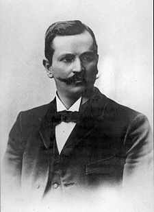
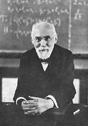
Figure 1. Left: Paul Drude (1863-1906); right: Hendrik Antoon Lorentz (1853-1928)

The basic assumptions made by H. Lorentz in his paper [30] can be summarized as follows.

First, the population of electrons is thought of as a gas of point particles described by its phase-space density $f\equiv f(t,x,v)$, that is the density of electrons at the position $x$ with velocity $v$ at time $t$.

Electron-electron collisions are neglected in the physical regime considered in the Lorentz kinetic model — on the contrary, in the classical kinetic theory of gases, collisions between molecules are important as they account for momentum and heat transfer.

However, the Lorentz kinetic theory takes into account collisions between electrons and the surrounding metallic atoms. These collisions are viewed as simple, elastic hard sphere collisions.

Since electron-electron collisions are neglected in the Lorentz model, the equation governing the electron phase-space density $f$ is linear. This is at variance with the classical Boltzmann equation, which is quadratic because only binary collisions involving pairs of molecules are considered in the kinetic theory of gases.

With the simple assumptions above, H. Lorentz arrived at the following equation for the phase-space density of electrons $f\equiv f(t,x,v)$:

$$({\partial}_{t}+v\cdot{\nabla}_{x}+\tfrac{1}{m}F(t,x)\cdot{\nabla}_{v})f(t,x,v)=N_{at}r_{at}^{2}|v|\mathcal{C}(f)(t,x,v)\,.$$

In this equation, $\mathcal{C}$ is the Lorentz collision integral, which acts on the only variable $v$ in the phase-space density $f$. In other words, for each continuous function $\phi\equiv\phi(v)$, one has

$$\mathcal{C}(\phi)(v)=\int_{|{\omega}|=1\atop{\omega}\cdot v>0}\bigl{(}\phi(v-2(v\cdot{\omega}){\omega})-\phi(v)\bigr{)}\cos(v,{\omega})d{\omega}\,,$$

and the notation

$$\mathcal{C}(f)(t,x,v)\hbox{ designates }\mathcal{C}(f(t,x,\cdot))(v)\,.$$

The other parameters involved in the Lorentz equation are the mass $m$ of the electron, and $N_{at}$, $r_{at}$ respectively the density and radius of metallic atoms. The vector field $F\equiv F(t,x)$ is the electric force. In the Lorentz model, the self-consistent electric force — i.e. the electric force created by the electrons themselves — is neglected, so that $F$ take into account the only effect of an applied electric field (if any). Roughly speaking, the self consistent electric field is linear in $f$, so that its contribution to the term $F\cdot{\nabla}_{v}f$ would be quadratic in $f$, as would be any collision integral accounting for electron-electron collisions. Therefore, neglecting electron-electron collisions and the self-consistent electric field are both in accordance with assuming that $f\ll 1$.

The line of reasoning used by H. Lorentz to arrive at the kinetic equations above is based on the postulate that the motion of electrons in a metal can be adequately represented by a simple mechanical model — a collisionless gas of point particles bouncing on a system of fixed, large spherical obstacles that represent the metallic atoms. Even with the considerable simplification in this model, the argument sketched in the article [30] is little more than a formal analogy with Boltzmann’s derivation of the equation now bearing his name.

This suggests the mathematical problem, of deriving the Lorentz kinetic equation from a microscopic, purely mechanical particle model. Thus, we consider a gas of point particles (the electrons) moving in a system of fixed spherical obstacles (the metallic atoms). We assume that collisions between the electrons and the metallic atoms are perfectly elastic, so that, upon colliding with an obstacle, each point particle is specularly reflected on the surface of that obstacle.

Undoubtedly, the most interesting part of the Lorentz kinetic equation is the collision integral which does not seem to involve $F$. Therefore we henceforth assume for the sake of simplicity that there is no applied electric field, so that

$$F(t,x)\equiv 0\,.$$

In that case, electrons are not accelerated between successive collisions with the metallic atoms, so that the microscopic model to be considered is a simple, dispersing billiard system — also called a Sinai billiard. In that model, electrons are point particles moving at a constant speed along rectilinear trajectories in a system of fixed spherical obstacles, and specularly reflected at the surface of the obstacles.

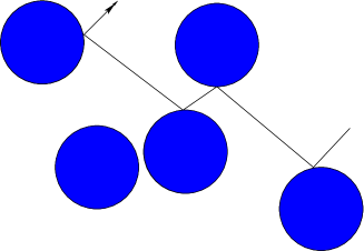
Figure 2. The Lorentz gas: a particle path

More than 100 years have elapsed since this simple mechanical model was proposed by P. Drude and H. Lorentz, and today we know that the motion of electrons in a metal is a much more complicated physical phenomenon whose description involves quantum effects.

Yet the Lorentz gas is an important object of study in nonequilibrium satistical mechanics, and there is a very significant amount of literature on that topic — see for instance [44] and the references therein.

The first rigorous derivation of the Lorentz kinetic equation is due to G. Gallavotti [18, 19], who derived it from from a billiard system consisting of randomly (Poisson) distributed obstacles, possibly overlapping, considered in some scaling limit — the Boltzmann-Grad limit, whose definition will be given (and discussed) below. Slightly more general, random distributions of obstacles were later considered by H. Spohn in [43].

While Gallavotti’s theorem bears on the convergence of the mean electron density (averaging over obstacle configurations), C. Boldrighini, L. Bunimovich and Ya. Sinai [4] later succeeded in proving the almost sure convergence (i.e. for a.e. obstacle configuration) of the electron density to the solution of the Lorentz kinetic equation.

In any case, none of the results above says anything on the case of a periodic distribution of obstacles. As we shall see, the periodic case is of a completely different nature — and leads to a very different limiting equation, involving a phase-space different from the one considered by H. Lorentz — i.e. $\mathbf{R}^{2}\times\mathbf{S}^{1}$ — on which the Lorentz kinetic equation is posed.

The periodic Lorentz gas is at the origin of many challenging mathematical problems. For instance, in the late 1970s, L. Bunimovich and Ya. Sinai studied the periodic Lorentz gas in a scaling limit different from the Boltzmann-Grad limit studied in the present paper. In [7], they showed that the classical Brownian motion is the limiting dynamics of the Lorentz gas under that scaling assumption — their work was later extended with N. Chernov: see [8]. This result is indeed a major achievement in nonequilibrium statistical mechanics, as it provides an example of an irreversible dynamics (the heat equation associated with the classical Brownian motion) that is derived from a reversible one (the Lorentz gas dynamics).

2. The Lorentz gas in the Boltzmann-Grad limit
with a Poisson distribution of obstacles

Before discussing the Boltzmann-Grad limit of the periodic Lorentz gas, we first give a brief description of Gallavotti’s result [18, 19] for the case of a Poisson distribution of independent, and therefore possibly overlapping obstacles. As we shall see, Gallavotti’s argument is in some sense fairly elementary, and yet brilliant.

First we define the notion of a Poisson distribution of obstacles. Henceforth, for the sake of simplicity, we assume a $2$-dimensional setting.

The obstacles (metallic atoms) are disks of radius $r$ in the Euclidian plane $\mathbf{R}^{2}$, centered at $c_{1},c_{2},\ldots,c_{j},\ldots\in\mathbf{R}^{2}$. Henceforth, we denote by

$$\{c\}=\{c_{1},c_{2},\ldots,c_{j},\ldots\}=\hbox{ a configuration of obstacle centers.}$$

We further assume that the configurations of obstacle centers $\{c\}$ are distributed under Poisson’s law with parameter $n$, meaning that

$$\hbox{Prob}(\{\{c\}\,|\,\#(A\cap\{c\})=p\})=e^{-n|A|}\frac{(n|A|)^{p}}{p!}\,,$$

where $|A|$ denotes the surface, i.e. the $2$-dimensional Lebesgue measure of a measurable subset $A$ of the Euclidian plane $\mathbf{R}^{2}$.

This prescription defines a probability on countable subsets of the Euclidian plane $\mathbf{R}^{2}$.

Obstacles may overlap: in other words, configurations $\{c\}$ such that

$$\hbox{for some $j\not=k\in\{1,2,\ldots\}$, one has }|c_{i}-c_{j}|<2r$$

are not excluded. Indeed, excluding overlapping obstacles means rejecting obstacles configurations $\{c\}$ such that $|c_{i}-c_{j}|\leq 2r$ for some $i,j\in\mathbf{N}$. In other words, $\hbox{Prob}(d\{c\})$ is replaced with

$$\frac{1}{Z}\prod_{i>j\geq 0}{\bf 1}_{|c_{i}-c_{j}|>2r}\hbox{Prob}(d\{c\})\,,$$

(where $Z>0$ is a normalizing coefficient.) Since the term

$$\prod_{i>j\geq 0}{\bf 1}_{|c_{i}-c_{j}|>2r}\hbox{ is not of the form }\prod_{k\geq 0}\phi_{k}(c_{k})\,,$$

the obstacles are no longer independent under this new probability measure.

Next we define the billiard flow in a given obstacle configuration $\{c\}$. This definition is self-evident, and we give it for the sake of completeness, as well as in order to introduce the notation.

Given a countable subset $\{c\}$ of the Euclidian plane $\mathbf{R}^{2}$, the billiard flow in the system of obstacles defined by $\{c\}$ is the family of mappings

$$(X(t;\cdot,\cdot,\{c\}),V(t;\cdot,\cdot,\{c\})):\,\left(\mathbf{R}^{2}\setminus\bigcup_{j\geq 1}B(c_{j},r)\right)\times\mathbf{S}^{1}\circlearrowright$$

defined by the following prescription.

Whenever the position $X$ of a particle lies outside the surface of any obstacle, that particle moves at unit speed along a rectilinear path:

$$\dot{X}(t;x,v,\{c\}) =V(t;x,v,\{c\})\,,$$

$$\dot{V}(t;x,v,\{c\}) =0\,,\qquad\hbox{ whenever }|X(t;x,v,\{c\})-c_{i}|>r\hbox{ for all }i\,,$$

and, in case of a collision with the $i$-th obstacle, is specularly reflected on the surface of that obstacle at the point of impingement, meaning that

$$X(t+0;x,v,\{c\}) =X(t-0;x,v,\{c\})\in{\partial}B(c_{i},r)\,,$$

$$V(t+0;x,v,\{c\}) =\mathcal{R}\left[\frac{X(t;x,v,\{c\})-c_{i}}{r}\right]V(t-0;x,v,\{c\})\,,$$

where $\mathcal{R}[{\omega}]$ denotes the reflection with respect to the line $(\mathbf{R}{\omega})^{\bot}$:

$$\mathcal{R}[{\omega}]v=v-2({\omega}\cdot v){\omega}\,,\quad|{\omega}|=1\,.$$

Then, given an initial probability density $f_{\{c\}}^{in}\equiv f_{\{c\}}^{in}(x,v)$ on the single-particle phase-space with support outside the system of obstacles defined by $\{c\}$, we define its evolution under the billiard flow by the formula

$$f(t,x,v,\{c\})=f^{in}_{\{c\}}(X(-t;x,v,\{c\}),V(-t;x,v,\{c\}))\,,\quad t\geq 0\,.$$

Let $\tau_{1}(x,v,\{c\}),\tau_{2}(x,v,\{c\}),\ldots,\tau_{j}(x,v,\{c\}),\ldots$ be the sequence of collision times for a particle starting from $x$ in the direction $-v$ at $t=0$ in the configuration of obstacles $\{c\}$: in other words,

$$\tau_{j}(x,v,\{c\})=$$

$$\quad\sup\{t\,|\,\#\{s\in[0,t]\,|\,\hbox{dist}(X(-s,x,v,\{c\});\{c\})=r\}=j-1\}\,.$$

Denoting $\tau_{0}=0$ and ${\Delta}\tau_{k}=\tau_{k}-\tau_{k-1}$, the evolved single-particle density $f$ is a.e. defined by the formula

$$f(t,x,v,\{c\})=f^{in}(x-tv,v){\bf 1}_{t<\tau_{1}}$$

$$+\!\sum_{j\geq 1}\!f^{in}\!\left(x\!-\!\!\!\sum_{k=1}^{j}\!\!{\Delta}\tau_{k}V(-\tau_{k}^{-})\!-\!(t-\tau_{j})V(-\tau_{j}^{+}),V(-\tau_{j}^{+})\right)\!{\bf 1}_{\tau_{j}<t<\tau_{j+1}}\,.$$

In the case of physically admissible initial data, there should be no particle located inside an obstacle. Hence we assumed that $f^{in}_{\{c\}}=0$ in the union of all the disks of radius $r$ centered at the $c_{j}\in\{c\}$. By construction, this condition is obviously preserved by the billiard flow, so that $f(t,x,v,\{c\})$ also vanishes whenever $x$ belongs to a disk of radius $r$ centered at any $c_{j}\in\{c\}$.

As we shall see shortly, when dealing with bounded initial data, this constraint disappears in the (yet undefined) Boltzmann-Grad limit, as the volume fraction occupied by the obstacles vanishes in that limit.

Therefore, we shall henceforth neglect this difficulty and proceed as if $f^{in}$ were any bounded probability density on $\mathbf{R}^{2}\times\mathbf{S}^{1}$.

Our goal is to average the summation above in the obstacle configuration $\{c\}$ under the Poisson distribution, and to identify a scaling on the obstacle radius $r$ and the parameter $n$ of the Poisson distribution leading to a nontrivial limit.

The parameter $n$ has the following important physical interpretation. The expected number of obstacle centers to be found in any measurable subset ${\Omega}$ of the Euclidian plane $\mathbf{R}^{2}$ is

$$\sum_{p\geq 0}p\hbox{Prob}(\{\{c\}\,|\,\#({\Omega}\cap\{c\})=p\})=\sum_{p\geq 0}pe^{-n|{\Omega}|}\frac{(n|{\Omega}|)^{p}}{p!}=n|{\Omega}|$$

so that

$$n=\#\hbox{ obstacles per unit surface in $\mathbf{R}^{2}$.}$$

The average of the first term in the summation defining $f(t,x,v,\{c\})$ is

$$f^{in}(x-tv,v)\langle{\bf 1}_{t<\tau_{1}}\rangle=f^{in}(x-tv,v)e^{-n2rt}$$

(where $\langle\,\cdot\,\rangle$ denotes the mathematical expectation) since the condition $t<\tau_{1}$ means that the tube of width $2r$ and length $t$ contains no obstacle center.

Figure 3. The tube corresponding with the first term in the series expansion giving the particle density

Henceforth, we seek a scaling limit corresponding to small obstacles, i.e. $r\to 0$ and a large number of obstacles per unit volume, i.e. $n\to\infty$.

There are obviously many possible scalings satisfying this requirement. Among all these scalings, the Boltzmann-Grad scaling in space dimension $2$ is defined by the requirement that the average over obstacle configurations of the first term in the series expansion for the particle density $f$ has a nontrivial limit.

Boltzmann-Grad scaling in space dimension 2

In order for the average of the first term above to have a nontrivial limit, one must have

$$r\to 0^{+}\hbox{ and }n\to+\infty\hbox{ in such a way that }2nr\to{\sigma}>0\,.$$

Under this assumption

$$\langle f^{in}(x-tv,v){\bf 1}_{t<\tau_{1}}\rangle\to f^{in}(x-tv,v)e^{-{\sigma}t}\,.$$

Gallavotti’s idea is that this first term corresponds with the solution at time $t$ of the equation

$$({\partial}_{t}+v\cdot{\nabla}_{x})f =-nrf\int_{|{\omega}|=1\atop{\omega}\cdot v>0}\cos(v,{\omega})d{\omega}=-2nrf$$

$$f{\big{|}}_{t=0} =f^{in}$$

that involves only the loss part in the Lorentz collision integral, and that the (average over obstacle configuration of the) subsequent terms in the sum defining the particle density $f$ should converge to the Duhamel formula for the Lorentz kinetic equation.

After this necessary preliminaries, we can state Gallavotti’s theorem.

Theorem 2.1 (Gallavotti [19]).

Let $f^{in}$ be a continuous, bounded probability density on $\mathbf{R}^{2}\times\mathbf{S}^{1}$, and let

$$f_{r}(t,x,v,\{c\})=f^{in}((X^{r},V^{r})(-t,x,v,\{c\}))\,,$$

where $(t,x,v)\mapsto(X^{r},V^{r})(t,x,v,\{c\})$ is the billiard flow in the system of disks of radius $r$ centered at the elements of $\{c\}$. Assuming that the obstacle centers are distributed under the Poisson law of parameter $n={\sigma}/2r$ with ${\sigma}>0$, the expected single particle density

$$\langle f_{r}(t,x,v,\cdot)\rangle\to f(t,x,v)\hbox{ in }L^{1}(\mathbf{R}^{2}\times\mathbf{S}^{1})$$

uniformly on compact $t$-sets, where $f$ is the solution of the Lorentz kinetic equation

$$({\partial}_{t}+v\cdot{\nabla}_{x})f+{\sigma}f ={\sigma}\int_{0}^{2\pi}f(t,x,R[{\beta}]v)\sin\tfrac{{\beta}}{2}\tfrac{d{\beta}}{4}\,,$$

$$f{\big{|}}_{t=0} =f^{in}\,,$$

where $R[{\beta}]$ denotes the rotation of an angle ${\beta}$.

End of the proof of Gallavotti’s theorem.

The general term in the summation giving $f(t,x,v,\{c\})$ is

$$f^{in}\!\left(x\!-\!\!\!\sum_{k=1}^{j}\!\!{\Delta}\tau_{k}V^{r}(-\tau_{k}^{-})\!-\!(t-\tau_{j})V^{r}(-\tau_{j}^{+}),V^{r}(-\tau_{j}^{+})\right)\!{\bf 1}_{\tau_{j}<t<\tau_{j+1}}\,,$$

and its average under the Poisson distribution on $\{c\}$ is

$$\int f^{in}\!\left(x-\!\sum_{k=1}^{j}{\Delta}\tau_{k}V^{r}(-\tau_{k}^{-})-(t-\tau_{j})V^{r}(-\tau_{j}^{+}),V^{r}(-\tau_{j}^{-})\right)$$

$$e^{-n|T(t;c_{1},\ldots,c_{j})|}\frac{n^{j}dc_{1}\ldots dc_{j}}{j!}\,,$$

where $T(t;c_{1},\ldots,c_{j})$ is the tube of width $2r$ around the particle trajectory colliding first with the obstacle centered at $c_{1}$, …, and whose $j$-th collision is with the obstacle centered at $c_{j}$.

As before, the surface of that tube is

$$|T(t;c_{1},\ldots,c_{j})|=2rt+O(r^{2})\,.$$

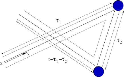
Figure 4. The tube $T(t,c_{1},c_{2})$ corresponding with the third term in the series expansion giving the particle density

In the $j$-th term, change variables by expressing the positions of the $j$ encountered obstacles in terms of free flight times and deflection angles:

$$(c_{1},\ldots,c_{j})\mapsto(\tau_{1},\ldots,\tau_{j};{\beta}_{1},\ldots,{\beta}_{j})\,.$$

The volume element in the $j$-th integral is changed into

$$\tfrac{dc_{1}\ldots dc_{j}}{j!}=r^{j}\sin\tfrac{{\beta}_{1}}{2}\ldots\sin\tfrac{{\beta}_{j}}{2}\,\,\tfrac{d{\beta}_{1}}{2}\ldots\tfrac{d{\beta}_{j}}{2}d\tau_{1}\ldots d\tau_{j}\,.$$

The measure in the left-hand side is invariant by permutations of $c_{1},\ldots,c_{j}$; on the right-hand side, we assume that

$$\tau_{1}<\tau_{2}<\ldots<\tau_{j}\,,$$

which explains why $1/j!$ factor disappears in the right-hand side.

Figure 5. The substitution $(c_{1},c_{2})\mapsto(\tau_{1},\tau_{2},{\beta}_{1},{\beta}_{2})$

The substitution above is one-to-one only if the particle does not hit twice the same obstacle. Define therefore

$$A_{r}(T,x,v)=\{\{c\}\,|\,\hbox{ there exists }0<t_{1}<t_{2}<T\hbox{ and }j\in\mathbf{N}\hbox{ s.t. }$$

$$\qquad\qquad\qquad\hbox{dist}(X^{r}(t_{1},x,v,\{c\}),c_{j})=\hbox{dist}(X^{r}(t_{2},x,v,\{c\}),c_{j})=r\}$$

$$\qquad=\bigcup_{j\geq 1}\{\{c\}\,|\,\hbox{dist}(X^{r}(t,x,v,\{c\}),c_{j})=r\hbox{ for some }0<t_{1}<t_{2}<T\}\,,$$

and set

$$f^{M}_{r}(t,x,v,\{c\}) =f_{r}(t,x,v,\{c\})-f^{R}_{r}(t,x,v,\{c\})\,,$$

$$f^{R}_{r}(t,x,v,\{c\}) =f_{r}(t,x,v,\{c\}){\bf 1}_{A_{r}(T,x,v)}(\{c\})\,,$$

respectively the Markovian part and the recollision part in $f_{r}$.

After averaging over the obstacle configuration $\{c\}$, the contribution of the $j$-th term in $f^{M}_{r}$ is, to leading order in $r$:

$$(2nr)^{j}e^{-2nrt}\int_{0<\tau_{1}<\ldots<\tau_{j}<t}\int_{[0,{2\pi}]^{j}}\sin\tfrac{{\beta}_{1}}{2}\ldots\sin\tfrac{{\beta}_{j}}{2}\tfrac{d{\beta}_{1}}{4}\ldots\tfrac{d{\beta}_{j}}{4}d\tau_{1}\ldots d\tau_{j}$$

$$\times f^{in}\left(x\!-\!\!\!\sum_{k=1}^{j}\!\!{\Delta}\tau_{k}R\left[\sum_{l=1}^{k-1}{\beta}_{l}\right]v\!-\!(t-\tau_{j})R\left[\sum_{l=1}^{j-1}{\beta}_{l}\right]v,R\left[\sum_{l=1}^{j}{\beta}_{l}\right]v\right)\,.$$

It is dominated by

$$\|f^{in}\|_{L^{\infty}}O({\sigma})^{j}e^{-O({\sigma})t}\frac{t^{j}}{j!}$$

which is the general term of a converging series.

Passing to the limit as $n\to+\infty$, $r\to 0$ so that $2rn\to{\sigma}$, one finds (by dominated convergence in the series) that

$$\langle f^{M}_{r}(t,x,v,\{c\})\rangle\to e^{-{\sigma}t}f^{in}(x-tv,v)$$

$$+{\sigma}e^{-{\sigma}t}\int_{0}^{t}\int_{0}^{2\pi}f^{in}(x-\tau_{1}v-(t-\tau_{1})R[{\beta}_{1}]v,R[{\beta}_{1}]v)\sin\tfrac{{\beta}_{1}}{2}\tfrac{d{\beta}_{1}}{4}d\tau_{1}$$

$$+\sum_{j\geq 2}{\sigma}^{j}e^{-{\sigma}t}\int_{0<\tau_{j}<\ldots<\tau_{1}<t}\int_{[0,{2\pi}]^{j}}\sin\tfrac{{\beta}_{1}}{2}\ldots\sin\tfrac{{\beta}_{j}}{2}$$

$$\times f^{in}\left(x\!-\!\!\!\sum_{k=1}^{j}\!\!{\Delta}\tau_{k}R\left[\sum_{l=1}^{k-1}{\beta}_{l}\right]v\!-\!(t-\tau_{j})R\left[\sum_{l=1}^{j-1}{\beta}_{l}\right]v,R\left[\sum_{l=1}^{j}{\beta}_{l}\right]v\right)$$

$$\times\tfrac{d{\beta}_{1}}{4}\ldots\tfrac{d{\beta}_{j}}{4}d\tau_{1}\ldots d\tau_{j}\,,$$

which is the Duhamel series giving the solution of the Lorentz kinetic equation.

Hence, we have proved that

$$\langle f^{M}_{r}(t,x,v,\cdot)\rangle\to f(t,x,v)\hbox{ uniformly on bounded sets as }r\to 0^{+}\,,$$

where $f$ is the solution of the Lorentz kinetic equation. One can check by a straightforward computation that the Lorentz collision integral satisfies the property

$$\int_{\mathbf{S}^{1}}\mathcal{C}(\phi)(v)dv=0\hbox{ for each }\phi\in L^{\infty}(\mathbf{S}^{1})\,.$$

Integrating both sides of the Lorentz kinetic equation in the variables $(t,x,v)$ over $[0,t]\times\mathbf{R}^{2}\times\mathbf{S}^{1}$ shows that the solution $f$ of that equation satisfies

$$\iint_{\mathbf{R}^{2}\times\mathbf{S}^{1}}f(t,x,v)dxdv=\iint_{\mathbf{R}^{2}\times\mathbf{S}^{1}}f^{in}(x,v)dxdv$$

for each $t>0$.

On the other hand, the billiard flow $(X,V)(t,\cdot,\cdot,\{c\})$ obviously leaves the uniform measure $dxdv$ on $\mathbf{R}^{2}\times\mathbf{S}^{1}$ (i.e. the particle number) invariant, so that, for each $t>0$ and each $r>0$,

$$\iint_{\mathbf{R}^{2}\times\mathbf{S}^{1}}f_{r}(t,x,v,\{c\})dxdv=\iint_{\mathbf{R}^{2}\times\mathbf{S}^{1}}f^{in}(x,v)dxdv\,.$$

We therefore deduce from Fatou’s lemma that

$$\langle f^{R}_{r}\rangle\to 0\hbox{ in }L^{1}(\mathbf{R}^{2}\times\mathbf{S}^{1})\hbox{ uniformly on bounded $t$-sets}$$

$$\langle f^{M}_{r}\rangle\to f\hbox{ in }L^{1}(\mathbf{R}^{2}\times\mathbf{S}^{1})\hbox{ uniformly on bounded $t$-sets}$$

which concludes our sketch of the proof of Gallavotti’s theorem. ∎

For a complete proof, we refer the interested reader to [19, 20].

Some remarks are in order before leaving Gallavotti’s setting for the Lorentz gas with the Poisson distribution of obstacles.

Assuming no external force field as done everywhere in the present paper is not as inocuous as it may seem. For instance, in the case of Poisson distributed holes — i.e. purely absorbing obstacles, so that particles falling into the holes disappear from the system forever — the presence of an external force may introduce memory effects in the Boltzmann-Grad limit, as observed by L. Desvillettes and V. Ricci [15].

Another remark is about the method of proof itself. One has obtained the Lorentz kinetic equation after having obtained an explicit formula for the solution of that equation. In other words, the equation is deduced from the solution — which is a somewhat unusual situation in mathematics. However, the same is true of Lanford’s derivation of the Boltzmann equation [29], as well as of the derivation of several other models in nonequilibrium statistical mechanics. For an interesting comment on this issue, see [13], on p. 75.

3. Santaló’s formula
for the geometric mean free path

From now on, we shall abandon the random case and concentrate our efforts on the periodic Lorentz gas.

Our first task is to define the Boltzmann-Grad scaling for periodic systems of spherical obstacles. In the Poisson case defined above, things were relatively easy: in space dimension $2$, the Boltzmann-Grad scaling was defined by the prescription that the number of obstacles per unit volume tends to infinity while the obstacle radius tends to $0$ in such a way that

$$\#\hbox{ obstacles per unit volume }\times\hbox{ obstacle radius }\to{\sigma}>0\,.$$

The product above has an interesting geometric meaning even without assuming a Poisson distribution for the obstacle centers, which we shall briefly discuss before going further in our analysis of the periodic Lorentz gas.

Perhaps the most important scaling parameter in all kinetic models is the mean free path. This is by no means a trivial notion, as will be seen below. As suggested by the name itself, any notion of mean free path must involve first the notion of free path length, and then some appropriate probability measure under which the free path length is averaged.

For simplicity, the only periodic distribution of obstacles considered below is the set of balls of radius $r$ centered at the vertices of a unit cubic lattice in the $D$-dimensional Euclidian space.

Correspondingly, for each $r\in(0,\tfrac{1}{2})$, we define the domain left free for particle motion, also called the “billiard table” as

$$Z_{r}=\{x\in\mathbf{R}^{D}\,|\,\hbox{dist}(x,\mathbf{Z}^{D})>r\}\,.$$

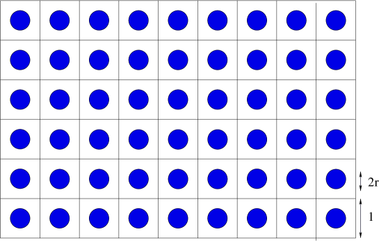
Figure 6. The periodic billiard table

Defining the free path length in the billiard table $Z_{r}$ is easy: the free path length starting from $x\in Z_{r}$ in the direction $v\in\mathbf{S}^{D-1}$ is

$$\tau_{r}(x,v)=\min\{t>0\,|\,x+tv\in{\partial}Z_{r}\}\,.$$

Obviously, for each $v\in\mathbf{S}^{D-1}$ the free path length $\tau_{r}(\cdot,v)$ in the direction $v$ can be extended continuously to

$$\{x\in{\partial}Z_{r}\,|\,v\cdot n_{x}\not=0\}\,,$$

where $n_{x}$ denotes the unit normal vector to ${\partial}Z_{r}$ at the point $x\in{\partial}Z_{r}$ pointing towards $Z_{r}$.

With this definition, the mean free path is the quantity defined as

$$\hbox{Mean Free Path}=\langle\tau_{r}\rangle\,,$$

where the notation $\langle\cdot\rangle$ designates the average under some appropriate probability measure on $\overline{Z_{r}}\times\mathbf{S}^{D-1}$.

Figure 7. The free path length

A first ambiguity in the notion of mean free path comes from the fact that there are two fairly natural probability measures for the Lorentz gas.

The first one is the uniform probability measure on $Z_{r}/\mathbf{Z}^{D}\times\mathbf{S}^{D-1}$

$$d\mu_{r}(x,v)=\frac{dxdv}{|Z_{r}/\mathbf{Z}^{D}|\,|\mathbf{S}^{D-1}|}$$

that is invariant under the billiard flow — the notation $|\mathbf{S}^{D-1}|$ designates the $D-1$-dimensional uniform measure of the unit sphere $\mathbf{S}^{D-1}$. This measure is obviously invariant under the billiard flow

$$(X_{r},V_{r})(t,\cdot,\cdot):\,Z_{r}\times\mathbf{S}^{D-1}\to Z_{r}\times\mathbf{S}^{D-1}$$

defined by

$$\left\{\begin{matrix}\dot{X}_{r}=V_{r}\\ \dot{V}_{r}=0\end{matrix}\right.\quad\hbox{ whenever }X(t)\notin{\partial}Z_{r}$$

while

$$\left\{\begin{array}[]{l}X_{r}(t^{+})=X_{r}(t^{-})=:X_{r}(t)\hbox{ if }X(t^{\pm})\in{\partial}Z_{r}\,,\\ V_{r}(t^{+})=\mathcal{R}[n_{X_{r}(t)}]V_{r}(t^{-})\end{array}\right.$$

with $\mathcal{R}[n]v=v-2v\!\cdot\!nn$ denoting the reflection with respect to the hyperplane $(\mathbf{R}n)^{\bot}$.

The second such probability measure is the invariant measure of the billiard map

$$d\nu_{r}(x,v)=\frac{v\!\cdot\!n_{x}dS(x)dv}{v\!\cdot\!n_{x}dxdv\hbox{-meas}(\Gamma^{r}_{+}/\mathbf{Z}^{D})}$$

where $n_{x}$ is the unit inward normal at $x\in{\partial}Z_{r}$, while $dS(x)$ is the $D-1$-dimensional surface element on ${\partial}Z_{r}$, and

$$\Gamma^{r}_{+}:=\{(x,v)\in{\partial}Z_{r}\times\mathbf{S}^{D-1}\,|\,v\cdot n_{x}>0\}\,.$$

The billiard map $\mathcal{B}_{r}$ is the map

$$\Gamma^{r}_{+}\ni(x,v)\mapsto\mathcal{B}_{r}(x,v):=(X_{r},V_{r})(\tau_{r}(x,v);x,v)\in\Gamma^{r}_{+}\,,$$

which obviously passes to the quotient modulo $\mathbf{Z}^{D}$-translations:

$$\mathcal{B}_{r}:\;\Gamma^{r}_{+}/\mathbf{Z}^{D}\to\Gamma^{r}_{+}/\mathbf{Z}^{D}\,.$$

In other words, given the position $x$ and the velocity $v$ of a particle immediatly after its first collision with an obstacle, the sequence $(\mathcal{B}^{n}_{r}(x,v))_{n\geq 0}$ is the sequence of all collision points and post-collision velocities on that particle’s trajectory.

With the material above, we can define a first, very natural notion of mean free path, by setting

$$\hbox{Mean Free Path}=\lim_{N\to+\infty}\frac{1}{N}\sum_{k=0}^{N-1}\tau_{r}(\mathcal{B}^{k}_{r}(x,v))\,.$$

Notice that, for $\nu_{r}$-a.e. $(x,v)\in\Gamma^{+}_{r}/\mathbf{Z}^{D}$, the right hand side of the equality above is well-defined by the Birkhoff ergodic theorem. If the billiard map $\mathcal{B}_{r}$ is ergodic for the measure $\nu_{r}$, one has

$$\lim_{N\to+\infty}\frac{1}{N}\sum_{k=0}^{N-1}\tau_{r}(\mathcal{B}^{k}_{r}(x,v))=\int_{\Gamma^{r}_{+}/{\mathbf{Z}^{D}}}\tau_{r}d\nu_{r}\,,$$

for $\nu_{r}$-a.e. $(x,v)\in\Gamma^{r}_{+}/\mathbf{Z}^{D}$.

Now, a very general formula for computing the right-hand side of the above equality was found by the great spanish mathematician L. A. Santaló in 1942. In fact, Santaló’s argument applies to situations that are considerably more general, involving for instance curved trajectories instead of straight line segments, or obstacle distributions other than periodic. The reader interested in these questions is referred to Santaló’s original article [38].

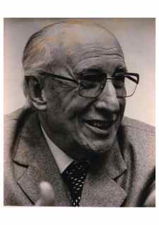
Figure 8. Luis Antonio Santaló Sors (1911-2001)

Here is

Santaló’s formula for the geometric mean free path

One finds that

$$\ell_{r}:=\int_{\Gamma^{r}_{+}/{\mathbf{Z}^{D}}}\tau_{r}(x,v)d\nu_{r}(x,v)=\frac{1-|\mathbf{B}^{D}|r^{D}}{|\mathbf{B}^{D-1}|r^{D-1}}$$

where $\mathbf{B}^{D}$ is the unit ball of $\mathbf{R}^{D}$ and $|\mathbf{B}^{D}|$ its $D$-dimensional Lebesgue measure.

In fact, one has the following slightly more general

Lemma 3.1 (H.S. Dumas, L. Dumas, F. Golse [17]).

For $f\in C^{1}(\mathbf{R}_{+})$ such that $f(0)=0$, one has

$$\iint_{\Gamma^{r}_{+}/\mathbf{Z}^{D}}f(\tau_{r}(x,v))v\cdot n_{x}dS(x)dv=\iint_{(Z_{r}/\mathbf{Z}^{D})\times\mathbf{S}^{D-1}}f^{\prime}(\tau_{r}(x,v))dxdv\,.$$

Santaló’s formula is obtained by setting $f(z)=z$ in the identity above, and expressing both integrals in terms of the normalized measures $\nu_{r}$ and $\mu_{r}$.

Proof.

For each $(x,v)\in Z_{r}\times\mathbf{S}^{D-1}$ one has

$$\tau_{r}(x+tv,v)=\tau_{r}(x,v)-t\,,$$

so that

$$\frac{d}{dt}\tau_{r}(x+tv,v)=-1\,.$$

Hence $\tau_{r}(x,v)$ solves the transport equation

$$\left\{\begin{array}[]{lll}v\cdot{\nabla}_{x}\tau_{r}(x,v)=-1\,,&\quad x\in Z_{r}\,,&v\in\mathbf{S}^{D-1}\,,\\ \tau_{r}(x,v)=0\,,&\quad x\in{\partial}Z_{r}\,,&v\cdot n_{x}<0\,.\end{array}\right.$$

Since $f\in C^{1}(\mathbf{R}_{+})$ and $f(0)=0$, one has

$$\left\{\begin{array}[]{lll}v\cdot{\nabla}_{x}f(\tau_{r}(x,v))=-f^{\prime}(\tau_{r}(x,v))\,,&\quad x\in Z_{r}\,,&v\in\mathbf{S}^{D-1}\,,\\ f(\tau_{r}(x,v))=0\,,&\quad x\in{\partial}Z_{r}\,,&v\cdot n_{x}<0\,.\end{array}\right.$$

Integrating both sides of the equality above, and applying Green’s formula shows that

$$-\iint_{(Z_{r}/\mathbf{Z}^{D})\times\mathbf{S}^{D-1}} f^{\prime}(\tau_{r}(x,v))dxdv$$

$$=\iint_{(Z_{r}/\mathbf{Z}^{D})\times\mathbf{S}^{D-1}}v\cdot{\nabla}_{x}(f(\tau_{r}(x,v)))dxdv$$

$$=-\iint_{({\partial}Z_{r}/\mathbf{Z}^{D})\times\mathbf{S}^{D-1}}f(\tau_{r}(x,v))v\cdot n_{x}dS(x)dv$$

— beware the unusual sign in the right-hand side of the second equality above, coming from the orientation of the unit normal $n_{x}$, which is pointing towards $Z_{r}$. ∎

With the help of Santaló’s formula, we define the Boltzmann-Grad limit for the Lorentz gas with periodic as well as random distribution of obstacles as follows:

Boltzmann-Grad scaling

The Boltzmann-Grad scaling for the periodic Lorentz gas in space dimension $D$ corresponds with the following choice of parameters:

distance between neighboring lattice points $$={\varepsilon}\ll 1\,,$$

obstacle radius $$=r\ll 1\,,$$

mean free path $$=\ell_{r}\to\frac{1}{{\sigma}}>0\,.$$

Santaló’s formula indicates that one should have

$$r\sim c{\varepsilon}^{\frac{D}{D-1}}\hbox{ with }c=\left(\frac{{\sigma}}{|\mathbf{B}^{D-1}|}\right)^{-\frac{1}{D-1}}\hbox{ as }{\varepsilon}\to 0^{+}\,.$$

Therefore, given an initial particle density $f^{in}\in C_{c}(\mathbf{R}^{D}\times\mathbf{S}^{D-1})$, we define $f_{r}$ to be

$$f_{r}(t,x,v)=f^{in}\left(r^{D-1}X_{r}\left(-\frac{t}{r^{D-1}};\frac{x}{r^{D-1}},v\right),V_{r}\left(-\frac{t}{r^{D-1}};\frac{x}{r^{D-1}},v\right)\right)$$

where $(X_{r},V_{r})$ is the billiard flow in $Z_{r}$ with specular reflection on ${\partial}Z_{r}$.

Notice that this formula defines $f_{r}$ for $x\in Z_{r}$ only, as the particle density should remain $0$ for all time in the spatial domain occupied by the obstacles. As explained in the previous section, this is a set whose measure vanishes in the Boltzmann-Grad limit, and we shall always implicitly extend the function $f_{r}$ defined above by $0$ for $x\notin Z_{r}$.

Since $f^{in}$ is a bounded function on $Z_{r}\times\mathbf{S}^{D-1}$, the family $f_{r}$ defined above is a bounded family of $L^{\infty}(\mathbf{R}^{D}\times\mathbf{S}^{D-1})$. By the Banach-Alaoglu theorem, this family is therefore relatively compact for the weak-* topology of $L^{\infty}(\mathbf{R}_{+}\times\mathbf{R}^{D}\times\mathbf{S}^{D-1})$.

Problem: to find an equation governing the $L^{\infty}$ weak-* limit points of the scaled number density $f_{r}$ as $r\to 0^{+}$.

In the sequel, we shall describe the answer to this question in the $2$-dimensional case ($D=2$.)

4. Estimates for the distribution of free-path lengths

In the proof of Gallavotti’s theorem for the case of a Poisson distribution of obstacles in space dimension $D=2$, the probability that a strip of width $2r$ and length $t$ does not meet any obstacle is $e^{-2nrt}$, where $n$ is the parameter of the Poisson distribution — i.e. the average number of obstacles per unit surface.

This accounts for the loss term

$$f^{in}(x-tv,v)e^{-{\sigma}t}$$

in the Duhamel series for the solution of the Lorentz kinetic equation, or of the term $-{\sigma}f$ on the right-hand side of that equation written in the form

$$({\partial}_{t}+v\cdot{\nabla}_{x})f=-{\sigma}f+{\sigma}\int_{0}^{2\pi}f(t,x,R({\beta})v)\sin\tfrac{{\beta}}{2}\tfrac{d{\beta}}{4}\,.$$

Things are fundamentally different in the periodic case. To begin with, there are infinite strips included in the billiard table $Z_{r}$ which never meet any obstacle.

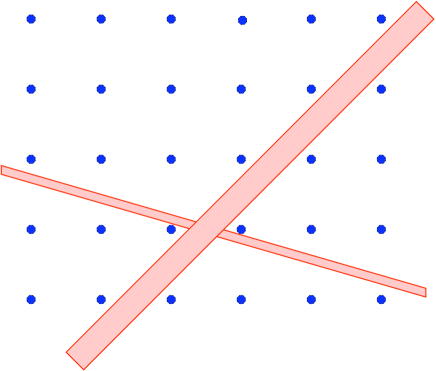
Figure 9. Open strips in the periodic billiard table that never meet any obstacle

The contribution of the 1-particle density leading to the loss term in the Lorentz kinetic equation is, in the notation of the proof of Gallavotti’s theorem

$$f^{in}(x-tv,v){\bf 1}_{t<\tau_{1}(x,v,\{c\})}\,.$$

The analogous term in the periodic case is

$$f^{in}(x-tv,v){\bf 1}_{t<r^{D-1}\tau_{r}(x/r,-v)}$$

where $\tau_{r}(x,v)$ is the free-path length in the periodic billiard table $Z_{r}$ starting from $x\in Z_{r}$ in the direction $v\in\mathbf{S}^{1}$.

Passing to the $L^{\infty}$ weak-* limit as $r\to 0$ reduces to finding

$$\lim_{r\to 0}{\bf 1}_{t<r^{D-1}\tau_{r}(x/r,-v)}\hbox{ in }w^{*}-L^{\infty}(\mathbf{R}^{2}\times\mathbf{S}^{1})\,$$

— possibly after extracting a subsequence $r_{n}\downarrow 0$. As we shall see below, this involves the distribution of $\tau_{r}$ under the probability measure $\mu_{r}$ introduced in the discussion of Santaló’s formula — i.e. assuming the initial position $x$ and direction $v$ to be independent and uniformly distributed on $(\mathbf{R}^{D}/\mathbf{Z}^{D})\times\mathbf{S}^{D-1}$.

We define the (scaled) distribution under $\mu_{r}$ of free path lengths $\tau_{r}$ to be

$$\Phi_{r}(t):=\mu_{r}(\{(x,v)\in(Z_{r}/\mathbf{Z}^{D})\times\mathbf{S}^{D-1}\,|\,\tau_{r}(x,v)>t/r^{D-1}\})\,.$$

Notice the scaling $t\mapsto t/r^{D-1}$ in this definition. In space dimension $D$, Santaló’s formula shows that

$$\iint_{\Gamma_{r}^{+}/\mathbf{Z}^{D}}\tau_{r}(x,v)d\nu_{r}(x,v)\sim\tfrac{1}{|\mathbf{B}^{D-1}|}r^{1-D}\,,$$

and this suggests that the free path length $\tau_{r}$ is a quantity of the order of $1/r^{D-1}$. (In fact, this argument is not entirely convincing, as we shall see below.)

In any case, with this definition of the distribution of free path lengths under $\mu_{r}$, one arrives at the following estimate.

Theorem 4.1 (Bourgain-Golse-Wennberg [6, 25]).

In space dimension $D\geq 2$, there exists $0<C_{D}<C^{\prime}_{D}$ such that

$$\frac{C_{D}}{t}\leq\Phi_{r}(t)\leq\frac{C^{\prime}_{D}}{t}\quad\hbox{ whenever }t>1\hbox{ and }\,0<r<\tfrac{1}{2}\,.$$

The lower bound and the upper bound in this theorem are obtained by very different means.

The upper bound follows from a Fourier series argument which is reminiscent of Siegel’s prood of the classical Minkowski convex body theorem (see [39, 36].)

The lower bound, on the other hand, is obtained by working in physical space. Specifically, one uses a channel technique, introduced independently by P. Bleher [2] for the diffusive scaling.

This lower bound alone has an important consequence:

Corollary 4.2.

For each $r>0$, the average of the free path length (mean free path) under the probability measure $\mu_{r}$ is infinite:

$$\int_{(Z_{r}/\mathbf{Z}^{D})\times\mathbf{S}^{D-1}}\tau_{r}(x,v)d\mu_{r}(x,v)=+\infty\,.$$

Proof.

Indeed, since $\Phi_{r}$ is the distribution of $\tau_{r}$ under $\mu_{r}$, one has

$$\int_{(Z_{r}/\mathbf{Z}^{D})\times\mathbf{S}^{D-1}}\tau_{r}(x,v)d\mu_{r}(x,v)=\int_{0}^{\infty}\Phi_{r}(t)dt\geq\int_{1}^{\infty}\frac{C_{D}}{t}dt=+\infty\,.$$

∎

Recall that the average of the free path length unded the “other” natural probability measure $\nu_{r}$ is precisely Santaló’s formula for the mean free path:

$$\ell_{r}=\iint_{\Gamma^{+}_{r}/\mathbf{Z}^{D}}\tau_{r}(x,v)d\nu_{r}(x,v)=\frac{1-|\mathbf{B}^{D}|r^{D}}{|\mathbf{B}^{D-1}|r^{D-1}}\,.$$

One might wonder why averaging the free path length $\tau_{r}$ under the measures $\nu_{r}$ and $\mu_{r}$ actually gives two so different results.

First observe that Santaló’s formula gives the mean free path under the probability measure $\nu_{r}$ concentrated on the surface of the obstacles, and is therefore irrelevant for particles that have not yet encountered an obstacle.

Besides, by using the lemma that implies Santaló’s formula with $f(z)=\tfrac{1}{2}z^{2}$, one has

$$\iint_{(Z_{r}/\mathbf{Z}^{D})\times\mathbf{S}^{D-1}}\tau_{r}(x,v)d\mu_{r}(x,v)=\frac{1}{\ell_{r}}\int_{\Gamma^{+}_{r}/\mathbf{Z}^{D}}\tfrac{1}{2}\tau_{r}(x,v)^{2}d\nu_{r}(x,v)\,.$$

Whenever the components $v_{1},\ldots,v_{D}$ are independent over $\mathbf{Q}$, the linear flow in the direction $v$ is topologically transitive and ergodic on the $D$-torus, so that $\tau_{r}(x,v)<+\infty$ for each $r>0$ and $x\in\mathbf{R}^{D}$. On the other hand, $\tau_{r}(x,v)=+\infty$ for some $x\in\ Z_{r}$ (the periodic billiard table) whenever $v$ belongs to some specific class of unit vectors whose components are rationally dependent, a class that becomes dense in $\mathbf{S}^{D-1}$ as $r\to 0^{+}$. Thus, $\tau_{r}$ is strongly oscillating (finite for irrational directions, possibly infinite for a class of rational directions that becomes dense as $r\to 0^{+}$), and this explains why $\tau_{r}$ doesn’t have a second moment under $\nu_{r}$.

Proof of the Bourgain-Golse-Wennberg lower bound

We shall restrict our attention to the case of space dimension $D=2$.

As mentionned above, there are infinite open strips included in $Z_{r}$ — i.e. never meeting any obstacle. Call a channel any such open strip of maximum width, and let $\mathcal{C}_{r}$ be the set of all channels included in $Z_{r}$.

If $S\in\mathcal{C}_{r}$ and $x\in S$, define $\tau_{S}(x,v)$ the exit time from the channel starting from $x$ in the direction $v$, defined as

$$\tau_{S}(x,v)=\inf\{t>0\,|\,x+tv\in{\partial}S\}\,,\quad(x,v)\in S\times\mathbf{S}^{1}\,.$$

Obviously, any particle starting from $x$ in the channel $S$ in the direction $v$ must exit $S$ before it hits an obstacle (since no obstacle intersects $S$). Therefore

$$\tau_{r}(x,v)\geq\sup\{\tau_{S}(x,v)\,|\,S\in\mathcal{C}_{r}\hbox{ s.t. }x\in S\}\,,$$

so that

$$\Phi_{r}(t)\geq\mu_{r}\left(\bigcup_{S\in\mathcal{C}_{r}}\{(x,v)\in(S/\mathbf{Z}^{2})\times\mathbf{S}^{1}\,|\,\tau_{S}(x,v)>t/r\}\right)\,.$$

This observation suggests that one should carefully study the set of channels $\mathcal{C}_{r}$.

Step 1: description of $\mathcal{C}_{r}$. Given ${\omega}\in\mathbf{S}^{1}$, we define

$$\mathcal{C}_{r}({\omega}):=\{\hbox{channels of direction ${\omega}$ in $\mathcal{C}_{r}$}\}\,;$$

We begin with a lemma which describes the structure of $\mathcal{C}_{r}({\omega})$.

Lemma 4.3.

Let $r\in[0,\tfrac{1}{2})$ and ${\omega}\in\mathbf{S}^{1}$. Then

1) if $S\in\mathcal{C}_{r}({\omega})$, then

$$\mathcal{C}_{r}({\omega}):=\{S+k\,|\,k\in\mathbf{Z}^{2}\}\,;$$

2) if $\mathcal{C}_{r}({\omega})\not=\varnothing$, then

$${\omega}=\frac{(p,q)}{\sqrt{p^{2}+q^{2}}}$$

with

$$(p,q)\in\mathbf{Z}^{2}\setminus\{(0,0)\}\hbox{ such that }\hbox{g.c.d.}(p,q)=1\hbox{ and }\sqrt{p^{2}+q^{2}}<\frac{1}{2r}\,.$$

We henceforth denote by $\mathcal{A}_{r}$ the set of all such ${\omega}\in\mathbf{S}^{1}$. Then

3) for ${\omega}\in\mathcal{A}_{r}$, the elements of $\mathcal{C}_{r}({\omega})$ are open strips of width

$$w({\omega},r)=\frac{1}{\sqrt{p^{2}+q^{2}}}-2r\,.$$

Proof of the Lemma.

Statement 1) is obvious.

As for statement 2), if $L$ is an infinite line of direction ${\omega}\in\mathbf{S}^{1}$ such that ${\omega}_{2}/{\omega}_{1}$ is irrational, then $L/\mathbf{Z}^{2}$ is an orbit of a linear flow on $\mathbf{T}^{2}$ with irrational slope ${\omega}_{2}/{\omega}_{1}$. Therefore $L/\mathbf{Z}^{2}$ is dense in $\mathbf{T}^{2}$ so that $L$ cannot be included in $Z_{r}$.

Assume that

$${\omega}=\frac{(p,q)}{\sqrt{p^{2}+q^{2}}}\hbox{ with }(p,q)\in\mathbf{Z}^{2}\setminus\{(0,0)\}\hbox{ coprime,}$$

and let $L,L^{\prime}$ be two infinite lines with direction ${\omega}$, with equations

$$qx-py=a\hbox{ and }qx-py=a^{\prime}\hbox{ respectively.}$$

Obviously

$$\hbox{dist}(L,L^{\prime})=\frac{|a-a^{\prime}|}{\sqrt{p^{2}+q^{2}}}\,.$$

Figure 10. A channel of direction ${\omega}=\tfrac{1}{\sqrt{5}}(2,1)$; minimal distance $d$ between lines $L$ and $L^{\prime}$ of direction ${\omega}$ through lattice points

If $L\cup L^{\prime}$ is the boundary of a channel of direction

$${\omega}=\tfrac{(p,q)}{\sqrt{p^{2}+q^{2}}}\in\mathcal{A}_{0}$$

included in $\mathbf{R}^{2}\setminus\mathbf{Z}^{2}$ — i.e. of an element of $\mathcal{C}_{0}({\omega})$, then $L$ and $L^{\prime}$ intersect $\mathbf{Z}^{2}$ so that

$$a,a^{\prime}\in p\mathbf{Z}+q\mathbf{Z}=\mathbf{Z}$$

— the equality above following from the assumption that $p$ and $q$ are coprime.

Since $\hbox{dist}(L,L^{\prime})>0$ is minimal, then $|a-a^{\prime}|=1$, so that

$$\hbox{dist}(L,L^{\prime})=\frac{1}{\sqrt{p^{2}+q^{2}}}\,.$$

Likewise, if $L\cup L^{\prime}={\partial}S$ with $S\in\mathcal{C}_{r}$, then $L$ and $L^{\prime}$ are parallel infinite lines tangent to ${\partial}Z_{r}$, and the minimal distance between any such distinct lines is

$$\hbox{dist}(L,L^{\prime})=\frac{1}{\sqrt{p^{2}+q^{2}}}-2r\,.$$

This entails 2) and 3). ∎

Step 2: the exit time from a channel. Let ${\omega}=\tfrac{(p,q)}{\sqrt{p^{2}+q^{2}}}\in\mathcal{A}_{r}$ and let $S\in\mathcal{C}_{r}({\omega})$. Cut $S$ into three parallel strips of equal width and call $\hat{S}$ the middle one. For each $t>1$ define

$${\theta}\equiv{\theta}({\omega},r,t):=\arcsin\left(\frac{rw({\omega},r)}{3t}\right)\,.$$

Lemma 4.4.

If $x\in\hat{S}$ and $v\in(R[-{\theta}]{\omega},R[{\theta}]{\omega})$, where $R[{\theta}]$ designates the rotation of an angle ${\theta}$, then

$$\tau_{S}(x,v)\geq t/r\,.$$

Moreover

$$\mu_{r}((\hat{S}/\mathbf{Z}^{2})\times(R[-{\theta}]{\omega},R[{\theta}]{\omega}))=\tfrac{2}{3}w({\omega},r){\theta}({\omega},r,t)\,.$$

The proof of this lemma is perhaps best explained by considering Figure 11.

Figure 11. Exit time from the middle third $\hat{S}$ of an infinite strip $S$ of width $w$

Step 3: putting all channels together. Recall that we need to estimate

$$\mu_{r}\left(\bigcup_{S\in\mathcal{C}_{r}}\{(x,v)\in(S/\mathbf{Z}^{2})\times\mathbf{S}^{1}\,|\,\tau_{S}(x,v)>t/r\}\right)\,.$$

Pick

$$\mathcal{A}_{r}\ni{\omega}=\tfrac{(p,q)}{\sqrt{p^{2}+q^{2}}}\not=\tfrac{(p^{\prime},q^{\prime})}{\sqrt{p^{\prime 2}+q^{\prime 2}}}={\omega}^{\prime}\in\mathcal{A}_{r}\,.$$

Observe that

$$|\sin(\widehat{{\omega},{\omega}^{\prime}})|=\tfrac{|pq^{\prime}-p^{\prime}q|}{\sqrt{p^{2}+q^{2}}\sqrt{p^{\prime 2}+q^{\prime 2}}}\geq\tfrac{1}{\sqrt{p^{2}+q^{2}}\sqrt{p^{\prime 2}+q^{\prime 2}}}$$

$$\geq\max\left(\tfrac{2r}{\sqrt{p^{2}+q^{2}}},\tfrac{2r}{\sqrt{p^{\prime 2}+q^{\prime 2}}}\right)\geq\sin{\theta}({\omega},r,t)+\sin{\theta}({\omega}^{\prime},r,t)$$

$$\geq\sin({\theta}({\omega},r,t)+{\theta}({\omega}^{\prime},r,t))$$

whenever $t>1$.

Then, whenever $S\in\mathcal{C}_{r}({\omega})$ and $S^{\prime}\in\mathcal{C}_{r}({\omega}^{\prime})$

$$(\hat{S}\times(R[-{\theta}]{\omega},R[{\theta}]{\omega})))\cap(\hat{S}^{\prime}\times(R[{\theta}^{\prime}]{\omega}^{\prime},R[{\theta}^{\prime}]{\omega}^{\prime})))=\varnothing$$

with ${\theta}={\theta}({\omega},r,t)$, ${\theta}^{\prime}={\theta}^{\prime}({\omega}^{\prime},r,t)$ and $R[{\theta}]=$the rotation of an angle ${\theta}$.

Moreover, if ${\omega}=\tfrac{(p,q)}{\sqrt{p^{2}+q^{2}}}\in\mathcal{A}_{r}$ then

$$|\hat{S}/\mathbf{Z}^{2}|=\tfrac{1}{3}w({\omega},r)\sqrt{p^{2}+q^{2}}\,,$$

while

$$\#\{S/\mathbf{Z}^{2}\,|\,S\in\mathcal{C}_{r}({\omega})\}=1\,.$$

A channel modulo $\mathbf{Z}^{2}$

Conclusion: Therefore, whenever $t>1$

$$\bigcup_{S\in\mathcal{C}_{r}}(\hat{S}/\mathbf{Z}^{2})\times(R[-{\theta}]{\omega},R[{\theta}]{\omega})$$

$$\qquad\subset\bigcup_{S\in\mathcal{C}_{r}}\{(x,v)\in(S/\mathbf{Z}^{2})\times\mathbf{S}^{1}\,|\,\tau_{S}(x,v)>t/r\}\,.$$

and the left-hand side is a disjoint union. Hence

$$\mu_{r}\left(\bigcup_{S\in\mathcal{C}_{r}}\{(x,v)\in(S/\mathbf{Z}^{2})\times\mathbf{S}^{1}\,|\,\tau_{S}(x,v)>t/r\}\right)$$

$$\geq\sum_{{\omega}\in\mathcal{A}_{r}}\mu_{r}((\hat{S}/\mathbf{Z}^{2})\times(R[-{\theta}]{\omega},R[{\theta}]{\omega}))$$

$$=\sum_{g.c.d.(p,q)=1\atop p^{2}+q^{2}<1/4r^{2}}\tfrac{1}{3}w({\omega},r)\sqrt{p^{2}+q^{2}}\cdot 2{\theta}({\omega},r,t)$$

$$=\sum_{g.c.d.(p,q)=1\atop p^{2}+q^{2}<1/4r^{2}}\tfrac{2}{3}\sqrt{p^{2}+q^{2}}w({\omega},r)\arcsin\left(\frac{rw({\omega},r)}{3t}\right)$$

$$\geq\sum_{g.c.d.(p,q)=1\atop p^{2}+q^{2}<1/4r^{2}}\tfrac{2}{3}\sqrt{p^{2}+q^{2}}\frac{rw({\omega},r)^{2}}{3t}\,.$$

Now

$$\sqrt{p^{2}+q^{2}}<1/4r\Rightarrow w({\omega},r)=\tfrac{1}{\sqrt{p^{2}+q^{2}}}-2r\geq\tfrac{1}{2\sqrt{p^{2}+q^{2}}}\,,$$

so that, eventually

$$\Phi_{r}(t)\geq\sum_{g.c.d.(p,q)=1\atop p^{2}+q^{2}<1/16r^{2}}\tfrac{2}{3}\sqrt{p^{2}+q^{2}}\frac{rw({\omega},r)^{2}}{3t}$$

$$\geq\frac{r^{2}}{18t}\sum_{g.c.d.(p,q)=1\atop p^{2}+q^{2}<1/16r^{2}}\left[\frac{1}{r\sqrt{p^{2}+q^{2}}}\right]\,.$$

This gives the desired conclusion since

$$\sum_{g.c.d.(p,q)=1\atop p^{2}+q^{2}<1/16r^{2}}\left[\frac{1}{4r\sqrt{p^{2}+q^{2}}}\right]=\sum_{p^{2}+q^{2}<1/16r^{2}}1\sim\frac{\pi}{16r^{2}}\,.$$

The first equality is proved as follows: the term

$$\left[\frac{1}{4r\sqrt{p^{2}+q^{2}}}\right]$$

is the number of integer points on the segment of length $1/4r$ in the direction $(p,q)$ with $(p,q)\in\mathbf{Z}^{2}$ such that $g.c.d.(p,q)=1$.

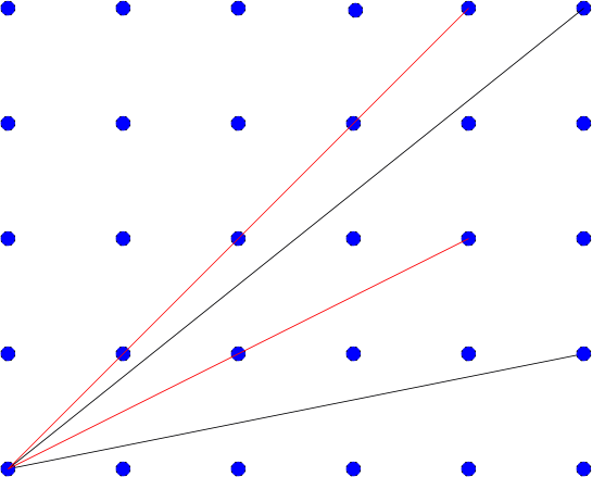
Figure 12. Black lines issued from the origin terminate at integer points with coprime coordinates; red lines terminate at integer points whose coordinates are not coprime

The Bourgain-Golse-Wennberg theorem raises the question, of whe- ther $\Phi_{r}(t)\simeq C/t$ in some sense as $r\to 0^{+}$ and $t\to+\infty$. Given the very different nature of the arguments used to establish the upper and the lower bounds in that theorem, this is a highly nontrivial problem, whose answer seems to be known only in space dimension $D=2$ so far. We shall return to this question later, and see that the $2$-dimensional situation is amenable to a class of very specific techniques based on continued fractions, that can be used to encode particle trajectories of the periodic Lorentz gas.

A first answer to this question, in space dimension $D=2$, is given by the following

Theorem 4.5 (Caglioti-Golse [9]).

Assume $D=2$ and define, for each $v\in\mathbf{S}^{1}$,

$$\phi_{r}(t|v)=\mu_{r}(\{x\in Z_{r}/\mathbf{Z}^{2}\,|\,\tau_{r}(x,v)\geq t/r\}\,,\quad t\geq 0\,.$$

Then there exists $\Phi:\,\mathbf{R}_{+}\to\mathbf{R}_{+}$ such that

$$\frac{1}{|\ln{\varepsilon}|}\int_{\varepsilon}^{1/4}\phi_{r}(t,v)\frac{dr}{r}\to\Phi(t)\hbox{ a.e. in }v\in\mathbf{S}^{1}$$

in the limit as ${\varepsilon}\to 0^{+}$. Moreover

$$\Phi(t)\sim\frac{1}{\pi^{2}t}\hbox{ as }t\to+\infty\,.$$

Shortly after [9] appeared, F. Boca and A. Zaharescu improved our method and managed to compute $\Phi(t)$ explicitly for each $t\geq 0$. One should keep in mind that their formula had been conjectured earlier by P. Dahlqvist [14], on the basis of a formal computation.

Theorem 4.6 (Boca-Zaharescu [3]).

For each $t>0$

$$\Phi_{r}(t)\to\Phi(t)=\int_{t}^{\infty}(s-t)g(s)ds$$

in the limit as $r\to 0^{+}$, where

$$g(s)=\tfrac{24}{\pi^{2}}\times\left\{\begin{matrix}1\quad&s\in[0,1]\,,\\ \tfrac{1}{s}+2\left(1-\tfrac{1}{s}\right)^{2}\ln(1-\tfrac{1}{s})-\tfrac{1}{2}\left|1-\tfrac{2}{s}\right|^{2}\ln|1-\tfrac{2}{s}|\quad&s\in(1,\infty)\,.\end{matrix}\right.$$

Figure 13. Graph of $\Phi(t)$ (right) and $g(t)=\Phi^{\prime\prime}(t)$ (left)

In the sequel, we shall return to the continued and Farey fractions techniques used in the proofs of these two results, and generalize them.

5. A negative result for the Boltzmann-Grad limit
of the periodic Lorentz gas

The material at our disposal so far provides us with a first answer — albeit a negative one — to the problem of determining the Boltzmann-Grad limit of the periodic Lorentz gas.

For simplicity, we consider the case of a Lorentz gas enclosed in a periodic box $\mathbf{T}^{D}=\mathbf{R}^{D}/\mathbf{Z}^{D}$ of unit side. The distance between neighboring obstacles is supposed to be ${\varepsilon}^{D-1}$ with $0<{\varepsilon}=1/n$, for $n\in\mathbf{N}$ and $n>2$ so that ${\varepsilon}<1/2$, while the obstacle radius is ${\varepsilon}^{D}<\tfrac{1}{2}{\varepsilon}^{D-1}$ — so that obstacles never overlap. Define

$$Y_{\varepsilon}=\{x\in\mathbf{T}^{D}\,|\,\hbox{dist}(x,{\varepsilon}^{D-1}\mathbf{Z}^{D})>{\varepsilon}^{D}\}={\varepsilon}^{D-1}(Z_{\varepsilon}/\mathbf{Z}^{D})\,.$$

For each $f^{in}\in C(\mathbf{T}^{D}\times\mathbf{S}^{D-1})$, let $f_{\varepsilon}$ be the solution of

$${\partial}_{t}f_{\varepsilon}+v\cdot{\nabla}_{x}f_{\varepsilon}=0\,, (x,v)\in Y_{\varepsilon}\times\mathbf{S}^{D-1}$$

$$f_{\varepsilon}(t,x,v)=f_{\varepsilon}(t,x,\mathcal{R}[n_{x}]v)\,, (x,v)\in{\partial}Y_{\varepsilon}\times\mathbf{S}^{D-1}$$

$$f_{\varepsilon}{\big{|}}_{t=0}=f^{in}\,,$$

where $n_{x}$ is unit normal vector to ${\partial}Y_{\varepsilon}$ at the point $x$, pointing towards the interior of $Y_{\varepsilon}$.

By the method of characteristics

$$f_{\varepsilon}(t,x,v)=f^{in}\left({\varepsilon}^{D-1}X_{\varepsilon}\left(-\tfrac{t}{{\varepsilon}^{D-1}};\tfrac{x}{{\varepsilon}^{D-1}},v\right);V_{\varepsilon}\left(-\tfrac{t}{{\varepsilon}^{D-1}};\tfrac{x}{{\varepsilon}^{D-1}},v\right)\right)$$

where $(X_{\varepsilon},V_{\varepsilon})$ is the billiard flow in $Z_{\varepsilon}$.

The main result in this section is the following

Theorem 5.1 (Golse [21, 24]).

There exist initial data $f^{in}\equiv f^{in}(x)\in C(\mathbf{T}^{D})$ such that no subsequence of $f_{\varepsilon}$ converges for the weak-* topology of $L^{\infty}(\mathbf{R}_{+}\times\mathbf{T}^{D}\times\mathbf{S}^{D-1})$ to the solution $f$ of a linear Boltzmann equation of the form

$$({\partial}_{t}+v\cdot{\nabla}_{x})f(t,x,v) ={\sigma}\int_{\mathbf{S}^{D-1}}p(v,v^{\prime})(f(t,x,v^{\prime})-f(t,x,v))dv^{\prime}$$

$$f{\big{|}}_{t=0} =f^{in}\,,$$

where ${\sigma}>0$ and $0\leq p\in L^{2}(\mathbf{S}^{D-1}\times\mathbf{S}^{D-1})$ satisfies

$$\int_{\mathbf{S}^{D-1}}p(v,v^{\prime})dv^{\prime}=\int_{\mathbf{S}^{D-1}}p(v^{\prime},v)dv^{\prime}=1\hbox{ a.e. in }v\in\mathbf{S}^{D-1}\,.$$

This theorem has the following important — and perhaps surprising — consequence: the Lorentz kinetic equation cannot govern the Boltzmann-Grad limit of the particle density in the case of a periodic distribution of obstacles.

Proof.

The proof of the negative result above involves two different arguments:

a) the existence of a spectral gap for any linear Boltzmann equation, and

b) the lower bound for the distribution of free path lengths in the Bourgain-Golse-Wennberg theorem.

Step 1: Spectral gap for the linear Boltzmann equation:

With ${\sigma}>0$ and $p$ as above, consider the unbounded operator $A$ on $L^{2}(\mathbf{T}^{D}\times\mathbf{S}^{D-1})$ defined by

$$(A\phi)(x,v)=-v\cdot{\nabla}_{x}\phi(x,v)-{\sigma}\phi(x,v)+{\sigma}\int_{\mathbf{S}^{D-1}}p(v,v^{\prime})\phi(x,v^{\prime})dv^{\prime}\,,$$

with domain

$$D(A)=\{\phi\in L^{2}(\mathbf{T}^{D}\times\mathbf{S}^{D-1})\,|\,v\cdot{\nabla}_{x}\phi\in L^{2}(\mathbf{T}^{D}\times\mathbf{S}^{D-1})\}\,.$$

Then

Theorem 5.2 (Ukai-Point-Ghidouche [45]).

There exists positive constants $C$ and ${\gamma}$ such that

$$\|e^{tA}\phi-\langle\phi\rangle\|_{L^{2}(\mathbf{T}^{D}\times\mathbf{S}^{D-1})}\leq Ce^{-{\gamma}t}\|\phi\|_{L^{2}(\mathbf{T}^{D}\times\mathbf{S}^{D-1})}\,,\quad t\geq 0\,,$$

for each $\phi\in L^{2}(\mathbf{T}^{D}\times\mathbf{S}^{D-1})$, where

$$\langle\phi\rangle=\tfrac{1}{|\mathbf{S}^{D-1}|}\iint_{\mathbf{T}^{D}\times\mathbf{S}^{D-1}}\phi(x,v)dxdv\,.$$

Taking this theorem for granted, we proceed to the next step in the proof, leading to an explicit lower bound for the particle density.

Step 2: Comparison with the case of absorbing obstacles

Assume that $f^{in}\equiv f^{in}(x)\geq 0$ on $\mathbf{T}^{D}$. Then

$$f_{\varepsilon}(t,x,v)\geq g_{\varepsilon}(t,x,v)=f^{in}(x-tv){\bf 1}_{Y_{\varepsilon}}(x){\bf 1}_{{\varepsilon}^{D-1}\tau_{\varepsilon}(x/{\varepsilon}^{D-1},v)>t}\,.$$

Indeed, $g$ is the density of particles with the same initial data as $f$, but assuming that each particle disappear when colliding with an obstacle instead of being reflected.

Then

$${\bf 1}_{Y_{\varepsilon}}(x)\to 1\hbox{ a.e. on $\mathbf{T}^{D}$ and }|{\bf 1}_{Y_{\varepsilon}}(x)|\leq 1$$

while, after extracting a subsequence if needed,

$${\bf 1}_{{\varepsilon}^{D-1}\tau_{\varepsilon}(x/{\varepsilon}^{D-1},v)>t}\rightharpoonup\Psi(t,v)\hbox{ in }L^{\infty}(\mathbf{R}_{+}\times\mathbf{T}^{D}\times\mathbf{S}^{D-1})\hbox{ weak-*}\,.$$

Therefore, if $f$ is a weak-* limit point of $f_{\varepsilon}$ in $L^{\infty}(\mathbf{R}_{+}\times\mathbf{T}^{D}\times\mathbf{S}^{D-1})$ as ${\varepsilon}\to 0$

$$f(t,x,v)\geq f^{in}(x-tv)\Psi(t,v)\hbox{ for a.e. }(t,x,v)\,.$$

Step 3: using the lower bound on the distribution of $\tau_{r}$

Denoting by $dv$ the uniform probability measure on $\mathbf{S}^{D-1}$

$$\tfrac{1}{|\mathbf{S}^{D-1}|}\iint_{\mathbf{T}^{D}\times\mathbf{S}^{D-1}} f(t,x,v)^{2}dxdv$$

$$\geq\tfrac{1}{|\mathbf{S}^{D-1}|}\iint_{\mathbf{T}^{D}\times\mathbf{S}^{D-1}}f^{in}(x-tv)^{2}\Psi(t,v)^{2}dxdv$$

$$=\int_{\mathbf{T}^{D}}f^{in}(y)^{2}dy\tfrac{1}{|\mathbf{S}^{D-1}|}\int_{\mathbf{S}^{D-1}}\Psi(t,v)^{2}dv$$

$$\geq\|f^{in}\|^{2}_{L^{2}(\mathbf{T}^{D})}\left(\tfrac{1}{|\mathbf{S}^{D-1}|}\int_{\mathbf{S}^{D-1}}\Psi(t,v)dv\right)^{2}$$

$$=\|f^{in}\|^{2}_{L^{2}(\mathbf{T}^{D})}\Phi(t)^{2}\,.$$

By the Bourgain-Golse-Wennberg lower bound on the distribution $\Phi$ of free path lengths

$$\|f(t,\cdot,\cdot)\|_{L^{2}(\mathbf{T}^{D}\times\mathbf{S}^{D-1})}\geq\frac{C_{D}}{t}\|f^{in}\|_{L^{2}(\mathbf{T}^{D})}\,,\quad t>1\,.$$

On the other hand, by the spectral gap estimate, if $f$ is a solution of the linear Boltzmann equation, one has

$$\|f(t,\cdot,\cdot)\|_{L^{2}(\mathbf{T}^{D}\times\mathbf{S}^{D-1})}\leq\int_{\mathbf{T}^{D}}f^{in}(y)dy+Ce^{-{\gamma}t}\|f^{in}\|_{L^{2}(\mathbf{T}^{D})}$$

so that

$$\frac{C_{D}}{t}\leq\frac{\|f^{in}\|_{L^{1}(\mathbf{T}^{D})}}{\|f^{in}\|_{L^{2}(\mathbf{T}^{D})}}+Ce^{-{\gamma}t}$$

for each $t>1$.

Step 4: choice of initial data

Pick $\rho$ to be a bump function supported near $x=0$ and such that

$$\int\rho(x)^{2}dx=1\,.$$

Take $f^{in}$ to be $x\mapsto{\lambda}^{D/2}\rho({\lambda}x)$ periodicized, so that

$$\int_{\mathbf{T}^{D}}f^{in}(x)^{2}dx=1\,,\hbox{ while }\int_{\mathbf{T}^{D}}f^{in}(y)dy={\lambda}^{-D/2}\int\rho(x)dx\,.$$

For such initial data, the inequality above becomes

$$\frac{C_{D}}{t}\leq{\lambda}^{-D/2}\int\rho(x)dx+Ce^{-{\gamma}t}\,.$$

Conclude by choosing ${\lambda}$ so that

$${\lambda}^{-D/2}\int\rho(x)dx<\sup_{t>1}\left(\frac{C_{D}}{t}-Ce^{-{\gamma}t}\right)>0\,.$$

∎

Remarks:

1) The same result (with the same proof) holds for any smooth obstacle shape included in a shell

$$\{x\in\mathbf{R}^{D}\,|\,C{\varepsilon}^{D}<\hbox{dist}(x,{\varepsilon}^{D-1}\mathbf{Z}^{D})<C^{\prime}{\varepsilon}^{D}\}\,.$$

2) The same result (with same proof) holds if the specular reflection boundary condition is replaced by more general boundary conditions, such as absorption (partial or complete) of the particles at the boundary of the obstacles, diffuse reflection, or any convex combination of specular and diffuse reflection — in the classical kinetic theory of gases, such boundary conditons are known as “accomodation boundary conditions”.

3) But introducing even the smallest amount of stochasticity in any periodic configuration of obstacles can again lead to a Boltzmann-Grad limit that is described by the Lorentz kinetic model.

Example. (Wennberg-Ricci [37]) In space dimension $2$, take obstacles that are disks of radius $r$ centered at the vertices of the lattice $r^{1/(2-\eta)}\mathbf{Z}^{2}$, assuming that $0<\eta<1$. Santaló’s formula suggests that the free-path lengths scale like $r^{\eta/(2-\eta)}\to 0$.

Suppose the obstacles are removed independently with large probability — specifically, with probability $p=1-r^{\eta/(2-\eta)}$. In that case, the Lorentz kinetic equation governs the 1-particle density in the Boltzmann-Grad limit as $r\to 0^{+}$.

Having explained why neither the Lorentz kinetic equation nor any linear Boltzmann equation can govern the Boltzmann-Grad limit of the periodic Lorentz gas, in the remaining part of these notes, we build the necessary material used in the description of that limit.

6. Coding particle trajectories with continued fractions

With the Bourgain-Golse-Wennberg lower bound for the distribution of free path lengths in the periodic Lorentz gas, we have seen that the $1$-particle phase space density is bounded below by a quantity that is incompatible with the spectral gap of any linear Boltzmann equation — in particular with the Lorentz kinetic equation.

In order to further analyze the Boltzmann-Grad limit of the periodic Lorentz gas, we cannot content ourselves with even more refined estimates on the distribution of free path lengths, but we need a convenient way to encode particle trajectories.

More precisely, the two following problems must be answered somehow:

First problem: for a particle leaving the surface of an obstacle in a given direction, to find the position of its next collision with an obstacle;

Second problem: average — in some sense to be defined — in order to eliminate the direction dependence.

From now on, our discussion is limited to the case of spatial dimension $D=2$, as we shall use continued fractions, a tool particularly well adapted to understanding the rational approximation of real numbers. Treating the case of a space dimension $D>2$ along the same lines would require a better understanding of simultaneous rational approximation of $D-1$ real numbers (by $D-1$ rational numbers with the same denominator), a notoriously more difficult problem.

We first introduce some basic geometrical objects used in coding particle trajectories.

The first such object is the notion of impact parameter.

For a particle with velocity $v\in\mathbf{S}^{1}$ located at the position $x$ on the surface of an obstacle (disk of radius $r$), we define its impact parameter $h_{r}(x,v)$ by the formula

$$h_{r}(x,v)=\sin(\widehat{n_{x},v})\,.$$

In other words, the absolute value of the impact parameter $h_{r}(x,v)$ is the distance of the center of the obstacle to the infinite line of direction $v$ passing through $x$ .

Obviously

$$h_{r}(x,\mathcal{R}[n_{x}]v)=h_{r}(x,v)$$

where we recall the notation $\mathcal{R}[n]v=v-2v\cdot nn$.

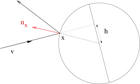
Figure 14. The impact parameter $h$ corresponding with the collision point $x$ at the surface of an obstacle, and a direction $v$

The next important object in computing particle trajectories in the Lorentz gas is the transfer map.

For a particle leaving the surface of an obstacle in the direction $v$ and with impact parameter $h^{\prime}$, define

$$T_{r}(h^{\prime},v)=(s,h)\hbox{ with }\left\{\begin{array}[]{l}s=\hbox{ $r\times$ distance to the next collision point}\\ h=\hbox{ impact parameter at the next collision}\end{array}\right.$$

Particle trajectories in the Lorentz gas are completely determined by the transfer map $T_{r}$ and its iterates.

Therefore, a first step in finding the Boltzmann-Grad limit of the periodic, $2$-dimensional Lorentz gas, is to compute the limit of $T_{r}$ as $r\to 0^{+}$, in some sense that will be explained later.

Figure 15. The transfer map

At first sight, this seems to be a desperately hard problem to solve, as particle trajectories in the periodic Lorentz gas depend on their directions and the obstacle radius in the strongest possible way. Fortunately, there is an interesting property of rational approximation on the real line that greatly reduces the complexity of this problem.

The 3-length theorem

Question (R. Thom, 1989): on a flat $2$-torus with a disk removed, consider a linear flow with irrational slope. What is the longest orbit?

Theorem 6.1 (Blank-Krikorian [1]).

On a flat $2$-torus with a segment removed, consider a linear flow with irrational slope $0<{\alpha}<1$. The orbits of this flow have at most $3$ different lengths — exceptionally $2$, but generically $3$. Moreover, in the generic case where these orbits have exactly $3$ different lengths, the length of the longest orbit is the sum of the two other lengths.

These lengths are expressed in terms of the continued fraction expansion of the slope ${\alpha}$.

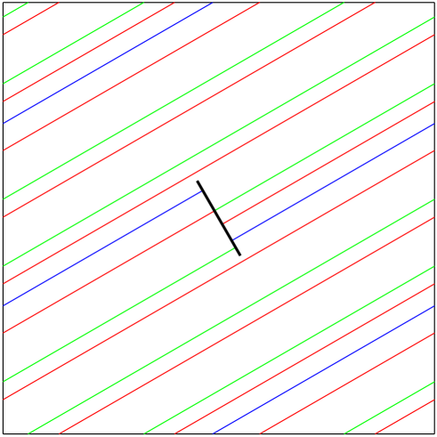
Figure 16. Three types of orbits: the blue orbit is the shortest, the red one is the longest, while the green one is of the intermediate length.The black segment removed is orthogonal to the direction of the trajectories.

Together with E. Caglioti in [9], we proposed the idea of using the Blank-Krikorian $3$-length theorem to analyze particle paths in the $2$-dimensional periodic Lorentz gas.

More precisely, orbits with the same lengths in the Blank-Krikorian theorem define a $3$-term partition of the flat $2$-torus into parallel strips, whose lengths and widths are computed exactly in terms of the continued fraction expansion of the slope (see Figure 17.)

The collision pattern for particles leaving the surface of one obstacle — and therefore the transfer map — can be explicitly determined in this way, for a.e. direction $v\in\mathbf{S}^{1}$.

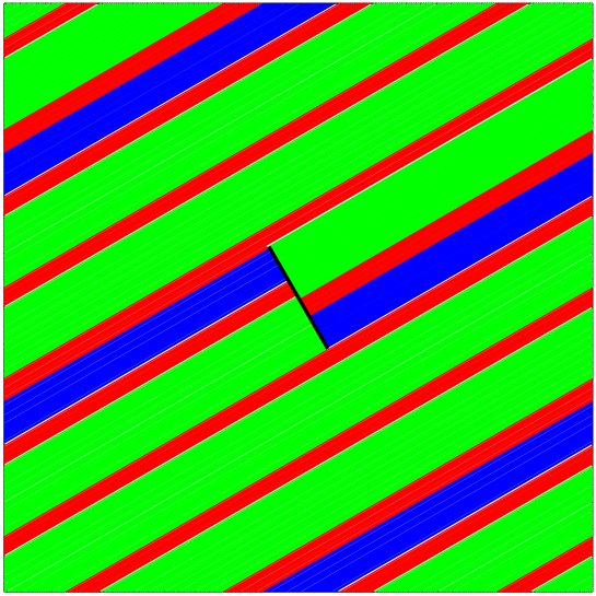
Figure 17. The $3$-term partition. The shortest orbits are collected in the blue strip, the longest orbits in the red strip, while the orbits of intermediate length are collected in the green strip.

In fact, there is a classical result known as the $3$-length theorem, which is related to Blank-Krikorian’s. Whereas the Blank-Krikorian theorem considers a linear flow with irrational slope on the flat $2$-torus, the classical $3$-length theorem is a statement about rotations of an irrational angle — i.e. about sections of the linear flow with irrational slope.

Theorem 6.2 ($3$-length theorem).

Let ${\alpha}\in(0,1)\setminus\mathbf{Q}$ and $N\geq 1$. The sequence

$$\{n{\alpha}\,|\,0\leq n\leq N\}$$

defines $N+1$ intervals on the circle of unit length $\simeq\mathbf{R}/\mathbf{Z}$. The lengths of these intervals take at most $3$ different values.

This striking result was conjectured by H. Steinhaus, and proved in 1957 independently by P. Erdös, G. Hajos, J. Suranyi, N. Swieczkowski, P. Szüsz — reported in [42], and by Vera Sòs [41].

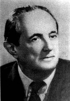
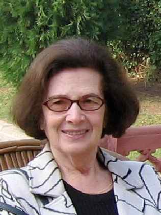
Figure 18. Left: Hugo D. Steinhaus (1887-1972); right: Vera T. Sós

As we shall see, the $3$-length theorem (in either form) is the key to encoding particle paths in the $2$-dimensional Lorentz gas. We shall need explicitly the formulas giving the lengths and widths of the $3$ strips in the partition of the flat $2$-torus defined by the Blank-Krikorian theorem. As this is based on the continued fraction expansion of the slope of the linear flow considered in the Blank-Krikorian theorem, we first recall some basic facts about continued fractions. An excellent reference for more information on this subject is [28].

Continued fractions

Assume $0<v_{2}<v_{1}$ and set ${\alpha}=v_{2}/v_{1}$, and consider the continued fraction expansion of ${\alpha}$:

$${\alpha}=[0;a_{0},a_{1},a_{2},\ldots]=\frac{1}{\displaystyle a_{0}+\frac{1}{\displaystyle a_{1}+\ldots}}\,.$$

Define the sequences of convergents $(p_{n},q_{n})_{n\geq 0}$ — meaning that

$$\frac{p_{n+2}}{q_{n+2}}=[0;a_{0},\ldots,a_{n}]\,,\quad n\geq 2$$

— by the recursion formulas

$$\begin{array}[]{ll}p_{n+1}=a_{n}p_{n}+p_{n-1}\,,&p_{0}=1\,,\,\,p_{1}=0\,,\\ q_{n+1}=a_{n}q_{n}+q_{n-1}&q_{0}=0\,,\,\,q_{1}=1\,.\end{array}$$

Finally, let $d_{n}$ denote the sequence of errors

$$d_{n}=|q_{n}\alpha-p_{n}|=(-1)^{n-1}(q_{n}{\alpha}-p_{n})\,,\quad n\geq 0\,,$$

so that

$$d_{n+1}=-a_{n}d_{n}+d_{n-1}\,,\quad d_{0}=1\,,\,\,d_{1}={\alpha}\,.$$

The sequence $d_{n}$ is decreasing and converges to $0$, at least exponentially fast. (In fact, the irrational number for which the rational approximation by continued fractions is the slowest is the one for which the sequence of denominators $q_{n}$ have the slowest growth, i.e. the golden mean

$${\theta}=[0;1,1,\ldots]=\frac{1}{1+\displaystyle\frac{1}{1+\ldots}}=\frac{\sqrt{5}-1}{2}\,.$$

The sequence of errors associated with ${\theta}$ satisfies $d_{n+1}=-d_{n}+d_{n-1}$ for each $n\geq 1$ with $d_{0}=1$ and $d_{1}={\theta}$, so that $d_{n}={\theta}^{n}$ for each $n\geq 0$.)

By induction, one verifies that

$$q_{n}d_{n+1}+q_{n+1}d_{n}=1\,,\quad n\geq 0\,.$$

Notation: we write $p_{n}({\alpha}),q_{n}({\alpha}),d_{n}({\alpha})$ to indicate the dependence of these quantities in ${\alpha}$.

Collision patterns

The Blank-Krikorian $3$-length theorem has the following consequence, of fundamental importance in our analysis.

Any particle leaving the surface of one obstacle in some irrational direction $v$ will next collide with one of at most $3$ — exceptionally 2 — other obstacles.

Any such collision pattern involving the $3$ obstacles seen by the departing particle in the direction of its velocity is completely determined by exactly $4$ parameters, computed in terms of the continued fraction expansion of $v_{2}/v_{1}$ — in the case where $0<v_{2}<v_{1}$, to which the general case can be reduced by obvious symmetry arguments.

Figure 19. Collision pattern seen from the surface of one obstacle. Here, ${\varepsilon}=2r/v_{1}$.

Assume therefore $0<v_{2}<v_{1}$ with ${\alpha}=v_{2}/v_{1}\notin\mathbf{Q}$. Henceforth, we set ${\varepsilon}=2r\sqrt{1+{\alpha}^{2}}$ and define

$$N(\alpha,{\varepsilon}) =\inf\{n\geq 0\,|\,d_{n}({\alpha})\leq{\varepsilon}\}\,,$$

$$k(\alpha,{\varepsilon}) =-\left[\frac{{\varepsilon}-d_{N(\alpha,{\varepsilon})-1}({\alpha})}{d_{N(\alpha,{\varepsilon})}({\alpha})}\right]\,.$$

The parameters defining the collision pattern are $A,B,Q$ — as they appear on the previous figure — together with an extra parameter ${\Sigma}\in\{\pm 1\}$. Here is how they are computed in terms of the continued fraction expansion of ${\alpha}=v_{2}/v_{1}$:

$$A(v,r) =1-\tfrac{d_{N({\alpha},{\varepsilon})}({\alpha})}{{\varepsilon}}\,,$$

$$B(v,r) =1-\tfrac{d_{N({\alpha},{\varepsilon})-1}({\alpha})}{{\varepsilon}}+\tfrac{k({\alpha},{\varepsilon})d_{N({\alpha},{\varepsilon})}({\alpha})}{{\varepsilon}}\,,$$

$$Q(v,r) ={\varepsilon}q_{N({\alpha},{\varepsilon})}({\alpha})\,,$$

$${\Sigma}(v,r) =(-1)^{N({\alpha},{\varepsilon})}\,.$$

The extra-parameter ${\Sigma}$ in the list above has the following geometrical meaning. It determines the relative position of the closest and next to closest obstacles seen from the particle leaving the surface of the obstacle at the origin in the direction $v$.

The case represented on the figure where the closest obstacle is on top of the strip consisting of the longest particle path corresponds with ${\Sigma}=+1$, the case where that obstacle is at the bottom of this same strip corresponds with ${\Sigma}=-1$.

The figure above showing one example of collision pattern involves still another parameter, denoted $Q^{\prime}$ on that figure.

This parameter $Q^{\prime}$ is not independent from $A,B,Q$, since one must have

$$AQ+BQ^{\prime}+(1-A-B)(Q+Q^{\prime})=1$$

each term in this sum corresponding to the surface of one of the three strips in the 3-term partition of the 2-torus. (Remember that the length of the longest orbit in the Blank-Krikorian theorem is the sum of the two other lengths.) Therefore

$$Q^{\prime}(v,r)=\frac{1-Q(v,r)(1-B(v,r))}{1-A(v,r)}\,.$$

Once the structure of collision patterns elucidated with the help of the Blank-Krikorian variant of the $3$-length theorem, we return to our original problem, namely that of computing the transfer map.

In the next proposition, we shall see that the transfer map in a given, irrational direction $v\in\mathbf{S}^{1}$ can be expressed explicitly in terms of the parameters $A,B,Q,{\Sigma}$ defining the collision pattern correponding with this direction.

Denote

$$\mathbf{K}:=]0,1[^{3}\times\{\pm 1\}$$

and let $(A,B,Q,{\Sigma})\in\mathbf{K}$ be the parameters defining the collision pattern seen by a particle leaving the surface of one obstacle in the direction $v$. Set

$$\begin{array}[]{rl}\mathbf{T}_{A,B,Q,{\Sigma}}(h^{\prime})=&(Q,h^{\prime}-2{\Sigma}(1-A))\\ \hbox{if }&1-2A<{\Sigma}h^{\prime}\leq 1\,,\\ \mathbf{T}_{A,B,Q,{\Sigma}}(h^{\prime})=&\left(Q^{\prime},h^{\prime}+2{\Sigma}(1-B)\right)\\ \hbox{if }&-1\leq{\Sigma}h^{\prime}<-1+2B\,,\\ \mathbf{T}_{A,B,Q,{\Sigma}}(h^{\prime})=&\left(Q^{\prime}+Q,h^{\prime}+2{\Sigma}(A-B)\right)\\ \hbox{if }&-1+2B\leq{\Sigma}h^{\prime}\leq 1-2A\,.\end{array}$$

With this notation, the transfer map is essentially given by the explicit formula $\mathbf{T}_{A,B,Q,{\Sigma}}$, except for an error of the order $O(r^{2})$ on the free-path length from obstacle to obstacle.

Proposition 6.3 (Caglioti-Golse [10, 11]).

One has

$$T_{r}(h^{\prime},v)=\mathbf{T}_{(A,B,Q,{\Sigma})(v,r)}(h^{\prime})+(O(r^{2}),0)$$

in the limit as $r\to 0^{+}$.

In fact, the proof of this proposition can be read on the figure above that represents a generic collision pattern. The first component in the explicit formula

$$\mathbf{T}_{(A,B,Q,{\Sigma})(v,r)}(h^{\prime})$$

represents exactly $r\times$ the distance between the vertical segments that are the projections of the diameters of the $4$ obstacles on the vertical ordinate axis. Obviously, the free-path length from obstacle to obstacle is the distance between the corresponding vertical segments, minus a quantity of the order $O(r)$ that is the distance from the surface of the obstacle to the corresponding vertical segment.

On the other hand, the second component in the same explicit formula is exact, as it relates impact parameters, which are precisely the intersections of the infinite line that contains the particle path with the vertical segments corresponding with the two obstacles joined by this particle path.

If we summarize what we have done so far, we see that we have solved our first problem stated at the beginning of the present section, namely that of finding a convenient way of coding the billiard flow in the periodic case and for space dimension $2$, for a.e. given direction $v$.

7. An ergodic theorem for collision patterns

It remains to solve the second problem, namely, to find a convenient way of averaging the computation above so as to get rid of the dependence on the direction $v$.

Before going further in this direction, we need to recall some known facts about the ergodic theory of continued fractions.

The Gauss map

Consider the Gauss map, which is defined on all irrational numbers in $(0,1)$ as follows:

$$T:\,(0,1)\setminus\mathbf{Q}\ni x\mapsto Tx=\tfrac{1}{x}-\left[\tfrac{1}{x}\right]\in(0,1)\setminus\mathbf{Q}\,.$$

This Gauss map has the following invariant probability measure — found by Gauss himself:

$$dg(x)=\tfrac{1}{\ln 2}\frac{dx}{1+x}\,.$$

Moreover, the Gauss map $T$ is ergodic for the invariant measure $dg(x)$. By Birkhoff’s theorem, for each $f\in L^{1}(0,1;dg)$

$$\frac{1}{N}\sum_{k=0}^{N-1}f(T^{k}x)\to\int_{0}^{1}f(z)dg(z)\hbox{ a.e. in }x\in(0,1)$$

as $N\to+\infty$.

How the Gauss map is related to continued fractions is explained as follows: for

$${\alpha}=[0;a_{0},a_{1},a_{2},\ldots]=\frac{1}{\displaystyle a_{0}+\frac{1}{\displaystyle a_{1}+\ldots}}\in(0,1)\setminus\mathbf{Q}$$

the terms $a_{k}({\alpha})$ of the continued fraction expansion of ${\alpha}$ can be computed from the iterates of the Gauss map acting on ${\alpha}$: specifically

$$a_{k}({\alpha})=\left[\frac{1}{T^{k}{\alpha}}\right]\,,\quad k\geq 0$$

As a consequence, the Gauss map corresponds with the shift to the left on infinite sequences of positive integers arising in the continued fraction expansion of irrationals in $(0,1)$. In other words,

$$T[0;a_{0},a_{1},a_{2},\ldots]=[0;a_{1},a_{2},a_{3}\ldots]\,,$$

equivalently recast as

$$a_{n}(T{\alpha})=a_{n+1}({\alpha})\,,\quad n\geq 0\,.$$

Thus, the terms $a_{k}({\alpha})$ of the continued fraction expansion of any ${\alpha}\in(0,1)\setminus\mathbf{Q}$ are easily expressed in terms of the sequence of iterates $(T^{k}{\alpha})_{k\geq 0}$ of the Gauss map acting on ${\alpha}$. The error $d_{n}({\alpha})$ is also expressed in term of that same sequence $(T^{k}{\alpha})_{k\geq 0}$, by equally simple formulas.

Starting from the induction relation on the error terms

$$d_{n+1}({\alpha})=-a_{n}({\alpha})d_{n}({\alpha})+d_{n-1}({\alpha})\,,\quad d_{0}({\alpha})=1\,,\,\,d_{1}({\alpha})={\alpha}$$

and the explicit formula relating $a_{n}(T{\alpha})$ to $a_{n}({\alpha})$, we see that

$${\alpha}d_{n}(T{\alpha})=d_{n+1}({\alpha})\,,\quad n\geq 0\,.$$

This entails the formula

$$d_{n}({\alpha})=\prod_{k=0}^{n-1}T^{k}{\alpha}\,,\quad n\geq 0\,.$$

Observe that, for each ${\theta}\in[0,1]\setminus\mathbf{Q}$, one has

$${\theta}\cdot T{\theta}<\tfrac{1}{2}\,,$$

so that

$$d_{n}({\alpha})\leq 2^{-[n/2]}\,,\quad n\geq 0\,,$$

which establishes the exponential decay mentionned above. (As a matter of fact, exponential convergence is the slowest possible for the continued fraction algorithm, as it corresponds with the rational approximation of algebraic numbers of degree $2$, which are the hardest to approximate by rational numbers.)

Unfortunately, the dependence of $q_{n}({\alpha})$ in ${\alpha}$ is more complicated. Yet one can find a way around this, with the following observation. Starting from the relation

$$q_{n+1}({\alpha})d_{n}({\alpha})+q_{n}({\alpha})d_{n+1}({\alpha})=1\,,$$

we see that

$$q_{n}({\alpha})d_{n-1}({\alpha}) =\sum_{j=1}^{n}(-1)^{n-j}\frac{d_{n}({\alpha})d_{n-1}({\alpha})}{d_{j}({\alpha})d_{j-1}({\alpha})}$$

$$=\sum_{j=1}^{n}(-1)^{n-j}\prod_{k=j}^{n-1}T^{k-1}{\alpha}T^{k}{\alpha}\,.$$

Using once more the inequality ${\theta}\cdot T{\theta}<\tfrac{1}{2}$ for ${\theta}\in[0,1]\setminus\mathbf{Q}$, one can truncate the summation above at the cost of some exponentially small error term. Specifically, one finds that

$$\left|q_{n}({\alpha})d_{n-1}({\alpha})-\sum_{j=n-l}^{n}(-1)^{n-j}\frac{d_{n}({\alpha})d_{n-1}({\alpha})}{d_{j}({\alpha})d_{j-1}({\alpha})}\right|$$

$$\qquad=\left|q_{n}({\alpha})d_{n-1}({\alpha})-\sum_{j=n-l}^{n}(-1)^{n-j}\prod_{k=j}^{n-1}T^{k-1}{\alpha}T^{k}{\alpha}\right|\leq 2^{-l}\,.$$

More information on the ergodic theory of continued fractions can be found in the classical monograph [28] on continued fractions, and in Sinai’s book on ergodic theory [40].

An ergodic theorem

We have seen in the previous section that the transfer map satisfies

$$T_{r}(h^{\prime},v)=\mathbf{T}_{(A,B,Q,{\Sigma})(v,r)}(h^{\prime})+(O(r^{2}),0)\hbox{ as }r\to 0^{+}$$

for each $v\in\mathbf{S}^{1}$ such that $v_{2}/v_{1}\in(0,1)\setminus\mathbf{Q}$.

Obviously, the parameters $(A,B,Q,{\Sigma})$ are extremely sensitive to variations in $v$ and $r$ as $r\to 0^{+}$, so that even the explicit formula for $T_{A,B,Q,{\Sigma}}$, is not too useful in itself.

Each time one must handle a strongly oscillating quantity such as the free path length $\tau_{r}(x,v)$ or the transfer map $T_{r}(h^{\prime},v)$, it is usually a good idea to consider the distribution of that quantity under some natural probability measure than the quantity itself. Following this principle, we are led to consider the family of probability measures in $(s,h)\in\mathbf{R}_{+}\times[-1,1]$

$${\delta}((s,h)-T_{r}(h^{\prime},v))\,,$$

or equivalently

$${\delta}((s,h)-T_{(A,B,Q,{\Sigma})(v,r)}(h^{\prime}))\,.$$

A first obvious idea would be to average out the dependence in $v$ of this family of measures: as we shall see later, this is not an easy task.

A somewhat less obvious idea is to average over obstacle radius. Perhaps surprisingly, this is easier than averaging over the direction $v$.

That averaging over obstacle radius is a natural operation in this context can be explained by the following observation. We recall that the sequence of errors $d_{n}({\alpha})$ in the continued fraction expansion of an irrational ${\alpha}\in(0,1)$ satisfies

$${\alpha}d_{n}(T{\alpha})=d_{n+1}({\alpha})\,,\quad n\geq 0\,,$$

so that

$$N({\alpha},{\varepsilon})=\inf\{n\geq 1\,|\,d_{n}({\alpha})\leq{\varepsilon}\}$$

is transformed by the Gauss map as follows:

$$N(a,{\varepsilon})=N(T{\alpha},{\varepsilon}/{\alpha})+1\,.$$

In other words, the transfer map for the $2$-dimensional periodic Lorentz gas in the billiard table $Z_{r}$ (meaning, with circular obstacles of radius $r$ centered at the vertices of the lattice $\mathbf{Z}^{2}$) in the direction $v$ corresponding with the slope ${\alpha}$ is essentially the same as for the billiard table $Z_{r/{\alpha}}$ but in the direction corresponding with the slope $T{\alpha}$. Since the problem is invariant under the transformation

$${\alpha}\mapsto T{\alpha}\,,\qquad r\mapsto r/{\alpha}$$

this suggests the idea of averaging with respect to the scale invariant measure in the variable $r$, i.e. $\frac{dr}{r}$ on $\mathbf{R}_{+}^{*}$.

The key result in this direction is the following ergodic lemma for functions that depend on finitely many $d_{n}$s.

Lemma 7.1 (Caglioti-Golse [9, 22, 11]).

For ${\alpha}\in(0,1)\setminus\mathbf{Q}$, set

$$N({\alpha},{\varepsilon})=\inf\{n\geq 0\,|\,d_{n}({\alpha})\leq{\varepsilon}\}\,.$$

For each $m\geq 0$ and each $f\in C(\mathbf{R}_{+}^{m+1})$, one has

$$\frac{1}{|\ln\eta|}\int_{\eta}^{1/4}f\left(\frac{d_{N({\alpha},{\varepsilon})}({\alpha})}{{\varepsilon}},\ldots,\frac{d_{N({\alpha},{\varepsilon})-m}({\alpha})}{{\varepsilon}}\right)\frac{d{\varepsilon}}{{\varepsilon}}\to L_{m}(f)$$

a.e. in ${\alpha}\in(0,1)$ as $\eta\to 0^{+}$, where the limit $L_{m}(f)$ is independent of ${\alpha}$.

With this lemma, we can average over obstacle radius any function that depends on collision patterns, i.e. any function of the parameters $A,B,Q,{\Sigma}$.

Proposition 7.2 (Caglioti-Golse [11]).

Let $\mathbf{K}=[0,1]^{3}\times\{\pm 1\}$. For each $F\in C(\mathbf{K})$, there exists $\mathcal{L}(F)\in\mathbf{R}$ independent of $v$ such that

$$\frac{1}{\ln(1/\eta)}\int_{\eta}^{1/2}F(A(v,r),B(v,r),Q(v,r),{\Sigma}(v,r))\frac{dr}{r}\to\mathcal{L}(F)$$

for a.e. $v\in\mathbf{S}^{1}$ such that $0<v_{2}<v_{1}$ in the limit as $\eta\to 0^{+}$.

Sketch of the proof.

First eliminate the ${\Sigma}$ dependence by decomposing

$$F(A,B,Q,{\Sigma})=F_{+}(A,B,Q)+{\Sigma}F_{-}(A,B,Q)\,.$$

Hence it suffices to consider the case where $F\equiv F(A,B,Q)$.

Setting ${\alpha}=v_{2}/v_{1}$ and ${\varepsilon}=2r/v_{1}$, we recall that

$$A(v,r) \hbox{ is a function of }\frac{d_{N({\alpha},{\varepsilon})}({\alpha})}{{\varepsilon}}\,,$$

$$B(v,r) \hbox{ is a function of }\frac{d_{N({\alpha},{\varepsilon})}({\alpha})}{{\varepsilon}}\hbox{ and }\frac{d_{N({\alpha},{\varepsilon})-1}({\alpha})}{{\varepsilon}}\,.$$

As for the dependence of $F$ on $Q$, proceed as follows: in $F(A,B,Q)$, replace $Q(v,r)$ with

$$\frac{{\varepsilon}}{d_{N({\alpha},{\varepsilon})-1}}\sum_{j=N({\alpha},{\varepsilon})-l}^{N({\alpha},{\varepsilon})}(-1)^{{N({\alpha},{\varepsilon})}-j}\frac{d_{N({\alpha},{\varepsilon})}({\alpha})d_{{N({\alpha},{\varepsilon})}-1}({\alpha})}{d_{j}({\alpha})d_{j-1}({\alpha})}\,,$$

at the expense of an error term of the order

$$O(\hbox{modulus of continuity of $F$}(2^{-m}))\to 0\hbox{ as }l\to 0\,,$$

uniformly as ${\varepsilon}\to 0^{+}$.

This substitution leads to an integrand of the form

$$f\left(\frac{d_{N({\alpha},{\varepsilon})}({\alpha})}{{\varepsilon}},\ldots,\frac{d_{N({\alpha},{\varepsilon})-m-1}({\alpha})}{{\varepsilon}}\right)$$

to which we apply the ergodic lemma above: its Cesàro mean converges, in the small radius limit, to some limit $\mathcal{L}_{m}(F)$ independent of ${\alpha}$.

By uniform continuity of $F$, one finds that

$$|\mathcal{L}_{m}(F)-\mathcal{L}_{m^{\prime}}(F)|=O(\hbox{modulus of continuity of $F$}(2^{-m\vee m^{\prime}}))$$

(with the notation $m\vee m^{\prime}=\max(v,v^{\prime})$), so that $\mathcal{L}_{m}(F)$ is a Cauchy sequence as $m\to\infty$. Hence

$$\mathcal{L}_{m}(F)\to\mathcal{L}(F)\hbox{ as }m\to\infty$$

and with the error estimate above for the integrand, one finds that

$$\frac{1}{\ln(1/\eta)}\int_{\eta}^{1/2}F(A(v,r),B(v,r),Q(v,r),{\Sigma}(v,r))\frac{dr}{r}\to\mathcal{L}(F)$$

as $\eta\to 0^{+}$. ∎

With the ergodic theorem above, and the explicit approximation of the transfer map expressed in terms of the parameters $(A,B,Q,{\Sigma})$ that determine collision patterns in any given direction $v$, we easily arrive at the following notion of a “probability of transition” for a particle leaving the surface of an obstacle with an impact parameter $h^{\prime}$ to hit the next obstacle on its trajectory at time $s/r$ with an impact parameter $h$.

Theorem 7.3 (Caglioti-Golse, [10, 11]).

For each $h^{\prime}\in[-1,1]$, there exists a probability density $P(s,h|h^{\prime})$ on $\mathbf{R}_{+}\times[-1,1]$ such that, for each $f\in C(\mathbf{R}_{+}\times[-1,1])$,

$$\frac{1}{|\ln\eta|}\int_{\eta}^{1/4}f(T_{r}(h^{\prime},v))\frac{dr}{r}\to\int_{0}^{\infty}\int_{-1}^{1}f(s,h)P(s,h|h^{\prime})dsdh$$

a.e. in $v\in\mathbf{S}^{1}$ as $\eta\to 0^{+}$.

In other words, the transfer map converges in distribution and in the sense of Cesàro, in the small radius limit, to a transition probability $P(s,h|h^{\prime})$ that is independent of $v$.

We are therefore left with the following problems:

a) to compute the transition probability $P(s,h|h^{\prime})$ explicitly and discuss its properties, and

b) to explain the role of this transition probability in the Boltzmann-Grad limit of the periodic Lorentz gas dynamics.

8. Explicit computation
of the transition probability $P(s,h|h^{\prime})$

Most unfortunately, our argument leading to the existence of the limit $\mathcal{L}(F)$, the core result of the previous section, cannot be used for computing explicitly the value $\mathcal{L}(F)$. Indeed, the convergence proof is based on the ergodic lemma in the last section, coupled to a sequence of approximations of the parameter $Q$ in collision patterns that involve only finitely many error terms $d_{n}({\alpha})$ in the continued fraction expansion of ${\alpha}$. The existence of the limit is obtained through Cauchy’s criterion, precisely because of the difficulty in finding an explicit expression for the limit.

Nevertheless, we have arrived at the following expression for the transition probability $P(s,h|h^{\prime})$:

Theorem 8.1 (Caglioti-Golse [10, 11]).

The transition probability density $P(s,h|h^{\prime})$ is expressed in terms of $a=\tfrac{1}{2}|h-h^{\prime}|$ and $b=\tfrac{1}{2}|h+h^{\prime}|$ by the explicit formula

$$P(s,h|h^{\prime})=\frac{3}{\pi^{2}sa}\Big{[}\left((s-\tfrac{1}{2}sa)\!\wedge\!(1+\tfrac{1}{2}sa)\!-\!(1\!\vee\!(\tfrac{1}{2}s+\tfrac{1}{2}sb)\right)_{+}$$

$$+\!\left((s-\textstyle\frac{1}{2}sa)\!\wedge\!1\!-\!((\tfrac{1}{2}s+\tfrac{1}{2}sb)\!\vee\!\left(1\!-\!\textstyle\frac{1}{2}sa\right)\right)_{+}$$

$$\!+\!sa\!\wedge\!|1-s|\mathbf{1}_{s<1}+(sa\!-\!|1-s|)_{+}\Big{]}\,,$$

with the notations $x\wedge y=\min(x,y)$ and $x\vee y=\max(x,y)$.

Moreover, the function

$$(s,h,h^{\prime})\mapsto(1+s)P(s,h|h^{\prime})\hbox{ belongs to }L^{2}(\mathbf{R}_{+}\times[-1,1]^{2})\,.$$

In fact, the key result in the proof of this theorem is the asymptotic distribution of $3$-obstacle collision patterns — i.e. the computation of the limit $\mathcal{L}(f)$, whose existence has been proved in the last section’s proposition.

Theorem 8.2 (Caglioti-Golse [11]).

Define $\mathbf{K}=[0,1]^{3}\times\{\pm 1\}$; then, for each $F\in C(\mathbf{K})$

$$\frac{1}{|\ln\eta|}\int_{\eta}^{1/4}F((A,B,Q,{\Sigma})(v,r))\frac{dr}{r}\to\mathcal{L}(F)$$

$$=\int_{\mathbf{K}}F(A,B,Q,{\Sigma})dm(A,B,Q,{\Sigma})\hbox{ a.e. in }v\in\mathbf{S}^{1}$$

as $\eta\to 0^{+}$, where

$$dm(A,B,Q,{\Sigma}) =dm_{0}(A,B,Q)\otimes\tfrac{1}{2}({\delta}_{{\Sigma}=1}+{\delta}_{{\Sigma}=-1})\,,$$

$$dm_{0}(A,B,Q) =\tfrac{12}{\pi^{2}}{\bf 1}_{0<A<1}{\bf 1}_{0<B<1-A}{\bf 1}_{0<Q<\frac{1}{2-A-B}}\frac{dAdBdQ}{1-A}\,.$$

Before giving an idea of the proof of the theorem above on the distribution of $3$-obstacle collision patterns, it is perhaps worthwhile explaining why the measure $m$ above is somehow natural in the present context.

To begin with, the constraints $0<A<1$ and $0<B<1-A$ have an obvious geometric meaning (see figure 18 on collision patterns.) More precisely, the widths of the three strips in the $3$-term partition of the $2$-torus minus the slit constructed in the penultimate section (as a consequence of the Blank-Krikorian $3$-length theorem) add up to $1$. Since $A$ is the width of the strip consisting of the shortest orbits in the Blank-Krikorian theorem, and $B$ that of the strip consisting of the next to shortest orbits, one has

$$0<A+B\leq 1$$

with equality only in the exceptional case where the orbits have at most $2$ different lengths, which occurs for a set of measure $0$ in $v$ or $r$. Therefore, one has

$$0<B(v,r)<1-A(v,r)\,,\quad\hbox{ for a.e. }r\in(0,\tfrac{1}{2})\,.$$

Likewise, the total area of the $2$-torus is the sum of the areas of the strips consisting of all orbits with the $3$ possible lengths:

$$1=QA+Q^{\prime}B+(Q+Q^{\prime})(1-A-B) =Q(1-B)+Q^{\prime}(1-A)$$

$$\geq Q(2-A-B)$$

as $Q^{\prime}\geq Q$ (see again the figure above on collision patterns.)

Therefore, the volume element

$$\frac{dAdBdQ}{1-A}$$

in the expression of $dm_{0}$ imples that the parameters $A$, $\frac{B}{1-A}$ — or equivalently $B$ mod. $1-A$ — and $Q$ are independent and uniformly distributed in the largest subdomain of $[0,1]^{3}$ that is compatible with the geometric constraints.

The first theorem is a consequence of the second: indeed, $P(s,h|h^{\prime})dsdh$ is the image measure of $dm(A,B,Q,{\Sigma})$ under the map

$$\mathbf{K}\ni(A,B,Q,{\Sigma})\mapsto T_{(A,B,Q,{\Sigma})}(h^{\prime},v)\,.$$

That $(1+s)P(s,h|h^{\prime})$ is square integrable is proved by inspection — by using the explicit formula for $P(s,h|h^{\prime})$.

Therefore, it remains to prove the second theorem.

We are first going to show that the family of averages over velocities satisfy

$$\int_{|v|=1\atop 0<v_{2}<v_{1}} F(A(v,r),B(v,r),Q(v,r),{\Sigma}(v,r))dv$$

$$\to\tfrac{\pi}{8}\int_{\mathbf{K}}F(A,B,Q,{\Sigma})dm(A,B,Q,{\Sigma})$$

as $r\to 0^{+}$ for each $F\in C_{b}(\mathbf{K})$.

On the other hand, because of the proposition in the previous section

$$\frac{1}{\ln(1/\eta)}\int_{\eta}^{1/2}F(A(v,r),B(v,r),Q(v,r),{\Sigma}(v,r))\frac{dr}{r}\to\mathcal{L}(F)$$

for a.e. $v\in\mathbf{S}^{1}$ such that $0<v_{2}<v_{1}$ in the limit as $\eta\to 0^{+}$.

Since we know that the limit $\mathcal{L}(F)$ is independent of $v$, comparing the two convergence statements above shows that

$$\mathcal{L}(F)=\int_{\mathbf{K}}F(A,B,Q,{\Sigma})dm(A,B,Q,{\Sigma})\,.$$

Therefore, we are left with the task of computing

$$\lim_{r\to 0^{+}}\int_{|v|=1\atop 0<v_{2}<v_{1}}F(A(v,r),B(v,r),Q(v,r),{\Sigma}(v,r))dv\,.$$

The method for computing this type of expression is based on

a) Farey fractions (sometimes called “slow continued fractions”), and

b) estimates for Kloosterman’s sums, due to Boca-Zaharescu [3].

To begin with, we need to recall a few basic facts about Farey fractions.

Farey fractions

Put a filtration on the set of rationals in $[0,1]$ as follows

$$\mathcal{F}_{\mathcal{Q}}=\{\tfrac{p}{q}\,|\,0\leq p\leq q\leq\mathcal{Q}\,,\,\,\hbox{g.c.d.}(p,q)=1\}$$

indexed in increasing order:

$$0=\frac{0}{1}<{\gamma}_{1}<\ldots<{\gamma}_{j}=\frac{p_{j}}{q_{j}}<\ldots<{\gamma}_{\varphi(\mathcal{Q})}=\frac{1}{1}=1$$

where $\varphi$ denotes Euler’s totient function:

$$\phi(n)=n\prod_{p\hbox{ \tiny{prime} }\atop p|n}\left(1-\frac{1}{p}\right)\,.$$

An important operation in the construction of Farey fractions is the notion of “mediant” of two fractions. Given two rationals

$${\gamma}=\frac{p}{q}\hbox{ and }\hat{\gamma}=\frac{\hat{p}}{\hat{q}}$$

with

$$0\leq p\leq q\,,\quad 0\leq\hat{p}\leq\hat{q}\,,\hbox{ and }\hbox{ g.c.d.}(p,q)=\hbox{ g.c.d.}(\hat{p},\hat{q})=1\,,$$

their mediant is defined as

$$\hbox{mediant}={\gamma}\oplus\hat{\gamma}:=\frac{p+\hat{p}}{q+\hat{q}}\in({\gamma},\hat{\gamma})\,.$$

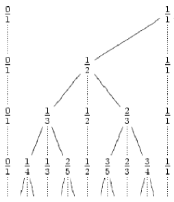
Figure 20. The Stern-Brocot tree. Each fraction ${\gamma}$ on the $n$-th line is the mediant of the two fractions closest to ${\gamma}$ on the $n-1$-st line. The first line consists of $0$ and $1$ written as $0=\frac{0}{1}$ and $1=\frac{1}{1}$. Each rational in $[0,1]$ is obtained in this way.

Hence, if ${\gamma}=\frac{p}{q}<\hat{\gamma}=\frac{\hat{p}}{\hat{q}}$ adjacent in $\mathcal{F}_{\mathcal{Q}}$, then

$$\hat{a}q-a\hat{q}=1\hbox{ and }q+\hat{q}>\mathcal{Q}\,.$$

Conversely, $q,\hat{q}$ are denominators of adjacent fractions in $\mathcal{F}_{\mathcal{Q}}$ if and only if

$$0\leq q,\hat{q}\leq\mathcal{Q}\,,\quad q+\hat{q}>\mathcal{Q}\,,\quad\hbox{g.c.d.}(q,q^{\prime})=1\,.$$

Given ${\alpha}\in(0,1)\setminus\mathbf{Q}$ and $\mathcal{Q}\geq 1$, there exists a unique pair of adjacent Farey fractions in $\mathcal{F}_{\mathcal{Q}}$, henceforth denoted ${\gamma}({\alpha},\mathcal{Q})$ and $\hat{\gamma}({\alpha},\mathcal{Q})$, such that

$${\gamma}({\alpha},\mathcal{Q})=\frac{p({\alpha},\mathcal{Q})}{q({\alpha},\mathcal{Q})}<{\alpha}<\hat{\gamma}({\alpha},\mathcal{Q})=\frac{\hat{p}({\alpha},\mathcal{Q})}{\hat{q}({\alpha},\mathcal{Q})}\,.$$

At this point, we recall the relation between Farey and continued fractions.

Pick $0<{\varepsilon}<1$; we recall that, for each ${\alpha}\in(0,1)\setminus\mathbf{Q}$,

$$N({\alpha},{\varepsilon})=\min\{n\in\mathbf{N}\,|\,d_{n}({\alpha})\leq{\varepsilon}\}\,,\quad d_{n}({\alpha})=\hbox{dist}(q_{n}({\alpha}){\alpha},\mathbf{Z})\,.$$

Set $\mathcal{Q}=[1/{\varepsilon}]$, and let

$${\gamma}({\alpha},\mathcal{Q})=\frac{p({\alpha},\mathcal{Q}))}{q({\alpha},\mathcal{Q})}<\hat{\gamma}({\alpha},\mathcal{Q})=\frac{\hat{p}({\alpha},\mathcal{Q}))}{\hat{q}({\alpha},\mathcal{Q})}$$

with $g.c.d.(p({\alpha},\mathcal{Q})),q({\alpha},\mathcal{Q}))=g.c.d.(\hat{p}({\alpha},\mathcal{Q})),\hat{q}({\alpha},\mathcal{Q}))=1$ be the two adjacent Farey fractions in $\mathcal{F}_{\mathcal{Q}}$ surrounding ${\alpha}$. Then

a) one of the two integers $q({\alpha},\mathcal{Q})$ and ${\hat{q}({\alpha},\mathcal{Q})}$ is the denominator of the $N({\alpha},{\varepsilon})$-th convergent in the continued fraction expansion of ${\alpha}$, i.e. $q_{N({\alpha},{\varepsilon})}({\alpha})$, and

b) the other is of the form

$$mq_{N({\alpha},{\varepsilon})}+q_{N({\alpha},{\varepsilon})-1}\,,\quad\hbox{ with }0\leq m\leq a_{N({\alpha},{\varepsilon})}({\alpha})\,,$$

where we recall that

$${\alpha}=[0;a_{1},a_{2},\ldots]=\frac{1}{a_{0}+\displaystyle\frac{1}{a_{1}+\ldots}}\,.$$

Setting ${\alpha}=v_{2}/v_{1}$ and ${\varepsilon}=2r/v_{1}$, we recall that, by definition

$$Q(v,r)={\varepsilon}q_{N({\alpha},{\varepsilon})}({\alpha})\in\{{\varepsilon}q({\alpha},\mathcal{Q}),{\varepsilon}\hat{q}({\alpha},\mathcal{Q})\}\hbox{ with }\mathcal{Q}=[1/{\varepsilon}]\,,$$

and we further define

$$D(v,r)=d_{N({\alpha},{\varepsilon})}/{\varepsilon}=\hbox{dist}(\tfrac{1}{{\varepsilon}}Q(v,r){\alpha},\mathbf{Z})/{\varepsilon}\,,$$

and

$$\tilde{Q}(v,r)={\varepsilon}\hat{q}({\alpha},\mathcal{Q})\hbox{ if }q_{N({\alpha},{\varepsilon})}({\alpha})=q({\alpha},\mathcal{Q})\,,$$

$$\tilde{Q}(v,r)={\varepsilon}q({\alpha},\mathcal{Q})\hbox{ if }q_{N({\alpha},{\varepsilon})}({\alpha})=\hat{q}({\alpha},\mathcal{Q})\,.$$

Now, we recall that $A(v,r)=1-D(v,r)$; moreover, we see that

$$B(v,r) =1-\frac{d_{N({\alpha},{\varepsilon})-1}({\alpha})}{{\varepsilon}}-\left[\frac{1-d_{N({\alpha},{\varepsilon})-1}({\alpha})/{\varepsilon}}{D(v,r)}\right]D(v,r)$$

$$=1-d_{N({\alpha},{\varepsilon})-1}({\alpha})/{\varepsilon}\hbox{ mod. }D(v,r)$$

$$=1-\hbox{dist}(\tfrac{1}{{\varepsilon}}\tilde{Q}(v,r){\alpha},\mathbf{Z})/{\varepsilon}\hbox{ mod. }D(v,r)\,.$$

To summarize, we have

$$F(A(v,r),B(v,r),Q(v,r))=G(Q(v,r),\tilde{Q}(v,r),D(v,r))$$

and we are left with the task of computing

$$\lim_{r\to 0^{+}}\int_{\mathbf{S}_{+}^{1}}G(Q(v,r),\tilde{Q}(v,r),D(v,r))dv$$

where $\mathbf{S}^{1}_{+}$ is the first octant in the unit circle. The other octants in the unit circle give the same contribution by obvious symmetry arguments.

More specifically:

Lemma 8.3.

Let ${\alpha}\in(0,1)\setminus\mathbf{Q}$, and let $\tfrac{p}{q}<{\alpha}<\tfrac{\hat{p}}{\hat{q}}$ be the two adjacent Farey fractions in $\mathcal{F}_{\mathcal{Q}}$ surrounding ${\alpha}$, with $\mathcal{Q}=[1/{\varepsilon}]$. Then

a) if $\frac{p}{q}<{\alpha}\leq\frac{\hat{p}-{\varepsilon}}{\hat{q}}$, then

$$Q(v,r)={\varepsilon}q\,,\quad\tilde{Q}(v,r)={\varepsilon}\hat{q}\,,\quad D(v,r)=\tfrac{1}{{\varepsilon}}({\alpha}q-p)\,;$$

b) if $\frac{p+{\varepsilon}}{q}<{\alpha}<\frac{\hat{p}}{\hat{q}}$, then

$$Q(v,r)={\varepsilon}\hat{q}\,,\quad\tilde{Q}(v,r)={\varepsilon}q\,,\quad D(v,r)=\tfrac{1}{{\varepsilon}}(\hat{p}-{\alpha}\hat{q})\,;$$

c) if $\frac{p+{\varepsilon}}{q}<{\alpha}\leq\frac{\hat{p}-{\varepsilon}}{\hat{q}}$, then

$$Q(v,r)={\varepsilon}(q\wedge\hat{q})\,,\quad\tilde{Q}(v,r)={\varepsilon}(q\vee\hat{q})\,,\quad D(v,r)=\hbox{dist}(\tfrac{1}{{\varepsilon}}Q(v,r){\alpha},\mathbf{Z})\,.$$

Therefore, assuming for simplicity that

$$G(x,y,z)=g(x,y)H^{\prime}(z)\hbox{ and }{\varepsilon}=1/\mathcal{Q}\,,$$

one has

$$\int_{\mathbf{S}_{+}^{1}}G(Q(v,r),\hat{Q}(v,r),D(v,r))dv$$

$$=\sum_{0<q,\hat{q}\leq\mathcal{Q}<q+\hat{q}\atop g.c.d.(q,\hat{q})=1}\int_{p/q}^{(\hat{p}-{\varepsilon})/\hat{q}}g\left(\frac{q}{\mathcal{Q}},\frac{\hat{q}}{\mathcal{Q}}\right)H^{\prime}(\mathcal{Q}(q{\alpha}-p))d{\alpha}$$

$$+\hbox{ three other similar terms }$$

$$=\sum_{0<q,\hat{q}\leq\mathcal{Q}<q+\hat{q}\atop g.c.d.(q,\hat{q})=1}g\left(\frac{q}{\mathcal{Q}},\frac{\hat{q}}{\mathcal{Q}}\right)\frac{1}{q\mathcal{Q}}\left(H\left(\frac{1-q/\mathcal{Q}}{\hat{q}/\mathcal{Q}}\right)-H(0)\right)$$

$$+\hbox{ three other similar terms.}$$

Then, everything reduces to computing

$$\lim_{\mathcal{Q}\to+\infty}\frac{1}{\mathcal{Q}^{2}}\sum_{0<q,\hat{q}\leq\mathcal{Q}<q+\hat{q}\atop g.c.d.(q,\hat{q})=1}\psi\left(\frac{q}{\mathcal{Q}},\frac{\hat{q}}{\mathcal{Q}}\right)\,.$$

We conclude with the following

Lemma 8.4 (Boca-Zaharescu [3]).

For $\psi\in C_{c}(\mathbf{R}^{2})$, one has

$$\frac{1}{\mathcal{Q}^{2}}\sum_{0<q,\hat{q}\leq\mathcal{Q}<q+\hat{q}\atop g.c.d.(q,\hat{q})=1}\psi\left(\frac{q}{\mathcal{Q}},\frac{\hat{q}}{\mathcal{Q}}\right)\to\tfrac{6}{\pi^{2}}\iint_{0<x,y<1<x+y}\psi(x,y)dxdy$$

in the limit as $\mathcal{Q}\to\infty$.

This is precisely the path followed by F. Boca and A. Zaharescu to compute the limiting distribution of free path lengths in [3] (see Theorem 4.6); as explained above, their analysis can be greatly generalized in order to compute the transition probability that is the limit of the transfer map as the obstacle radius $r\to 0^{+}$.

9. A kinetic theory in extended phase-space
for the Boltzmann-Grad limit
of the periodic Lorentz gas

We are now ready to propose an equation for the Boltzmann-Grad limit of the periodic Lorentz gas in space dimension 2. For each $r\in]0,\frac{1}{2}[$, denote

$$\mathbf{B}_{r}:\,\Gamma^{+}_{r}\ni(x,v)\mapsto\mathbf{B}_{r}(x,v)=(x+\tau_{r}(x,v)v,\mathcal{R}[x+\tau_{r}(x,v)v]v)\in\Gamma^{+}_{r}$$

the billiard map. For $(x_{0},v_{0})\in\Gamma^{+}_{r}$, set

$$(x_{n},v_{n})=\mathbf{B}^{n}_{r}(x_{0},v_{0})$$

and define

$$b^{n}_{r}(x,v)=(A,B,Q,{\Sigma})(v_{n},r)\,,\quad n\in\mathbf{N}^{*}\,.$$

Henceforth, for each $n\geq 1$, we denote

$$\mathcal{K}_{n}:=\mathbf{R}^{2}\times\mathbf{S}^{1}\times\mathbf{R}_{+}\times[-1,1]\times\mathbf{K}^{n}\,.$$

We make the following asymptotic independence hypothesis: there exists a probability measure $\Pi$ on $\mathbf{R}_{+}\times[-1,1]$ such that, for each $n\geq 1$ and each $\Psi\in C(\mathcal{K}_{n})$ with compact support

$$\lim_{r\to 0^{+}}\int_{Z_{r}\times\mathbf{S}^{1}}\Psi(x,v,r\tau_{r}({\tfrac{x}{r}},v),h_{r}({\tfrac{x_{1}}{r}},v_{1}),b^{1}_{r},\ldots,b^{n}_{r})dxdv$$

$$=\int_{Q_{n}}\Psi(x,v,\tau,h,{\beta}_{1},\ldots,{\beta}_{n})dxdvd\Pi(\tau,h)dm({\beta}_{1})\ldots dm({\beta}_{n})\,,$$

where

$$(x_{0},v_{0})=(x-\tau_{r}(x,-v)v,v)\,,\hbox{ and }h_{r}({\tfrac{x_{1}}{r}},v_{1})=\sin(n_{x_{1}},v_{1})$$

and $m$ is the probability measure on $\mathbf{K}$ obtained in Theorem 8.2.

If this holds, the iterates of the transfer map $T_{r}$ are described by the Markov chain with transition probability $P(s,h|h^{\prime})$.

This leads to a kinetic equation on an extended phase space for the Boltzmann-Grad limit of the periodic Lorentz gas in space dimension 2:

$$F(t,x,v,s,h)=$$

      density of particles with velocity $$v x t$$ and position at time

      that will hit an obstacle after time $$s h$$, with impact parameter .

Theorem 9.1 (Caglioti-Golse [10, 11]).

Assume (H), and let $f^{in}\geq 0$ belong to $C_{c}(\mathbf{R}^{2}\times\mathbf{S}^{1})$. Then one has

$$f_{r}\to\int_{0}^{\infty}\int_{-1}^{1}F(\cdot,\cdot,\cdot,s,h)dsdh\hbox{ in $L^{\infty}(\mathbf{R}_{+}\times\mathbf{R}^{2}\times\mathbf{S}^{1})$ weak-$*$}$$

in the limit as $r\to 0^{+}$, where $F\equiv F(t,x,v,s,h)$ is the solution of

$$(\partial_{t}+ v\cdot\nabla_{x}-\partial_{s})F(t,x,v,s,h)$$

$$=\int_{-1}^{1}P(s,h|h^{\prime})F(t,x,R[\pi-2\arcsin(h^{\prime})]v,0,h^{\prime})dh^{\prime}\,,$$

$$\qquad F(0,x,v,s,h)=f^{in}(x,v)\int_{s}^{\infty}\int_{-1}^{1}P(\tau,h|h^{\prime})dh^{\prime}d\tau\,,$$

with $(x,v,s,h)$ running through $\mathbf{R}^{2}\times\mathbf{S}^{1}\times\mathbf{R}^{*}_{+}\times]-1,1[$. The notation $R[{\theta}]$ designates the rotation of an angle ${\theta}$.

Let us briefly sketch the computation leading to the kinetic equation above in the extended phase space $\mathcal{Z}=\mathbf{R}^{2}\times\mathbf{S}^{1}\times\mathbf{R}_{+}\times[-1,1]$.

In the limit as $r\to 0^{+}$, the sequence $(b^{n}_{r}(x,v))_{n\geq 1}$ converges to a sequence of i.i.d. random variables with values in $\mathbf{K}=[0,1]\times\{\pm 1\}$, according to assumption (H).

Then, for each $s_{0}>0$ and $h_{0}\in[-1,1]$, we construct a Markov chain $(s_{n},h_{n})_{n\geq 1}$ with values in $\mathbf{R}_{+}\times[-1,1]$ in the following manner:

$$(s_{n},h_{n})=\mathbf{T}_{b_{n}}(h_{n-1})\,,\quad n\geq 1\,.$$

Now we define the jump process $(X_{t},V_{t},S_{t},H_{t})$ starting from $(x,v,s,h)$ in the following manner.

First pick a trajectory of the sequence $\mathbf{b}=(b_{n})_{n\geq 1}$; then, for each $s>0$ and each $h\in[-1,1]$, set

$$(s_{0},h_{0})=(s,h)\,.$$

Define then inductively $s_{n}$ and $h_{n}$ for $n\geq 1$ by the formula above, together with

$${\sigma}_{n}=s_{0}+\ldots+s_{n-1}\,,\quad n\geq 1\,,$$

and

$$v_{n}=R[2\arcsin(h_{n-1})-\pi]v_{n-1}\,,\quad n\geq 1\,.$$

With the sequence $(v_{n},s_{n},h_{n})_{n\geq 1}$ so defined, we next introduce the formulas for $(X_{t},V_{t},S_{t},H_{t})$:

• While $0\leq t<\tau$, we set

  $$X_{t}(x,v,s,h) =x+t{\omega}\,,\qquad S_{t}(x,v,s,h) =s-t\,,$$

  $$V_{t}(x,v,s,h) =v\,,\qquad H_{t}(x,v,s,h) =h\,.$$

• For ${\sigma}_{n}<t<{\sigma}_{n+1}$, we set

  $$X_{t}(x,v,s,h) =x+(t-{\sigma}_{n})v_{n}\,,$$

  $$V_{t}(x,v,s,h) =v_{n}\,,$$

  $$T_{t}(x,v,s,h) ={\sigma}_{n+1}-t\,,$$

  $$H_{t}(x,v,s,h) =h_{n}\,.$$

To summarize, the prescription above defines, for each $t\geq 0$, a map denoted $T_{t}$:

$$\mathcal{Z}\times\mathbf{K}^{\mathbf{N}^{*}}\ni(x,v,s,h,\mathbf{b})\mapsto T_{t}(x,{\omega},\tau,h)=(X_{t},V_{t},S_{t},H_{t})\in Z$$

that is piecewise continuous in $t\in\mathbf{R}_{+}$.

Denote by $f^{in}\equiv f^{in}(x,v,s,h)$ the initial distribution function in the extended phase space $\mathcal{Z}$, and by $\chi\equiv\chi(x,v,s,h)$ an observable — without loss of generality, we assume that $\chi\in C^{\infty}_{c}(Z)$.

Define $f(t,\cdot,\cdot,\cdot,\cdot)$ by the formula

$$\int\!\!\!\iiint_{Z} \chi(x,v,s,h)f(t,dx,dv,ds,dh)$$

$$=\int\!\!\!\iiint_{Z}\mathbf{E}[\chi(T_{t}(x,v,s,h)))]f^{in}(x,{\omega},\tau,h)dxdvdsdh\,,$$

where $\mathbf{E}$ designates the expectation on trajectories of the sequence of i.i.d. random variables $\mathbf{b}=(b_{n})_{n\geq 1}$.

In other words, $f(t,\cdot,\cdot,\cdot,\cdot)$ is the image under the map $T_{t}$ of the measure $\hbox{Prob}(d\mathbf{b})f^{in}(x,{\omega},\tau,h)$, where

$$\hbox{Prob}(d\mathbf{b})=\prod_{n\geq 1}dm(b_{n})\,.$$

Set $g(t,x,v,s,h)=\mathbf{E}[\chi(T_{t}(x,v,s,h)))]$; one has

$$g(t,x,v,s,h)=\mathbf{E}[{\bf 1}_{t<s}\chi(T_{t}(x,v,s,h)))]+\mathbf{E}[{\bf 1}_{s<t}\chi(T_{t}(x,v,s,h)))]\,.$$

If $s>t$, there is no collision in the time interval $[0,t]$ for the trajectory considered, meaning that

$$T_{t}(x,v,s,h)=(x+tv,v,s-t,h)\,.$$

Hence

$$\mathbf{E}[{\bf 1}_{t<s}\chi(T_{t}(x,v,s,h)))]=\chi(x+tv,v,s-t,h){\bf 1}_{t<s}\,.$$

On the other hand

$$\mathbf{E}[{\bf 1}_{s<t}\chi(T_{t}(x,v,s,h))]=\mathbf{E}[{\bf 1}_{s<t}\chi(T_{(t-s)-0}T_{s+0}(x,v,s,h))]$$

$$=\mathbf{E}[{\bf 1}_{s<t}\chi(T_{(t-s)-0}(x+sv,\mathcal{R}[{\Delta}(h)]v,s_{1},h_{1}))]$$

with $(s_{1},h_{1})=\mathbf{T}_{b_{1}}(h)$ and ${\Delta}(h)=2\arcsin(h)-\pi$.

Conditioning with respect to $(s_{1},h_{1})$ shows that

$$\mathbf{E} [{\bf 1}_{s<t}\chi(T_{t}(x,v,s,h)))]$$

$$=\mathbf{E}[{\bf 1}_{s<t}\mathbf{E}[\chi(T_{(t-s)-0}(x+sv,\mathcal{R}[{\Delta}(h)]v,s_{1},h_{1}))|s_{1},h_{1}]]\,,$$

and

$$\mathbf{E}[\chi(T_{(t-s)-0}(x+sv,\mathcal{R}[{\Delta}(h)]v,s_{1},h_{1}))|s_{1},h_{1}]$$

$$=g(t-s,x+sv,\mathcal{R}[{\Delta}(h)]v,s_{1},h_{1})\,.$$

Then

$$\mathbf{E}[{\bf 1}_{s<t}\mathbf{E}[\chi(T_{(t-s)-0}(x+sv,\mathcal{R}[{\Delta}(h)]v,s_{1},h_{1}))|s_{1},h_{1}]]$$

$$={\bf 1}_{s<t}\int g(t-s,x+sv,\mathcal{R}[{\Delta}(h)]v,\mathbf{T}_{b_{1}}(h))]dm(b_{1})$$

$$={\bf 1}_{s<t}\int g(t-s,x+sv,\mathcal{R}[{\Delta}(h)]v,s_{1},h_{1})]P(s_{1},h_{1}|h)ds_{1}dh_{1}\,.$$

Finally

$$g(t,x,v,s,h) =\chi(x+tv,v,s-t,h){\bf 1}_{t<s}$$

$$+{\bf 1}_{s<t}\int g(t-s,x+sv,\mathcal{R}[{\Delta}(h)]v,s_{1},h_{1})]P(s_{1},h_{1}|h)ds_{1}dh_{1}\,.$$

This formula represents the solution of the problem

$$({\partial}_{t}-v\cdot{\nabla}_{x}+{\partial}_{s})g =0\,,\quad t,s>0\,,\,\,x\in\mathbf{R}^{2}\,,\,\,s\in\mathbf{S}^{1}\,,\,\,|h|<1$$

$$g(t,x,s,0,h) =\iint_{\mathbf{R}^{*}_{+}\times]-1,1[}P(s_{1},h_{1}|h)g(t,x,v,s_{1},h_{1})ds_{1}dh_{1}\,,$$

$$g{\big{|}}_{t=0} =\chi\,.$$

The boundary condition for $s=0$ can be replaced with a source term that is proportional to the Dirac measure ${\delta}_{s=0}$:

$$({\partial}_{t}-v\cdot{\nabla}_{x}+{\partial}_{s})g ={\delta}_{s=0}\iint_{\mathbf{R}^{*}_{+}\times]-1,1[}P(s_{1},h_{1}|h)g(t,x,v,s_{1},h_{1})ds_{1}dh_{1}\,,$$

$$g{\big{|}}_{t=0} =\chi\,.$$

One concludes by observing that this problem is precisely the adjoint of the Cauchy problem in the theorem.

Let us conclude this section with a few bibliographical remarks.

Although the Boltzmann-Grad limit of the periodic Lorentz gas is a fairly natural problem, it remained open for quite a long time after the pioneering work of G. Gallavotti on the case of a Poisson distribution of obstacles [18, 19].

Perhaps the main conceptual difficulty was to realize that this limit must involve a phase-space other than the usual phase-space of kinetic theory, i.e. the set $\mathbf{R}^{2}\times\mathbf{S}^{1}$ of particle positions and velocities, and to find the appropriate extended phase-space where the Boltzmann-Grad limit of the periodic Lorentz gas can be described by an autonomous equation.

Already Theorem 5.1 in [9] suggested that, even in the simplest problem where the obstacles are absorbing — i.e. holes where particles disappear forever, — the limit of the particle number density in the Boltzmann-Grad scaling cannot described by an autonomous equation in the usual phase space $\mathbf{R}^{2}\times\mathbf{S}^{1}$.

The extended phase space $\mathbf{R}^{2}\times\mathbf{S}^{1}\times\mathbf{R}_{+}\times[-1,1]$ and the structure of the limit equation were proposed for the first time by E. Caglioti and the author in 2006, and presented in several conferences — see for instance [23]; the first computation of the transition probability $P(s,h|h^{\prime})$ (Theorem 8.1), together with the limit equation (Theorem 9.1) appeared in [10] for the first time. However, the theorem concerning the limit equation in [10] remained incomplete, as it was based on the independence assumption (H).

Shortly after that, J. Marklof and A. Strömbergsson proposed a complete derivation of the limit equation of Theorem 9.1 in a recent preprint [32]. Their analysis, establish the validity of this equation in any space dimension, using in particular the existence of a transition probability as in Theorem 8.1 in any space dimension, a result that they had proved in an earlier paper [31]. The method of proof in this article [31] avoided using continued or Farey fractions, and was based on group actions on lattices in the Euclidian space, and on an important theorem by M. Ratner implying some equidistribution results in homogeneous space. However, explicit computations (as in Theorem 8.1 of the transition probability in space dimension higher than $2$ seem beyond reach at the time of this writing — see however [33] for computations of the 2-dimensional transition probability for more general interactions than hard sphere collisions.

Finally, the limit equation obtained in Theorem 9.1 is interesting in itself; some qualitative properties of this equation are discussed in [11].

Conclusion

Classical kinetic theory (Boltzmann theory for elastic, hard sphere collisions) is based on two fundamental principles

a) deflections in velocity at each collision are mutually independent and identically distributed

b) time intervals between collisions are mutually independent, independent of velocities, and exponentially distributed.

The Boltzmann-Grad limit of the periodic Lorentz gas provides an example of a non classical kinetic theory where

a’) velocity deflections at each collision jointly form a Markov chain;

b’) the time intervals between collisions are not independent of the velocity deflections.

In both cases, collisions are purely local and instantaneous events: indeed the Boltzmann-Grad scaling is such that the particle radius is negligeable in the limit. The difference between these two cases is caused by the degree of correlation between obstacles, which is maximal in the second case since the obstacles are centered at the vertices of a lattice in the Euclidian space, wheras obstacles are assumed to be independent in the first case. It could be interesting to explore situations that are somehow intermediate between these two extreme cases — for instance, situations where long range correlations become negligeable.

Otherwise, there remain several outstanding open problems related to the periodic Lorentz gas, such as

i) obtaining explicit expressions of the transition probability whose existence is proved by J. Marklof and A. Str̈ombergsson in [31], in all space dimensions, or

ii) treating the case where particles are accelerated by an external force — for instance the case of a constant magnetic field, so that the kinetic energy of particles remains constant.

References

• [1] S. Blank, N. Krikorian, Thom’s problem on irrational flows. Internat. J. of Math. 4 (1993), 721–726.
• [2] P. Bleher, Statistical properties of two-dimensional periodic Lorentz gas with infinite horizon. J. Statist. Phys. 66 (1992), 315–373.
• [3] F. Boca, A. Zaharescu, The distribution of the free path lengths in the periodic two-dimensional Lorentz gas in the small-scatterer limit. Commun. Math. Phys. 269 (2007), 425–471.
• [4] C. Boldrighini, L.A. Bunimovich, Ya.G. Sinai, On the Boltzmann equation for the Lorentz gas. J. Statist. Phys. 32 (1983), 477–501.
• [5] L. Boltzmann, Weitere Studien über das Wärmegleichgewicht unter Gasmolekülen. Wiener Berichte 66 (1872), 275–370.
• [6] J. Bourgain, F. Golse, B. Wennberg, On the distribution of free path lengths for the periodic Lorentz gas. Commun. Math. Phys. 190 (1998), 491-508.
• [7] L. Bunimovich, Ya.G. Sinai, Statistical properties of Lorentz gas with periodic configuration of scatterers. Commun. Math. Phys. 78 (1980/81), 479–497.
• [8] L. Bunimovich, N. Chernov, Ya.G. Sinai, Statistical properties of two-dimensional hyperbolic billiards. Russian Math. Surveys 46 (1991), 47–106.
• [9] E. Caglioti, F. Golse, On the distribution of free path lengths for the periodic Lorentz gas III. Commun. Math. Phys. 236 (2003), 199–221.
• [10] E. Caglioti, F. Golse, The Boltzmann-Grad limit of the periodic Lorentz gas in two space dimensions. C. R. Math. Acad. Sci. Paris 346 (2008), 477–482.
• [11] E. Caglioti, F. Golse, in preparation.
• [12] C. Cercignani, On the Boltzmann equation for rigid spheres. Transport Theory Statist. Phys. 2 (1972), 211–225.
• [13] C. Cercignani, R. Illner, M. Pulvirenti, The mathematical theory of dilute gases. Applied Mathematical Sciences, 106. Springer-Verlag, New York, 1994.
• [14] P. Dahlqvist, The Lyapunov exponent in the Sinai billiard in the small scatterer limit. Nonlinearity 10 (1997), 159–173.
• [15] L. Desvillettes, V. Ricci, Nonmarkovianity of the Boltzmann-Grad limit of a system of random obstacles in a given force field. Bull. Sci. Math. 128 (2004), 39–46.
• [16] P. Drude, Zur Elektronentheorie der metalle. Annalen der Physik 306 (3) (1900), 566–613.
• [17] H.S. Dumas, L. Dumas, F. Golse, Remarks on the notion of mean free path for a periodic array of spherical obstacles. J. Statist. Phys. 87 (1997), 943–950.
• [18] G. Gallavotti, Divergences and approach to equilibrium in the Lorentz and the wind–tree–models. Phys. Rev. (2) 185 (1969), 308–322.
• [19] G. Gallavotti, Rigorous theory of the Boltzmann equation in the Lorentz gas. Nota interna no. 358, Istituto di Fisica, Univ. di Roma (1972). Available as preprint mp-arc-93-304.
• [20] G. Gallavotti, “Statistical mechanics: a short treatise”, Springer, Berlin-Heidelberg (1999).
• [21] F. Golse, On the statistics of free-path lengths for the periodic Lorentz gas. Proceedings of the XIVth International Congress on Mathematical Physics (Lisbon 2003), 439–446, World Scientific, Hackensack NJ, 2005.
• [22] F. Golse, The periodic Lorentz gas in the Boltzmann-Grad limit. Proceedings of the International Congress of Mathematicians, Madrid 2006, vol. 3, 183-201, European Math. Society, Zürich 2006.
• [23] F. Golse, The periodic Lorentz gas in the Boltzmann-Grad limit (joint work with J. Bourgain, E. Caglioti and B. Wennberg). Oberwolfach Report 54/2006, vol. 3 (2006), no. 4, 3214, European Math. Soc., Zürich 2006
• [24] F. Golse, On the periodic Lorentz gas in the Boltzmann-Grad scaling. Ann. Faculté des Sci. Toulouse 17 (2008), 735–749.
• [25] F. Golse, B. Wennberg, On the distribution of free path lengths for the periodic Lorentz gas II. M2AN Modél. Math. et Anal. Numér. 34 (2000), 1151–1163.
• [26] H. Grad, Principles of the kinetic theory of gases, in “Handbuch der Physik”, S. Flügge ed. Band XII, 205–294, Springer-Verlag, Berlin 1958.
• [27] R. Illner, M. Pulvirenti, Global validity of the Boltzmann equation for two- and three-dimensional rare gas in vacuum. Erratum and improved result: “Global validity of the Boltzmann equation for a two-dimensional rare gas in vacuum” [Commun. Math. Phys. 105 (1986), 189–203] and “Global validity of the Boltzmann equation for a three-dimensional rare gas in vacuum” [ibid. 113 (1987), 79–85] by M. Pulvirenti. Commun. Math. Phys. 121 (1989), 143–146.
• [28] A.Ya. Khinchin, “Continued Fractions”. The University of Chicago Press, Chicago, Ill.-London, 1964.
• [29] O.E. Lanford III, Time evolution of large classical systems. In Dynamical Systems, Theory and Applications (Rencontres, Battelle Res. Inst., Seattle, Wash., 1974). Lecture Notes in Phys., Vol. 38, Springer, Berlin, 1975, 1–111.
• [30] H. Lorentz, Le mouvement des électrons dans les métaux. Arch. Néerl. 10 (1905), 336–371.
• [31] J. Marklof, A. Strömbergsson, The distribution of free path lengths in the periodic Lorentz gas and related lattice point problems. Preprint arXiv:0706.4395, to appear in Ann. Math..
• [32] J. Marklof, A. Strömbergsson, The Boltzmann-Grad limit of the periodic Lorentz gas. Preprint arXiv:0801.0612.
• [33] J. Marklof, A. Strömbergsson, Kinetic transport in the two-dimensional periodic Lorentz gas. Nonlinearity 21 (2008), 1413–1422.
• [34] J. Clerk Maxwell, Illustration of the Dynamical Theory of Gases I & II. Philos. Magazine and J. of Science 19 (1860), 19–32 & 20 (1860) 21–37.
• [35] J. Clerk Maxwell, On the Dynamical Theory of Gases. Philos. Transactions of the Royal Soc. London, 157 (1867), 49–88.
• [36] H.L. Montgomery, “Ten Lectures on the Interface between Analytic Number Theory and Harmonic Analysis”. CBMS Regional Conference Series in Mathematics, 84. American Mathematical Society, Providence, RI, 1994.
• [37] V. Ricci, B. Wennberg, On the derivation of a linear Boltzmann equation from a periodic lattice gas. Stochastic Process. Appl. 111 (2004), 281–315.
• [38] L.A. Santaló, Sobre la distribución probable de corpúsculos en un cuerpo, deducida de la distribución en sus secciones y problemas analogos. Revista Union Mat. Argentina 9 (1943), 145–164.
• [39] C.L. Siegel, Über Gitterpunkte in convexen Körpern und ein damit zusammenhängendes Extremalproblem. Acta Math. 65 (1935), 307–323.
• [40] Ya.G. Sinai, “Topics in Ergodic Theory”. Princeton Mathematical Series, 44. Princeton University Press, Princeton, NJ, 1994.
• [41] V.T. Sós, On the distribution mod. 1 of the sequence $n{\alpha}$. Ann. Univ. Sci. Univ. Budapest. Eötvös Math. 1 (1958), 127–134.
• [42] J. Suranyi, Über die Anordnung der Vielfahren einer reelen Zahl mod. 1. Ann. Univ. Sci. Univ. Budapest. Eötvös Math. 1 (1958), 107–111.
• [43] H. Spohn, The Lorentz process converges to a random flight process. Commun. Math. Phys. 60 (1978), 277–290.
• [44] D. Szasz, “Hard Ball Systems and the Lorentz Gas”. Encyclopaedia of mathematical sciences, 101. Springer, 2000.
• [45] S. Ukai, N. Point, H. Ghidouche, Sur la solution globale du problème mixte de l’équation de Boltzmann non linéaire. J. Math. Pures Appl. (9) 57 (1978), 203–229.