Depth dependent dynamics in the hydration shell of a protein

Abstract

We study the dynamics of hydration water/protein association in folded proteins, using lysozyme and myoglobin as examples. Extensive molecular dynamics simulations are performed to identify underlying mechanisms of the dynamical transition that corresponds to the onset of amplified atomic fluctuations in proteins. The number of water molecules within a cutoff distance of each residue scales linearly with protein depth index and is not affected by the local dynamics of the backbone. Keeping track of the water molecules within the cutoff sphere, we observe an effective residence time, scaling inversely with depth index at physiological temperatures while the diffusive escape is highly reduced below the transition. A depth independent orientational memory loss is obtained for the average dipole vector of the water molecules within the sphere when the protein is functional. While below the transition temperature, the solvent is in a glassy state, acting as a solid crust around the protein, inhibiting any large scale conformational fluctuations. At the transition, most of the hydration shell unfreezes and water molecules collectively make the protein more flexible.

I INTRODUCTION

Water is essential for the stability and function of proteins. It modifies properties of proteins such as the display of the dynamic transition temperature, $T_{d}$. The dynamical transition corresponds to the glass transition observed in the hydration shell of a protein accompanied by a correlated rubber-glass transition of the protein. The transition results in enhanced atomic fluctuations with respect to dehydrated proteins and consequentely increased flexibility of the backbone. Doster et al. (1989) The dynamical transition temperature depends on the time scale of the observation. Since the observed configurational fluctuations are delimited by the resolution of the measurement, the reported value of the dynamical transition temperature depends on that resolution. Doster (2008) For example, neutron scattering data yields $T_{d}=240$ K at a time window of 50 ps while it decreases to $T_{d}=220$ K at a time scale of 2 ns. Doster et al. (2010); Doster (2010) The transition is accompanied by an increase in the slope of the mean squared atomic fluctuations. The local relaxation times of $C_{\alpha}$ atoms is observed to change in accord with the increased flexibility of the backbone. Atilgan et al. (2008) However, in the absence of solvent, the dynamical transition is not observed, Tsai et al. (2001) and to recover the transition the charged residues of the protein have to be covered by solvent. Steinbach and Brooks (1996); Yu et al. (2003)

Proteins in turn affect the dynamics of water in the hydration shell. Experiments at room temperature show that the relaxation times of water molecules in the vicinity of proteins are larger than in the bulk Doster and Settles (2005) and highly dependent on the location around the protein. Zhang et al. (2007) While coupling of water dynamics with the onset of the dynamical transition has been investigated, Arcangeli et al. (1998); Vitkup et al. (2000a); Tarek and Tobias (2002) and it is widely accepted that the solvent dictates the transition, the mechanism by which water operates on proteins is still an open question. Kumar et al. (2006) Recently, single molecule rotational correlation time of water molecules around the protein has been determined from spin relaxation experiments at various temperatures. This is more localized than translational diffusion, and in turn is a more accurate measure of mobility in the hydration layer. Qvist et al. (2009) Since it is crucial to have a better understanding of the dynamics of water and its effect on the protein both below and above $T_{d}$, we study the translational and rotational motion of water in the vicinity of the protein in these separate regions, along with that of pure water and the protein. This study enables us to understand water dynamics on the time scales that are relevant to protein motions.

The paper is organized as follows: In Sec. II, we describe the numerical methods and the details of the molecular dynamics (MD) simulations carried out for pure water and proteins in water. In Sec. III, we first determine the glass transition temperature of pure water, described by the TIP3P model. Thereafter, we investigate the local dynamics of two commonly studied proteins, lysozyme and myoglobin, at room temperature as well as at 180 K. The latter is below the dynamical transition temperature of common proteins, but above the glass transition of water. The hydration levels and water residence times around the residues are computed, and the predominant contributions to the observed behavior are shown to be accounted for by two simple models, developed in this work. Afterwards, the $C_{\alpha}$ and water relaxation times and their temperature dependence are investigated to uncover the nature of the coupling between local protein dynamics and water. Finally, conclusions are drawn in Sec. IV.

II NUMERICAL METHODS

To study the dynamics of water in the hydration shell of a protein, we carried out MD simulations for two different proteins, lysozyme of 129 residues and apomyoglobin of 152 residues (Protein Data Bank codes 6lzm and 1jp6, respectively). Observing common patterns of a hydration shell for these two proteins, one may deduce universal properties of hydration water dynamics. The proteins are solvated so that the water to protein mass ratio is $h=3.42$ and $h=3.34$ for lysozyme and myoglobin, respectively. These values are weþþ above the minimum of $h=0.7$ for which a fully hydrated protein is observed, e.g., for bovine pancreatic trypsin inhibitor. Yu et al. (2003)

The solvated simulation boxes are equilibrated for 2 ns at 300 K, and then a further 2 ns at the desired temperature. All simulations are in the NPT ensemble at a pressure of 1 atm. Two sets of simulations are carried out, one at 180 K, below the dynamical transition temperature, and the other at 300 K. The NAMD package Phillips et al. (2005) is used with the CHARMM 27 Brooks et al. (1983) force field and the TIP3P water model. A time step of 2 fs is used and 50 ns long trajectories are produced. Coordinates are recorded every 0.4 ps. Further details on the simulation methods are as in Okan et al. Okan et al. (2009)

We investigate the equilibrium characteristics and the dynamics of water molecules in the vicinity of each residue. The hydration shell around a given residue is defined to contain the water molecules within $6\AA$ of its $C_{\alpha}$ atom. Smaller values of the cutoff results in a too small number of solvent molecules, and hence poor statistics, while larger cutoff radius will result in taking into account more of the bulk dynamics. We note that the correlations in the solvent can extend up to a distance of $10\AA$ away from the protein surface. Makarov et al. (1998); Ebbinghaus et al. (2007)

To differentiate the relative importance of the bulk versus the local protein environment, we display the characteristic properties of the residues as a function of the depth index, $d$. Varrazzo et al. (2005) This index is defined as twice the ratio of the accessible volume of an atom $V_{a}$ to the exposed volume of an isolated atom $V_{0}$,

$$d=\frac{2V_{a}}{V_{0}}.$$ (1)

Thus, the deeper the residue is in the protein, the smaller is the depth index. A surface residue has approximately half the accessible volume of an isolated atom, and its depth index is close to one. For an isolated atom in bulk water, the depth index is two. The exposed volume $V_{a}$ is calculated in a sphere of radius $r$. If the radius is chosen too small or too large, all values of depth indices converge to 0 or 2. The optimal value of $r$ corresponds to the case when only one residue has a vanishing depth index; for proteins in this work one finds $r=9\AA$. In all the results presented as a function of depth index, we average over residues with similar depth indices, where the bin sizes are evaluated from $d_{\rm max}/15$. The resulting error bars are shown on the figures.

To evaluate the temperature dependence of the dynamics we also perform MD simulations of TIP3P bulk water, and hydrated lysozyme for a series of temperatures. For the former, we span the temperature range of 80 - 350 K at 1 atm, for 10 ns on a system of 273 water molecules. For the latter, we perform the MD simulations in the range 160 K to 300 K, each of length 24 ns, keeping all other conditions the same as the protein-water systems described above.

III RESULTS AND DISCUSSION

III.1 Hyration levels and water residence times

One can measure the hydration levels of each residue, defined as the average number of water molecules within $6\AA$ of its $C_{\alpha}$ atom present. The number of water molecules in the hydration shell of a residue is highly dependent on depth: The deeper inside the protein, the higher the coordination number of a residue is and the lower its accessible volume. Although the solvent density $\rho$ depends on depth, i.e. the first layer around the protein has a density about 15% larger than bulk water, Merzel and Smith (2002) we assume $\rho$ does not depend on depth index as a first approximation. The number of water molecules $N_{w}$ is then proportional to the accessible volume, $V_{0}\;d/2$,

$$N_{w}=\frac{\rho\;V_{0}}{2}\;d\;.$$ (2)

Since the bulk density $\rho$ is known, one may predict the number of water molecules as a function of the depth index using this relationship.

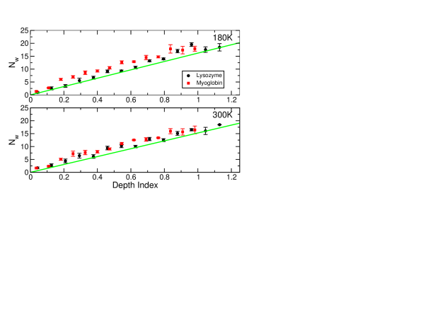
Figure 1: Number of water molecules as a function of the depth index at 180 K and 300 K for lysozyme and myoglobin. The straight lines are obtained from Eq. 2.

We compute the average number of water molecules both in the hydration shell of each residue and in the bulk. The bulk values are 32.4 and 30.5 water molecules at 180 K and 300 K, respectively, corresponding to a density of 1070 ${\rm kg/m}^{3}$ and 1007 ${\rm kg/m}^{3}$. The results are depicted in Fig. 1, and are in agreement with the linear dependence predicted by Eq. 2 for both proteins. Hence, the temperature dependence of the distribution of water molecules in the protein is determined predominantly from the bulk value $\rho(T)$. Local structural irregularities and protein dynamics have a relatively minor role.

Although the distribution of water molecules, an equilibrium property, is not affected by temperature, the dynamics of water around the protein depends strongly on $T$. We characterize the latter by their residence times, $\tau_{r}$, which is the average time a molecule takes to escape from a given region. To measure the residence times of water molecules in the hydration shells of all residues, we partition the 50 ns long trajectories into fifty 1 ns long pieces, and record the initial number of hydration shell water molecules in each region. We then compute the decrease in the number of these water molecules as a function of time by checking if they remain in the hydration shell. Since the trajectories are recorded in intervals of 0.4 ps, water molecules that cross the boundary and return to the monitored layer faster than that time scale are assumed to have remained. We depict in Fig. 2 this decrease for selected residues of lysozyme, a highly buried one CYS30 ($d=0.065$), one at an intermediate depth ASN65 ($d=0.435$), a surface residue THR47 ($d=1.26$) and finally the escape process in the bulk ($d=2$).

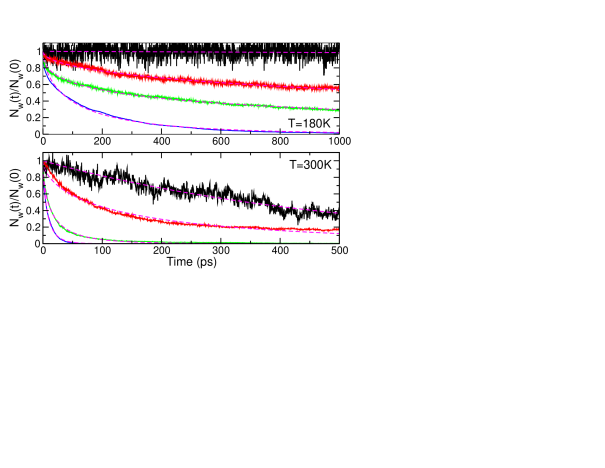
Figure 2: Normalized number of water molecules initially residing in the vicinity of a residue as a function of time. Samples are for residues with different depth indices (CYS30: $d=0.065$, ASN65: $d=0.435$, THR47: $d=1.26$) and in the bulk ($d=2$). The dashed lines represent the stretched exponential fits. $d$ increases from the top towards the bottom curves.

Many different processes contribute to the curves in Fig. 2. Most of the water molecules are close to the edge of the sphere we consider, and thus can escape faster on average. On the other hand, the water molecules at the center of the sphere initially will remain longer. There will also be additional contributions from the fluctuating chain molecule. Consequently, one expects to have a superposition of exponential decays for $N_{w}(t)$ which is best described by a stretched exponential function, Williams and Watts (1970)

$$N_{w}(t)=\langle N_{w}\rangle\;\exp{\left[-(t/\tau_{r})^{\beta}\right]},$$ (3)

where $\tau_{r}$ is the effective residence time and $\beta$ is the stretched exponent. The fits are illustrated in Fig. 2 and are in good agreement with the MD results, validating the model. The stretched exponent has a value $\beta\approx 0.5$ regardless of the location of the residue and temperature. We thus compute the residence times for all the residues of lysozyme and myoglobin, and plot them as a function of depth index in Fig. 3.

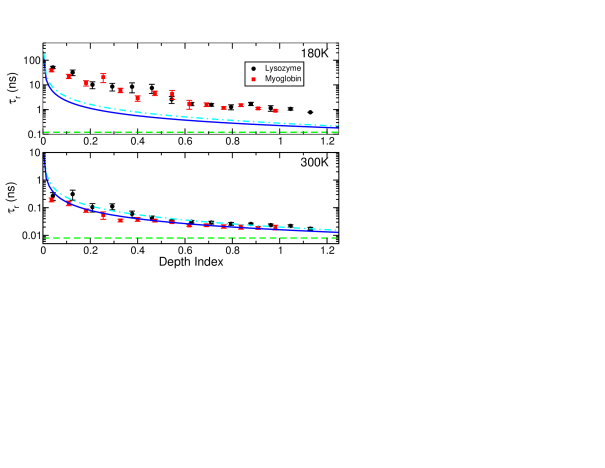
Figure 3: Residence times of water molecules as a function of the depth index for lysozyme and myoglobin from fits to Eq. 3. The stretched exponents fluctuate around 0.5 at all depths and temperatures for both proteins. The limiting value in the bulk is represented by the dashed lines. Predictions from Eq. 5 (solid line) and from Bezrukov el al. Bezrukov et al. (2001) (dot-dashed line) are also shown.

The residence times for equivalent depths can have important variations because of the residue specificities and their spatial arrangements. For example, residues can be hydrophobic or hydrophilic, and consequently decrease or increase the residence time of the surrounding water. Moreover, residues can be concentrated in one region of the hydration shell facilitating the escape process. However, one can capture the general trend when considering a large number of residues. Differences of up to three orders of magnitude between the residence times of solvent molecules buried in the protein compared to those near the surface are observed. This is due to the fact that the water molecules inside have to escape traps formed by the residues. Thus, the higher the coordination number of a residue, the larger the number of traps, and the longer the escape time. Note that, for certain residues that display extremely slow decay profiles at 180 K (exemplified by the uppermost curve in Fig. 2), Eq. 3 provides residence times longer than 100 ns. This is due to the error involved in extrapolation of the initial decay profiles to very long time scales.

Using a model of diffusive motion in the presence of local obstacles, a relationship may be derived for the residence time as a function of depth. As a first order approximation, we assume the probability to escape from the neighborhood of a residue $P_{r}$ decreases linearly with the occupied volume as

$$P_{r}=P_{0}\left(1-\frac{V_{r}}{V_{0}}\right)\;,$$ (4)

where $P_{0}$ is the probability of escaping in the bulk and $V_{r}=\sum_{j=1}^{N_{c}}V_{j}$ the occupied volume around the residue. The occupied volume is the total volume minus the available volume $V_{r}=V_{0}-V_{a}$; using $d=2V_{a}/V_{0}$ (Eq. 1), one gets $P_{r}=P_{0}\;d/2$. Since the residence time scales inversely with the probability of escape, Gaspard (1998) and the proportionality constant is assumed to be an intrinsic property of the escaping species irrespective of the local environment, one gets,

$$\tau_{r}(d)=\tau_{B}\;\frac{2}{d}\;.$$ (5)

where $\tau_{B}$ is the residence time in the bulk. In Fig. 3, we display the findings from Eq. 5 along with the results from the highly elaborate analytical solution of Bezrukov et al. Bezrukov et al. (2001) for the probability of diffusion displacement of a molecule using the fraction of possible trajectories in the presence of obstacles. The rather simple model of Eq. 5 captures the main features of this detailed analytical solution. We further find that both approaches predict the depth dependence at 300 K, while they fail to do so at 180 K.

So far as the predictions of Eq. 5 reproduce the main features of water behavior around the protein at room temperature, they corroborate that specificity plays a lesser role in determining residence times at physiological temperatures. Luise et al. (2000); Makarov et al. (2000) Below $T_{d}$, however, we find that the simple trapped diffusion idea does not capture the dynamics of water. In fact, the calculated residence times are approximately one order of magnitude slower than predicted by the theory, indicating that the dynamics is not controlled by diffusion in the presence of obstacles, hence suggesting that hydration shell water is not liquid below the transition temperature. This confirms the observation that translational diffusion is hindered below the dynamical transition. Tournier et al. (2003)

III.2 Depth dependent relaxation times in the hydration layer

To further investigate the water/protein interactions, we quantify the dynamics of the protein, hydration layer, and bulk solvent by measuring relaxation times. For the $C_{\alpha}$ atom of the ith residue, we follow the decay of the correlation function,

$$C^{\alpha}_{i}(t)=\frac{\langle\Delta\mathbf{R}_{i}(t)\cdot\Delta\mathbf{R}_{i}(0)\rangle}{\langle\Delta\mathbf{R}_{i}^{2}\rangle}$$ (6)

where $\Delta\mathbf{R}_{i}(t)=\mathbf{R}_{i}(t)-\langle\mathbf{R}_{i}\rangle$ is the fluctuation vector of the atom. We note that $\langle\mathbf{R}_{i}\rangle$ is computed for each 0.5 ns trajectory piece and then a best fit superposition is performed to separate the internal motion of the protein from long time tumbling. Previously, this method permitted evaluating the dynamical transition temperature for different protein-solvent systems. Baysal and Atilgan (2005); Atilgan et al. (2008)

Many different processes over a wide range of time scales contribute to the backbone dynamics as we recently discussed in detail. Okan et al. (2009) Here we employ stretched exponential functions on the correlation functions of Eq. 6 to fit the initial decay processes as in our previous work. Atilgan et al. (2008) We depict in Fig. 4 the correlation function for the three residues of lysozyme also exemplified in Fig. 2 and the corresponding stretched exponential fits. We note that the long time tails of these relaxation functions belong to more collective dynamics with a nanosecond time scale, which we do not further elaborate upon since this was discussed in great detail recently. Okan et al. (2009)

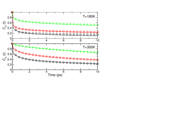
Figure 4: $C_{\alpha}$ correlation function for residues with different depth indices. The circles are for the buried residue (CYS30, $d=0.065$), the squares for the intermediate (ASN65, $d=0.435$) and the diamonds for the surface one (THR47, $d=1.26$). The straight lines represent the stretched exponential fits.

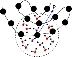
Figure 5: Schematic representation of the hydration shell of a residue and the local polarization vector $P$.

Closely associated with backbone dynamics, we further compute the water relaxation times by using the local polarization vector $\mathbf{P}_{i}$ in the vicinity of each $C_{\alpha}$ as depicted in Fig. 5. One can then compute the following correlation function,

$$C^{w}_{i}(t)=\frac{\langle\Delta P_{i}(t)\Delta P_{i}(0)\rangle}{\langle\Delta P_{i}^{2}\rangle}$$ (7)

where $\Delta P_{i}(t)=|\mathbf{P}_{i}(t)|-\langle|\mathbf{P}_{i}(t)|\rangle$ is the fluctuation of the norm of the polarization vector of the ith residue. The polarization vector is the sum of the polarization vectors of the water molecules within the hydration shell of the residue considered,

$$\mathbf{P}_{i}(t)=\sum_{j\in i}\mathbf{p}_{j}(t).$$ (8)

We emphasize that we use a difference definition utilizing the norms (7), as opposed to the usual expression involving the scalar product of the dipolar moments. While the dipolar moment in the bulk is equal to zero on average, it is not the case inside the protein, where water molecules can have preferred orientations because of the proximity of protein atoms. Consequently we use the quantity $\Delta P_{i}(t)$ which eliminates this bias, in addition to the advantage of Eq. (7) providing a faster decay since it corresponds to a higher moment. Moreover, we note that the relaxation time obtained depends on the number of water molecules considered for either definition of the relaxation.van der Spoel et al. (1998) To recover the experimental value of the relaxation time, one should compute the polarization vector for larger spheres. At room temperature, we find that the radius should be larger than the correlation length of the solvent which is ca. $12\;\AA$. Beyond this sphere size, the Debye relaxation time converges to the value of 7.3 $\pm$ 0.7 ps, as also reported in literature previously for TIP3P water model Höchtl et al. (1998), and compares well with the experimental value of 8.2 ps. In contrast, for the sphere size chosen in this work, $6\;\AA$, the value is 5 ps. For the relaxation function of Eq. (7), the respective relaxation times are 3.2 and 1.8 ps for spheres of radius $12\;\AA$ and $6\;\AA$, respectively. Thus, our computed values of the relaxations are consistent within this work, and are useful for comparing the local dynamics of water clusters at various depths. However, they cannot be compared directly with Debye relaxation times.

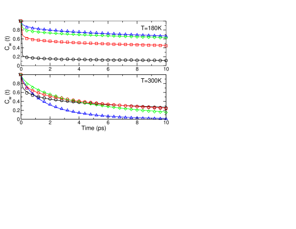
Figure 6: Local water polarization correlation function as a function of time for different depth indices. The straight lines represent the stretched exponential fits. Symbols are the same as in Fig. 4. Triangles are for bulk water.

As for the backbone, we use stretched exponential fits to the initial decay region of the correlation function to extract the relaxation times. We depict in Fig. 6, for the three typical residues and the bulk, the correlation functions along with the corresponding fits. We note that, here we study the dynamics of a group of water molecules, and not the dipolar relaxation of individual water molecules. The former permits us to study collectivity and hence evaluate the glassy behavior of water clusters around individual residues.

We observe that for both the backbone and the water molecules, the short time relaxation is relatively well described by the stretched exponential functions. For longer times a slower, single exponential decay also appears in the water correlation functions, attributed to the large scale reconfiguration of the water molecules inside the region. However, for the current purpose of studying water/backbone dynamics on the picosecond time scales, we focus our attention to the former relaxations of both the backbone and the hydration shell water.

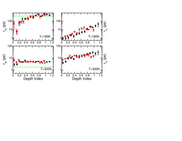
Figure 7: Relaxation times of $C_{\alpha}$ atoms and water molecules as a function of the depth index for lysozyme (circles) and myoglobin (squares). The straight lines indicate bulk water relaxation times.

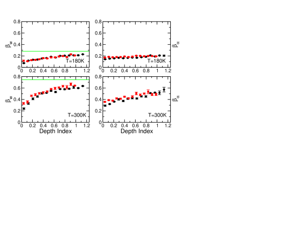
Figure 8: Stretched exponents of $C_{\alpha}$ atoms and water molecules as a function of the depth index for lysozyme (circles) and myoglobin (squares). The straight lines indicate bulk water values.

Having validated the model for the correlation functions, we compute the relaxation times for each residue of lysozyme and myoglobin. We depict them as a function of depth index in Fig. 7 and their corresponding stretched exponents in Fig. 8 for the two temperatures. We observe that the relaxation times of $C_{\alpha}$ atoms ($\tau_{\alpha}$) are higher at room temperature than at 180 K (the average values are 13 ps and 6 ps, respectively). We have previously explained this slowing down of the local relaxations using a model that relates the onset of the coupling between the local internal motions of the protein to the hydration layer with temperature. The results showed that such behavior is due to the interplay between the decreased stiffness and the modified effective friction coefficient. Atilgan et al. (2008) Moreover, independent of temperature, $\tau_{\alpha}$ increases with depth index, which may be explained by packing arguments: The more buried a residue is, the larger is the coordination number, and hence the local rigidity of the medium. Consequently, the magnitude of fluctuations is smaller, leading to faster relaxations.

Conversely, relaxations of water molecules forming the hydration shell ($\tau_{w}$) are observed to speed up with increasing temperature. At 180 K, their values are highly depth index dependent, accompanied by slowly increasing stretched exponents with values close to $\beta=0.2$. The latter is indicative of a collection of trapped states for the rotational motion of water molecules according to a model of hierarchically ordered materials. Frisch and Sornette (1997); Klafter and Shlesinger (1986); Metzler et al. (1999) Thus, the water layer shows a strong tendency to be affected by the local environment (i.e. packing) below $T_{d}$. However, their dynamics is independent of depth index at 300 K beyond a critical depth index ($d$ = 0.3), where there are at least five water molecules surrounding a given residue (see Fig. 1), marginally enough to form a polarized “water layer”. The relaxations have a characteristic time scale of approximately 5 ps at room temperature. The distribution of relaxation times is much narrower as indicated by the larger stretched exponents of $\beta>0.4$ (see Okan et al. Okan et al. (2009) for a detailed interpretation of stretched exponents).

The fact that $\tau_{w}$ are on the same order as $\tau_{\alpha}$ at 300 K, along with their depth independence suggests that water and overall protein dynamics are coupled at physiological temperatures, supporting the idea that water forms a vicinal layer around the protein, Atilgan et al. (2008) accompanied by a large water reorganization energy. LeBard and Matyushov (2008) In contrast, $\tau_{w}$ values are $1-2$ orders of magnitude slower than $\tau_{\alpha}$ at 180 K, along with a very strong dependence on the local environment.

Moreover, at room temperature hydration shell water relaxes slower than bulk water, compatible with a more viscous layer, slowed down by the interactions with the residues. On the other hand, below the transition, due to the lack of larger displacement within the hydration shell, hydration water relaxes faster than the bulk. This suggests that within the time scale of the observations leading to the correlation function, the hydration shell water is in a glassy state.

These findings corroborate the results on the residence times in Fig. 3. They lead to a better understanding of the relationship between water-protein interactions and the dynamical transition. We further investigate this by computing the relaxation times of the motions described by Eq. 7 for lysozyme over a wide temperature range.

III.3 Gradual unfreezing of the hydration layer

We have produced 24 ns trajectories for lysozyme at 13 separate temperatures spanning 160 to 300 K and computed the relaxation times of the hydration shell and bulk water. We observed in Fig. 7 that below $T_{d}$, hydration shell water relaxes faster than the bulk if the residue’s location is deep enough. To observe the transition from faster to slower relaxation, or in other words from glassy to liquid, one can simply count the number of residues slower than the bulk at each temperature as depicted in Fig. 9.

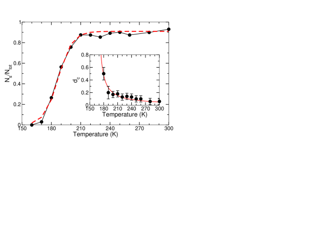
Figure 9: Normalized number of residue for which the hydration shell relaxation time is slower than that of bulk water. The dashed line represents a Boltzmann sigmoid fit yielding a midpoint value at 187 K. The inset represents the critical depth index $d_{c}$ as a function of temperature, the line is a guide for the eye.

One can then measure the critical depth index $d_{C}$ beyond which the hydration shell water becomes slower than the bulk, as shown in the inset to Fig. 9. We observe a marked transition from a state where all the hydration shell waters are faster than the bulk to the opposite. The observed behavior may be described by a gradual unfreezing of the hydration shell. At temperatures just above $T_{g}$ of water (see the Appendix for a prediction of the $T_{g}$ of the TIP3P water model in the range of 150 - 160 K), only the outermost hydration shells are not frozen. For example at 180 K, residues of depth index approximately larger than 0.5 have equivalent relaxation times to bulk water (also see Fig. 7). We note that some water molecules ($\sim$10$\%$) remain faster than the bulk even at temperature well-above $T_{d}$; these are highly buried water molecules that remain coupled to the protein. The gradual unfreezing of the hydration shell enhances our understanding of the dynamical transition occurring within a wide time and temperature range, determined by the time scale of solvent coupled structural relaxations. It has already been suggested that the broadening in the glass transition of the protein hydration shell is due to a distribution of water clusters with different glass transition temperatures. Doster et al. (1986) The heterogeneity of the hydration shell quantified by the depth index and its relation to the hydration levels, residence times and relaxation times expands on this view.

IV CONCLUSION

We study the residence times and memory loss of water molecules around individual residues to interpret their role in the dynamics of folded proteins. The calculations are repeated for two well-studied proteins, leading to identical results: Above $T_{d}$ the residence time of water molecules around a given residue may be interpreted via a simple depth dependent model of trapped diffusion. The memory loss of the polarization vector displays a similar trend to that of the protein backbone in terms of the time scales involved. Okan et al. (2009) In contrast, the dynamics of water molecules are non-diffusive in the regime below $T_{d}$. Consequently, below $T_{d}$ the hydration shell is solid-like, behaving as a crust around the protein. Upon heating, the hydration shell is unfrozen, and permits the transfer of entropy from the bulk to the protein by the entry/exit process of water molecules, hence acting as a plasticizer and increasing the overall flexibility of the protein. The contrast between the water dynamics in the hydration shell of a protein at physiological and non-physiological temperatures therefore reveals the interactions and the free energetic requirements necessary to achieve biologically relevant motions.

Bulk and hydration layer water have been shown to separately control motions in functional proteins; for example, the former allows ligand entry/exit, while the latter is responsible for migration of ligands within the protein. Frauenfelder et al. (2009) The hydration layer acts as a lubricant for the onset of the functional dynamics in the protein, as new channels between conformational substates emerge, e.g. through jumps enabled in the side-chain torsional angles. Markelz et al. (2007) Our results demonstrate that hydration water not only performs localized motions, but also participates in the global dynamics through long-range diffusion. Below the transition temperature, on the other hand, the miscommunication between the substates maintains the trapped hydration water highly dependent on the dynamics of the protein.

V APPENDIX

V.1 Glass transition temperature of TIP3P water

One of the crucial quantities regarding the dynamical transition in proteins is the water glass transition temperature. The glass transition temperature is defined as the temperature at which the shear viscosity is $10^{12}\;{\rm Pa.s}$, corresponding to a relaxation time of approximately 100 s. It is also marked by a crossover from ergodic to non-ergodic behavior. Experimentally, a step-like decrease in the susceptibilities (e.g. heat capacity) is observed. It was suggested that the dynamical transition of the protein is dictated by the glass transition of the solvent. Ansari et al. (1987); Wong et al. (1989); Vitkup et al. (2000b) Although pure water readily forms the ice-phase and is very difficult to vitrify, an experimental value of $\sim 165$ K has nevertheless been measured. Velikov et al. (2001); Yue and Angell (2004) To evaluate the influence of glassy water on the protein, we must first assess the behavior of the water model used in this study.

The specific heat may be computed from

$$C=\frac{\langle E^{2}\rangle-\langle E\rangle^{2}}{k_{B}T^{2}},$$ (9)

and the isothermal compressibility as

$$\kappa_{T}=\frac{\langle V^{2}\rangle-\langle V\rangle^{2}}{k_{B}T\langle V\rangle}\;,$$ (10)

where $E$ is the total energy of the system and $V$ the volume. The results along with experimental values are depicted in Fig. 10. The specific heat and compressibility curves yield a glass transition temperature between 150 K and 160 K. This value is lower than the SPC/E, TIP4P and TIP5P water models, Brovchenko et al. (2005) though closer to the experimental value, Velikov et al. (2001); Yue and Angell (2004) in accordance with the fact that TIP3P water is less structured than the other water models. Tan et al. (2003)

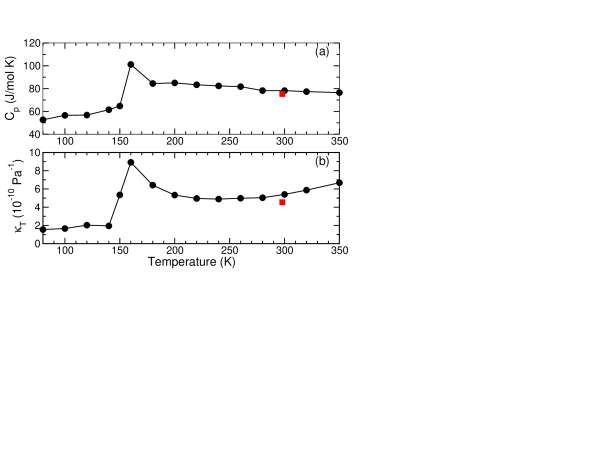
Figure 10: Temperature dependence of the (a) isobaric specific heat, (b) isothermal compressibility. The squares represent the experimental values at room temperature. Tipler (1999); Halliday et al. (1997)

One may also predict the transition by computing the shear viscosity $\eta$. In equilibrium, one can evaluate $\eta$ either from the mean square displacement of the Helfand moment associated to viscosity,Viscardy et al. (2007) or from the Green-Kubo relation,

$$\eta=\frac{V}{k_{B}T}\int_{0}^{\infty}dt\;\langle P_{\alpha\beta}(t)P_{\alpha\beta}(0)\rangle,$$ (11)

where $V$ is the volume of the system, $T$ the temperature, $k_{B}$ the Boltzmann constant, and $P_{\alpha\beta}$ the pressure tensor,

$$P_{\alpha\beta}=\frac{1}{V}\left(\sum_{i}m_{i}v_{i}^{\alpha}v_{i}^{\beta}+\sum_{i<j}F_{ij}^{\alpha}r_{ij}^{\beta}\right).$$ (12)

where $\alpha$ and $\beta$ take the values $x$,$y$ and $z$. The off-diagonal components of $P_{\alpha\beta}$ permit to compute the shear viscosity $\eta$ while the diagonal ones lead to the bulk viscosity. Note that the value of the viscosity calculated by Eq. 11 is limited by the length of the simulations.

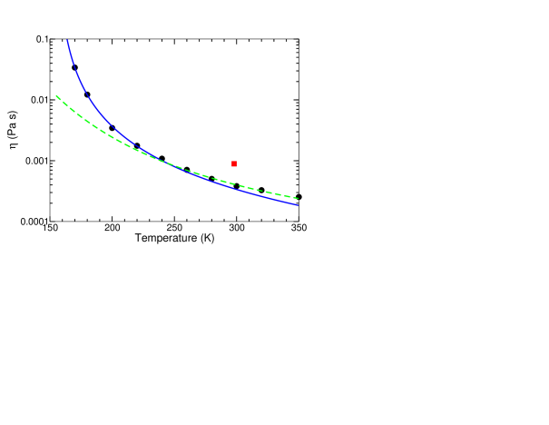
Figure 11: Temperature dependence of the shear viscosity $\eta$. The square represent the experimental value at room temperature. Franks (2000) The plain line is the result of the power law fit at low temperatures and yields $T_{g}=155$ K and $\gamma=2.1$. The dashed line is the Arrhenius behavior for high temperatures.

One can then estimate the glass transition temperature $T_{g}$ by fitting the power law $\eta\sim|T-T_{g}|^{-\gamma}$. We depict in Fig. 11 the temperature dependence of the shear viscosity and the power law fit. The fit yields a glass transition temperature $T_{g}=155$ K in accord with the values obtained from the susceptibilities.

References

- Doster et al. (1989) W. Doster, S. Cusack, and W. Petry, Nature 337, 754 (1989).
- Doster (2008) W. Doster, Eur. Biophys. J. 37, 591 (2008).
- Doster et al. (2010) W. Doster, S. Busch, A. M. Gaspar, M.-S. Appavou, J. Wuttke, and H. Scheer, Phys. Rev. Lett. 104, 098101 (2010).
- Doster (2010) W. Doster, BBA, Proteins and Proteomics 1804, 3 (2010).
- Atilgan et al. (2008) C. Atilgan, A. O. Aykut, and A. R. Atilgan, Biophys. J 94, 79 (2008).
- Tsai et al. (2001) A. M. Tsai, T. J. Udovic, and D. A. Neumann, Biophys. J. 81, 2339 (2001).
- Steinbach and Brooks (1996) P. J. Steinbach and B. R. Brooks, Proc. Natl. Acad. Sci. USA 93, 55 (1996).
- Yu et al. (2003) X. Yu, J. Park, and D. M. Leitner, J. Phys. Chem. B 107, 12820 (2003).
- Doster and Settles (2005) W. Doster and M. Settles, Biochim Biophys Acta 1749, 173 (2005).
- Zhang et al. (2007) L. Zhang, L. Wang, Y.-T. Kao, W. Qiu, Y. Yang, O. Okobiah, and D. Zhong, Proc. Natl. Acad. Sci. USA 104, 18461 (2007).
- Arcangeli et al. (1998) C. Arcangeli, A. R. Bizzarri, and S. Cannistraro, Chem. Phys. Lett. 291, 7 (1998).
- Vitkup et al. (2000a) D. Vitkup, D. Ringe, G. A. Petsko, and M. Karplus, Nature Struct. Biol. 7, 34 (2000a).
- Tarek and Tobias (2002) M. Tarek and D. J. Tobias, Phys. Rev. Lett. 88, 138101 (2002).
- Kumar et al. (2006) P. Kumar, Z. Yan, L. Xu, M. G. Mazza, S. V. Buldyrev, S.-H. Chen, S. Sastry, and H. E. Stanley, Phys. Rev. Lett. 97, 177802 (2006).
- Qvist et al. (2009) J. Qvist, E. Persson, and C. Halle, Faraday Discuss. 141, 131 (2009).
- Phillips et al. (2005) J. C. Phillips, R. Braun, W. Wang, J. Gumbart, E. Tajkhorshid, E. Villa, C. Chipot, R. D. Skeel, L. Kale, and K. Schulten, J. Comput. Chem. 26, 1781 (2005).
- Brooks et al. (1983) B. R. Brooks, R. E. Bruccoleri, B. D. Olafson, D. J. States, S. Swaminathan, and M. Karplus, J. Comput. Chem. 4, 187 (1983).
- Okan et al. (2009) O. Okan, A. Atilgan, and C. Atilgan, Biophys. J. 97, 2080 (2009).
- Makarov et al. (1998) V. A. Makarov, M. Feig, B. K. Andrews, and B. M. Pettitt, Biophys. J. 75, 150 (1998).
- Ebbinghaus et al. (2007) S. Ebbinghaus, S. J. Kim, M. Heyden, X. Yu, U. Heugen, M. Gruebele, D. M. Leitner, and M. Havenith, Proc. Natl. Acad. Sci. USA 104, 20749 (2007).
- Varrazzo et al. (2005) D. Varrazzo, A. Bernini, O. Spiga, A. Ciutti, S. Chiellini, V. Venditti, L. Bracci, and N. Niccolai, Bioinformatics 21, 2856 (2005).
- Merzel and Smith (2002) F. Merzel and J. C. Smith, Proc. Natl. Acad. Sci. USA 99, 5378–5383 (2002).
- Williams and Watts (1970) G. Williams and D. C. Watts, Trans. Faraday Soc. 66, 80 (1970).
- Gaspard (1998) P. Gaspard, Chaos, Scattering, and Statistical Mechanics (Cambridge University Press, Cambridge, 1998).
- Bezrukov et al. (2001) O. F. Bezrukov, A. E. Lukyanov, V. K. Pozdyshev, and A. V. Struts, Physica Scripta. 64, 382 (2001).
- Luise et al. (2000) A. Luise, M. Falconi, and A. Desideri, Proteins 39, 56 (2000).
- Makarov et al. (2000) V. A. Makarov, B. K. Andrews, P. E. Smith, and B. M. Pettitt, Biophys. J. 79, 2966 (2000).
- Tournier et al. (2003) A. Tournier, J. Xu, and J. Smith, Biophys. J. 85, 1871 (2003).
- Baysal and Atilgan (2005) C. Baysal and A. R. Atilgan, Biophys. J. 88, 1570 (2005).
- van der Spoel et al. (1998) D. van der Spoel, P. J. van Maaren, and H. J. C. Berendsen, J. Chem. Phys. 108, 10220 (1998).
- Höchtl et al. (1998) P. Höchtl, S. Boresch, W. Bitomsky, and O. Steinhauser, J. Chem. Phys. 109, 4927 (1998).
- Frisch and Sornette (1997) U. Frisch and D. Sornette, J. Phys. I. 7, 1155 (1997).
- Klafter and Shlesinger (1986) J. Klafter and M. F. Shlesinger, Proc. Natl. Acad. Sci. USA 83, 848 (1986).
- Metzler et al. (1999) R. Metzler, J. Klafter, and J. Jortner, Proc. Natl. Acad. Sci. USA 96, 11085 (1999).
- LeBard and Matyushov (2008) D. N. LeBard and D. V. Matyushov, Phys. Rev. E 78, 061901 (2008).
- Doster et al. (1986) W. Doster, A. Bachleitner, R. Dunau, M. Hiebl, and E. Lüscher, Biophys. J. 50, 213 (1986).
- Frauenfelder et al. (2009) H. Frauenfelder, G. Chen, J. Berendzen, P. W. Fenimore, H. Jansson, B. H. McMahon, I. R. Stroe, J. Swenson, and R. D. Young, Proc. Natl. Acad. Sci. USA 106, 5129 (2009).
- Markelz et al. (2007) A. G. Markelz, J. R. Knab, J. Y. Chen, and Y. He, Chem. Phys. Lett. 442, 413 (2007).
- Ansari et al. (1987) A. Ansari, J. Berendzen, D. Braunstein, B. R. Cowen, H. Frauenfelder, M. K. Hong, I. E. Iben, J. Johnson, P. Ormos, T. B. Sauke, et al., Biophys. Chem 26, 337 (1987).
- Wong et al. (1989) C. F. Wong, C. Zheng, and J. A. McCammon, Chem. Phys. Lett. 154, 151 (1989).
- Vitkup et al. (2000b) D. Vitkup, D. Ringe, G. A. Petsko, and M. Karplus, Nat. Struct. Biol. 7, 34 (2000b).
- Velikov et al. (2001) V. Velikov, S. Borick, and C. A. Angell, Science 294, 2335 (2001).
- Yue and Angell (2004) Y. Yue and C. A. Angell, Nature 427, 717 (2004).
- Brovchenko et al. (2005) I. Brovchenko, A. Geiger, and A. Oleinikova, J. Chem. Phys. 123, 044515 (2005).
- Tan et al. (2003) M.-L. Tan, J. T. Fischer, A. Chandra, B. R. Brooks, and T. Ichiye, Chemical Physics Letters 376, 646 (2003).
- Viscardy et al. (2007) S. Viscardy, J. Servantie, and P. Gaspard, J. Chem. Phys. 126, 184512 (2007).
- Franks (2000) F. Franks, Water, A Matrix of Life 2nd Ed. (The Royal Society of Chemistry, London, 2000).
- Tipler (1999) P. A. Tipler, Physics for Scientists and Engineers 4th Ed. (W. H. Freeman, London, 1999).
- Halliday et al. (1997) D. Halliday, R. Resnick, and J. Walker, Fundamentals of Physics 5th Ed. (Wiley, New York, 1997).