A New Technique for Determining Europium Abundances in Solar-Metallicity Stars

Abstract

We present a new technique for measuring the abundance of europium, a representative r-process element, in solar-metallicity stars. Our algorithm compares LTE synthetic spectra with high-resolution observational spectra using a $\chi^{2}$-minimization routine. The analysis is fully automated, and therefore allows consistent measurement of blended lines even across very large stellar samples. We compare our results with literature europium abundance measurements and find them to be consistent; we also find our method generates smaller errors.

1. Introduction

Every atom heavier than lithium has been processed by stars. Elements of the $\alpha$ process, iron peak, and r process have different formation sites, and therefore, understanding the distribution of these elements in nearby stars can lead to a better understanding of the Galaxy’s chemical enrichment history. The r-process site is the least well understood. Europium is our choice for an r-process investigation for two reasons: 96% of Galactic europium is formed through the r-process (Burris et al., 2000), and it has several strong lines in the visible portion of the electromagnetic spectrum. In order to provide insight into the Galactic enrichment history, however, europium measurements in very large stellar samples will be needed.

The study of r-process elements is well established in metal-poor stars (e.g., Sneden et al., 2008; Lai et al., 2008; Frebel et al., 2007; Simmerer et al., 2004; Johnson & Bolte, 2001), where r-process abundances probe early Galactic history. A handful of studies have measured europium in solar-metallicity stars (e.g., Reddy et al., 2006; Bensby et al., 2005; Koch & Edvardsson, 2002; Woolf et al., 1995), but have done so in samples of 50–200 stars. We aim to extend such work to a substantial sample of 1000 stars at solar metallicity, using spectra collected by the California and Caltech Planet Search (CCPS). Such a large sample will require automated analysis.

Our goal in this paper is to establish a new, automated abundance fitting method based on Spectroscopy Made Easy (SME; Valenti & Piskunov, 1996), an LTE spectral synthesis code discussed in further detail in § 3. The analysis builds on the framework of the Valenti & Fischer 2005 (hereafter VF05) Spectroscopic Properties of Cool Stars (SPOCS) catalog. Our method will yield consistent results across large stellar samples, generating smaller errors than previous analyses.

We begin here with 41 stars that have been examined in the literature, and we include three europium lines: 4129 Å, 4205 Å, and 6645 Å. Our stellar observations are detailed in § 2. We describe the details of our europium abundance measurement algorithm in § 3, compare our values with existing europium literature in § 4, and summarize the results of the study in § 5.

2. Observations

The spectra of the 41 stars included in this study were taken with the HIRES echelle spectrograph (Vogt et al., 1994) on the 10-m Keck I telescope in Hawaii. The spectra date from January 2004 to September 2008 and have resolution $R\sim 50\,000$ and signal-to-noise ratio (S/N) of $\sim$ $160$ near 4200 Å, where the two strongest Eu ii lines included in this study are located. The spectra have the same resolution but S/N $\sim 340$ at 6645 Å, where a third, weaker Eu ii line is located.

The spectra were originally obtained by the CCPS with the intention of detecting exoplanets. The CCPS uses the same spectrometer alignment each night and employs the HIRES exposure meter (Kibrick et al., 2006), so the stellar observations are extremely consistent, even across years of data collection. For a more complete description of the CCPS and its goals, see Marcy et al. 2008. It should be noted that the iodine cell Doppler technique (Marcy & Butler, 1992) imprints molecular iodine lines only between the wavelengths of 5000 and 6400 Å, leaving the regions of interest for this study iodine free.

2.1. Stellar Sample

For this study we choose to focus on a subset of stars that have been analyzed in other abundance studies. We compare our measurements with those from Woolf et al. 1995; Simmerer et al. 2004; Bensby et al. 2005; and del Peloso et al. 2005. We select CCPS target stars that have temperature, gravity, mass, and metallicity measurements in the SPOCS catalog (VF05).

Our initial stellar sample consisted of 44 objects that were members both of the aforementioned studies and the SPOCS catalog, and that were observed by the CCPS on the Keck I telescope. Three stars that otherwise fit our criteria, but for which we could only measure the europium abundance in one line, were removed from the sample. They were HD 64090, HD 188510, and HIP 89215. While stellar europium abundances may be successfully measured from a single line, the goal of this study is to establish the robustness of our method, and so we deem it necessary to determine the europium abundance in at least two lines to include a star in our analysis here. We describe our criteria for rejecting a fit in § 3.2.

The 41 stars included in this study have $3.4<V<10.0$, $0.50<B-V<0.92$, and $5<d<75\textrm{ pc}$ (Hipparcos; ESA 1997). VF05 determine stellar properties using SME, so it is reasonable to adopt their values for our SME europium analysis. Based on the VF05 analysis, our stars have metallicity $-1.4<\textrm{[M/H]}<0.4$, effective temperature $4940<T_{\rm eff}<6230$, and gravity $3.8<\log{g}<4.8$. It should be noted that throughout this study we use the [M/H] parameter for a star’s metallicity, rather than the iron abundance [Fe/H]. Our [M/H] value is taken from VF05, where it is an independent model parameter that adjusts the relative abundance of all metals together. It is not an average of individual metal abundances. The full list of stellar properties, from the Hipparcos and SPOCS catalogs, appears in Table 1.

Table 1Stellar Data.

Identification			$V$	$B-V$	$d$	$T_{\rm eff}$	[M/H]	$\log{g}$	Ref.
HD	HR	HIP	(mag)	(mag)	(pc)	(K)		(cgs)
3795	173	3185	6.14	0.72	28.6	5369	$-0.41$	4.16	1
4614	219	3821	3.46	0.59	6.0	5941	$-0.17$	4.44	4
6734	…	5315	6.44	0.85	46.4	5067	$-0.28$	3.81	1
9562	448	7276	5.75	0.64	29.7	5939	$0.19$	4.13	1, 2, 4
9826	458	7513	4.10	0.54	13.5	6213	$0.12$	4.25	4
14412	683	10798	6.33	0.72	12.7	5374	$-0.45$	4.69	1
15335	720	11548	5.89	0.59	30.8	5891	$-0.20$	4.07	4
16397	…	12306	7.36	0.58	35.9	5788	$-0.35$	4.50	1
22879	…	17147	6.68	0.55	24.3	5688	$-0.76$	4.41	1, 2, 4
23249	1136	17378	3.52	0.92	9.0	5095	$0.03$	3.98	1
23439	…	17666	7.67	0.80	24.5	5070	$-0.73$	4.71	3
30649	…	22596	6.94	0.59	29.9	5778	$-0.33$	4.44	4
34411	1729	24813	4.69	0.63	12.6	5911	$0.09$	4.37	4
43947	…	30067	6.61	0.56	27.5	5933	$-0.28$	4.37	2
45184	2318	30503	6.37	0.63	22.0	5810	$0.03$	4.37	1
48938	2493	32322	6.43	0.55	26.6	5937	$-0.39$	4.31	4
84737	3881	48113	5.08	0.62	18.4	5960	$0.14$	4.24	4
86728	3951	49081	5.37	0.68	14.9	5700	$0.11$	4.29	4
102365	4523	57443	4.89	0.66	9.2	5630	$-0.26$	4.57	2
…	…	57450	9.91	0.58	73.5	5272	$-1.42$	4.30	3
103095	4550	57939	6.42	0.75	9.2	4950	$-1.16$	4.65	3
109358	4785	61317	4.24	0.59	8.4	5930	$-0.10$	4.44	4
115617	5019	64924	4.74	0.71	8.5	5571	$0.09$	4.47	4
131117	5542	72772	6.30	0.61	40.0	5973	$0.10$	4.06	2
144585	…	78955	6.32	0.66	28.9	5854	$0.25$	4.33	1
156365	…	84636	6.59	0.65	47.2	5856	$0.24$	4.09	1
157214	6458	84862	5.38	0.62	14.4	5697	$-0.15$	4.50	4
157347	6465	85042	6.28	0.68	19.5	5714	$0.03$	4.50	1
166435	…	88945	6.84	0.63	25.2	5843	$0.01$	4.44	1
169830	6907	90485	5.90	0.52	36.3	6221	$0.08$	4.06	1
172051	6998	91438	5.85	0.67	13.0	5564	$-0.24$	4.50	1
176377	…	93185	6.80	0.61	23.4	5788	$-0.23$	4.40	1
179949	7291	94645	6.25	0.55	27.0	6168	$0.11$	4.34	1
182572	7373	95447	5.17	0.76	15.1	5656	$0.36$	4.32	1
190360	7670	98767	5.73	0.75	15.9	5552	$0.19$	4.38	1
193901	…	100568	8.65	0.55	43.7	5408	$-1.19$	4.14	3
199960	8041	103682	6.21	0.64	26.5	5962	$0.24$	4.31	1
210277	…	109378	6.54	0.77	21.3	5555	$0.20$	4.49	1
217107	8734	113421	6.17	0.74	19.7	5704	$0.27$	4.54	1
222368	8969	116771	4.13	0.51	13.8	6204	$-0.08$	4.18	4
224383	…	118115	7.89	0.64	47.7	5754	$-0.06$	4.31	1

2.2. Co-adding Data

The nature of the radial velocity planet search dictates that most stars will have multiple, and in some cases, dozens of, observations. To take advantage of the multiple exposures, we carefully co-add the reduced echelle spectra where possible.

The co-adding procedure is as follows: a 2000-pixel region (approximately half the full order width) near the middle of each order is cross-correlated, order by order, with one observation arbitrarily designated as standard. The pixel shifts are then examined and a linear trend as a function of order number is fit to the pixel shifts. For any order whose pixel shift falls more than 0.4 pixels from the linear trend, the value predicted by the linear trend is substituted. This method corrects outlying pixel shift values, which often proved to be one of a handful of problematic orders where the echelle blaze function shape created a false cross-correlation peak.

Each spectral order is adjusted by its appropriate fractional pixel shift before all the newly aligned spectra are added together. In order to accurately add spectra that have been shifted by non-integer pixel amounts, we use a linear interpolation between pixel values to artificially (and temporarily) increase the sampling density by a factor of 20. After the co-adding, the resultant high-S/N multi-observation spectrum is sampled back down to its original spacing.

The number of observations used per star is recorded in the $N_{obs}$ column of Table 2. The co-adding proved particularly beneficial when fitting the relatively weak Eu ii line at 6645 Å. Two sample stellar spectra, from a star with 1 observation and from a star with 17 observations, are given in Figure 1 as evidence of the S/N advantages of this procedure.

Table 2Stellar abundance values.

Name	$N_{obs}$	4129 Å	4205 Å	6645 Å	Weighted
		[Eu/H]	[Eu/H]	[Eu/H]	Average
3795	2	$0.07$	$0.06$	$0.13$	$0.07\pm 0.03$
4614	2	$-0.17$	$-0.19$	$-0.24$	$-0.18\pm 0.02$
6734	6	$-0.02$	$-0.06$	$0.01$	$-0.03\pm 0.03$
9562	3	$0.11$	$0.14$	$0.08$	$0.12\pm 0.02$
9826	1	$0.10$	$0.13$	$0.09$	$0.12\pm 0.02$
14412	70	$-0.28$	$-0.15$	$-0.16$	$-0.24\pm 0.06$
15335	2	$-0.13$	$-0.10$	$-0.08$	$-0.12\pm 0.03$
16397	1	$-0.21$	$-0.20$	$-0.22$	$-0.21\pm 0.02$
22879	27	$-0.55$	$-0.50$	$-0.57$	$-0.54\pm 0.03$
23249	34	$0.05$	$0.26$	$0.24$	$0.17\pm 0.11$
23439	24	$-0.43$	$-0.36$	$-0.47$	$-0.38\pm 0.03$
30649	3	$-0.13$	$-0.11$	$-0.13$	$-0.12\pm 0.02$
34411	70	$0.12$	$0.13$	$0.11$	$0.13\pm 0.02$
43947	6	$-0.21$	$-0.19$	$-0.21$	$-0.20\pm 0.02$
45184	95	$0.01$	$-0.03$	$0.02$	$0.00\pm 0.02$
48938	2	$-0.30$	$-0.28$	$-0.41$	$-0.30\pm 0.03$
84737	7	$0.14$	$0.14$	$0.14$	$0.14\pm 0.02$
86728	46	$0.06$	$0.11$	$0.10$	$0.09\pm 0.03$
102365	12	$-0.13$	$-0.08$	$-0.14$	$-0.11\pm 0.03$
HIP57450	1	$-1.10$	$-1.03$	$\leq-0.95$	$-1.06\pm 0.04$
103095	9	…	$-0.37$	$-0.38$	$-0.37\pm 0.02$
109358	47	$-0.12$	$-0.16$	$-0.12$	$-0.14\pm 0.03$
115617	165	$0.05$	$0.02$	$0.09$	$0.04\pm 0.03$
131117	2	$0.10$	$0.09$	$0.12$	$0.10\pm 0.02$
144585	17	$0.22$	$0.25$	$0.22$	$0.23\pm 0.03$
156365	1	$0.11$	$0.20$	$0.14$	$0.13\pm 0.04$
157214	24	$0.05$	$0.06$	$0.07$	$0.06\pm 0.02$
157347	77	$0.09$	$0.12$	$0.13$	$0.10\pm 0.02$
166435	1	$-0.05$	$-0.17$	$0.04$	$-0.07\pm 0.06$
169830	8	$0.02$	$0.05$	$0.05$	$0.03\pm 0.02$
172051	37	$-0.19$	$-0.15$	$-0.12$	$-0.17\pm 0.03$
176377	56	$-0.20$	$-0.21$	$-0.23$	$-0.20\pm 0.02$
179949	1	$0.05$	$0.02$	$0.05$	$0.04\pm 0.03$
182572	56	$0.25$	$0.41$	$0.36$	$0.31\pm 0.08$
190360	73	$0.17$	$0.29$	$0.30$	$0.24\pm 0.07$
193901	2	$-0.92$	$-0.91$	$-0.98$	$-0.91\pm 0.02$
199960	3	$0.14$	$0.19$	$0.19$	$0.16\pm 0.03$
210277	74	$0.20$	$0.34$	$0.32$	$0.27\pm 0.07$
217107	37	$0.20$	$0.43$	$0.33$	$0.29\pm 0.11$
222368	2	$0.08$	$0.09$	$0.08$	$0.08\pm 0.02$
224383	2	$0.00$	$-0.01$	$0.04$	$0.00\pm 0.02$
Vesta	3	$-0.04$	$0.00$	$0.00$	$-0.03\pm 0.03$

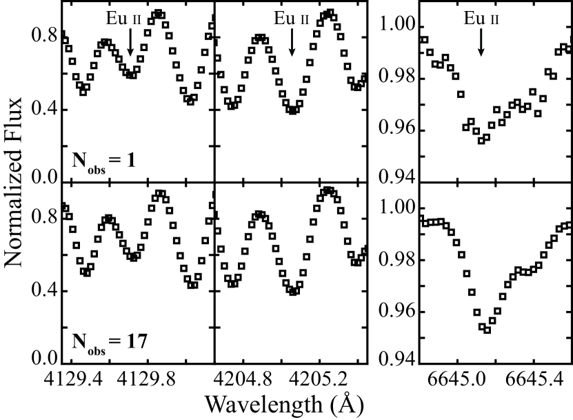
Figure 1.— The three Eu ii lines considered in this paper, plotted for two different stars to demonstrate the advantage to be gained from co-adding multiple observations of the same star. Note that the rightmost plots have a different ordinate axis scaling than the other four panels. The top three panels, showing HD 156365, include 1 spectrum, while the bottom three panels, showing HD 144585, include 17. The two stars have approximately the same metallicity and effective temperature. The advantage from co-adding is most profound in the weak 6645-Å line.

3. Abundance Measurements

We use the SME suite of routines for our spectral synthesis, both for fine-tuning line lists based on the solar spectrum (§ 3.1) and for measuring europium in each star (§ 3.2). SME is an LTE spectral synthesis code based on the Kurucz 1992 grid of stellar atmosphere models. In brief, to produce a synthetic spectrum, SME interpolates between the atmosphere models, calculates the continuous opacity, computes the radiative transfer, and then applies line broadening, which is governed by macroturbulence, stellar rotation, and instrumental profile. Consult Valenti & Piskunov 1996 and VF05 for a more in-depth description of SME’s inner workings.

Throughout this study we use SME only to compute synthetic spectra. All fitting is done in specialized routines of our own design, external to SME.

In this section we outline our technique for measuring europium abundances in the set of 41 stars included in this work. In broad strokes, we first determine the atomic parameters of our spectral lines by fitting the solar spectrum (§ 3.1). Then, we use that line list to measure the europium abundance in three transitions (4129 Å, 4205 Å, and 6645 Å); a weighted average of the three transitions determines a star’s final europium value (§ 3.2). Finally, we estimate our uncertainties by adding artificial noise to our data in a series of Monte Carlo trials (§ 3.3). We also here include notes on individual lines (§ 3.4).

3.1. Line Lists

We use relatively broad spectral segments in our europium analysis. The regions centered on the Eu ii 4129 Å and 6645 Å lines are 5 Å wide, and the region centered on the Eu ii 4205 Å line is 8 Å wide. We find it necessary to use such broad spectral segments in order to fit a robust and consistent continuum in the crowded blue regions.

Line lists are initially drawn from the Vienna Astrophysics Line Database (VALD; Piskunov et al. 1995; Kupka et al. 1999). The VALD line lists, in the regions surrounding all three Eu ii transitions, make extensive use of Kurucz line lists.

We apply the original VALD line list to an observed solar spectrum in order to determine the list’s completeness and to adjust line parameters as needed. In the blue, we use the disk-center solar spectrum from Wallace et al. 1998 with the following global parameters: $T_{\rm eff}$ $=5770\textrm{ K}$, $\log{g}=4.44$, [M/H] $=0$, microturbulence $v_{mic}=1.0\textrm{ km s${}^{-1}$}$, macroturbulence $v_{mac}=3.6\textrm{ km s${}^{-1}$}$, rotational velocity $v\sin{i}=0\textrm{ km s${}^{-1}$}$, and radial velocity $v_{rad}=0\textrm{ km s${}^{-1}$}$. These are the same solar parameters adopted in VF05. In the red, we find the Wallace et al. 1998 solar atlas to have insufficient S/N to accurately determine the atomic parameters. At 6645 Å, therefore, we instead compare our line list to the disk-integrated NSO solar spectrum (Kurucz et al., 1984), adjusting $v\sin{i}$ to $1.6\textrm{ km s${}^{-1}$}$ because the full solar disk has more substantial rotational broadening.

We find that adjustments to the oscillator strength ($\log{\textrm{\em gf}}$) and van der Waals broadening ($\Gamma_{6}$) parameters are required for the strongest lines in a given wavelength segment, even far from the Eu ii line of interest. For example, the Fe i line at 4202 Å has an equivalent width $W=326\textrm{ m\AA}$ in the Sun and significantly affects the continuum of the 4205-Å region. The $\log{\textrm{\em gf}}$ parameter controls the line depth while the $\Gamma_{6}$ parameter controls the line shape, so in general the two parameters are orthogonal.

We used the Kurucz $\log{\textrm{\em gf}}$ values provided by VALD where possible, but adjustments were necessary where line depths were poorly fit. For $\Gamma_{6}$, VALD returns the Barklem et al. 2000 parameters for beryllium through barium ($Z$ of 4–56), but has no $\Gamma_{6}$ values above $Z=56$. We therefore find it necessary to fit $\Gamma_{6}$ in species heavier than barium and in deep features not fit well by VALD values. We take particular care to determine the appropriate $\log{\textrm{\em gf}}$ and $\Gamma_{6}$ parameters for all lines adjacent to the Eu ii line of interest. We find the best value for these parameters with the SME synthesizer by performing a $\chi^{2}$ minimization against the solar spectrum on each parameter.

Where the VALD line list is insufficient, we add line data from Moore et al. 1966, NIST (whose lists are based on a variety of sources) and C. Sneden (private communication). We also add CH and CN molecular lines based on values obtained from the Kurucz molecular line list web site. In the 4129-Å region, we find it necessary to add three artificial iron lines in order to match the solar spectrum. We follow here the precedent of del Peloso et al. 2005, though we find our fit requires the lines to have slightly different wavelengths and $\log{\textrm{\em gf}}$ values. The complete line list for Eu ii at 4129 Å appears in Table 3, for 4205 Å in Table 4, and for 6645 Å in Table 5. The corresponding plots of the regions in these tables appear in Figures 2, 3, and 4.

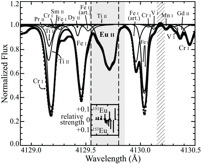
Figure 2.— The 4129-Å Eu ii line in the solar spectrum. Individual lines are annotated and are listed in Table 3. The hyperfine components (see § 3.1) appear in the inset plot, which is aligned with the wavelength scale of the main plot. The relative strengths of the 32 hyperfine components (Ivans et al., 2006) are plotted on a linear scale in the inset; the top half of the inset contains the components from the ¹⁵¹Eu isotope while the ¹⁵³Eu isotope components appear on the bottom. The gray box indicates the portion of the spectrum used to calculate $\chi^{2}$ during the abundance fitting step (see § 3.2). The cross-hatched region indicates a portion of the spectrum used to fit a continuum. This plot represents a subset of the spectral region used in our analysis; the full region is 5 Å wide and contains three additional continuum fitting regions.

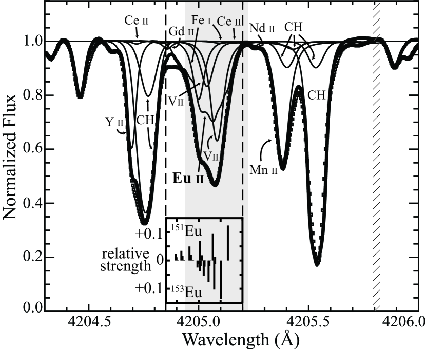
Figure 3.— The 4205-Å Eu ii line in the solar spectrum. Individual lines are annotated and are listed in Table 4. The hyperfine components (see § 3.1) appear in the inset plot, which is aligned with the wavelength scale of the main plot. The relative strengths of the 30 hyperfine components (Ivans et al., 2006) are plotted on a linear scale in the inset; the top half of the inset contains the components from the ¹⁵¹Eu isotope while the ¹⁵³Eu isotope components appear on the bottom. The gray box indicates the portion of the spectrum used to calculate $\chi^{2}$ during the abundance fitting step (see § 3.2). The cross-hatched region indicates a portion of the spectrum used to fit a continuum. This plot represents a subset of the spectral region used in our analysis; the full region is 8 Å wide and contains six additional continuum fitting regions.

Table 3Line list for the region near Eu ii at 4129 Å.

$\lambda$	Element	Lower Level	$\log{\textrm{\em gf}}$		$\Gamma_{6}$
(Å)		(eV)	solar fit	VALD	solar fit	VALD
4129.147	Pr ii	1.039	$-0.100$	$-0.100$	$-7.454$	…
4129.159	Cr i	3.013	$-1.948$	$-1.948$	$-6.964$	$-7.362$
4129.159	Ti ii	1.893	$-2.300$	$-1.730$	$-6.900$	$-7.908$
4129.166	Ti i	2.318	$-0.200$	$-0.231$	$-6.900$	$-7.572$
4129.174	Ce ii	0.740	$-3.000$	$-0.901$	$-7.493$	…
4129.182	Cr i	2.914	$-0.100$	…	$-8.300$	…
4129.220	Fe i	3.417	$-3.500$	$-2.030$	$-6.857$	$-7.255$
4129.220	Sm ii	0.248	$-1.123$	$-1.123$	$-7.536$	…
4129.425	Dy ii	0.538	$-0.522$	$-0.522$	$-7.554$	…
4129.426	Nb i	0.086	$-0.780$	$-0.780$	$-7.462$	…
4129.458	Fe i	3.396	$-1.950$	$-1.970$	$-6.863$	$-7.206$
4129.522	Fe i	3.140	$-3.497$	…	$-6.873$	…
4129.643	Ti i	2.239	$-1.987$	$-1.987$	$-7.529$	$-7.529$
4129.705	Eu ii	0.000	$+0.260$	$+0.173$	$-7.174$	…
4129.817	Co i	3.812	$-1.808$	$-1.808$	$-6.099$	$-7.782$
4129.837	Nd ii	2.024	$-0.543$	$-0.543$	$-6.237$	…
4129.959	Fe i	2.670	$-3.139$	…	$-7.322$	…
4130.035	Fe i	1.557	$-3.900$	$-4.345$	$-7.885$	$-7.826$
4130.036	Fe i	3.111	$-2.350$	$-2.636$	$-8.026$	$-7.857$
4130.073	Cr i	2.914	$-1.971$	$-1.971$	$-6.929$	$-7.349$
4130.122	V i	1.218	$-1.000$	$-3.142$	$-7.060$	$-7.800$
4130.233	Mn i	2.920	$-2.400$	$-3.309$	$-7.900$	$-7.784$
4130.315	V i	2.269	$-0.300$	$-0.607$	$-7.187$	$-7.585$
4130.364	Gd ii	0.731	$+0.177$	$-0.090$	$-6.608$	…
4130.452	Cr i	2.914	$-1.099$	$-2.751$	$-6.805$	$-7.348$

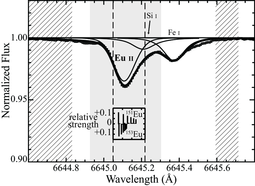
Figure 4.— The 6645-Å Eu ii line in the solar spectrum. Note that the ordinate axis is scaled differently than in Figures 2 and 3. Individual lines are annotated and are listed in Table 5. The hyperfine components (see § 3.1) appear in the inset plot, which is aligned with the wavelength scale of the main plot. The relative strengths of the 30 hyperfine components (Ivans et al., 2006) are plotted on a linear scale in the inset; the top half of the inset contains the components from the ¹⁵¹Eu isotope while the ¹⁵³Eu isotope components appear on the bottom. The gray box indicates the portion of the spectrum used to calculate $\chi^{2}$ during the abundance fitting step (see § 3.2). The two cross-hatched regions indicate the portion of the spectrum used to fit a continuum. This plot represents a subset of the spectral region used in our analysis; the full region is 5 Å wide and contains four additional continuum fitting regions.

Hyperfine splitting is the dominant broadening mechanism for the europium spectral lines. The interaction between the nuclear spin and the atom’s angular momentum vector causes energy level splitting in atoms with odd atomic numbers (europium is $Z=63$). The effect is particularly pronounced in rare earth elements. The 4129-Å and 4205-Å lines, for example, have FWHMs of 1.5 Å, due largely to hyperfine structure (but not isotope splitting—see insets of Figures 2–4). Since the relative strengths of the hyperfine components are constant without regard to temperature, pressure, or magnetic field (Abt, 1952), the components measured in laboratory settings can be applied to stellar spectra.

Like other spectral fitting packages, SME has no built-in treatment of hyperfine structure. We therefore convert a single europium line into its constituent hyperfine components and include them as separate entries in the star’s line list. The relative strengths and wavelength offsets of the hyperfine components come from Ivans et al. 2006, which bases the values on an FTS laboratory analysis. Following the procedure of Ivans et al. 2006, we assume a solar system composition for the relative abundance of the two europium isotopes (¹⁵¹Eu at 47.8% and ¹⁵³Eu at 52.2%, from Rosman & Taylor 1998). We divide the Eu ii $\log{\textrm{\em gf}}$ values listed in Tables 3, 4, and 5 amongst the hyperfine components according to their relative strengths. All other attributes of the Eu ii lines remain the same in the creation of the hyperfine lines. The relative strengths of the hyperfine components are displayed in the inset plots in the solar spectrum Figures 2, 3, and 4.

Table 4Line list for the region near Eu ii at 4205 Å.

$\lambda$	Element	Lower Level	$\log{\textrm{\em gf}}$		$\Gamma_{6}$
(Å)		(eV)	solar fit	VALD	solar fit	VALD
4204.695	Y ii	0.000	$-1.800$	$-1.760$	$-7.700$	…
4204.717	Ce ii	0.792	$-0.963$	$-0.963$	$-7.000$	…
4204.759	CH	0.519	$-1.140$	$-1.158$	$-8.900$	…
4204.771	CH	0.520	$-1.900$	$-1.135$	$-8.500$	…
4204.801	Sm ii	0.378	$-1.771$	$-1.771$	$-6.738$	…
4204.831	CH	0.520	$-3.360$	$-3.360$	$-7.699$	…
4204.858	Gd ii	0.522	$-0.668$	$-0.668$	$-6.787$	…
4204.990	Cr i	4.616	$-1.457$	$-1.457$	$-6.658$	$-7.852$
4205.000	Fe i	4.220	$-1.900$	$-2.150$	$-7.000$	$-7.548$
4205.038	V ii	1.686	$-1.850$	$-1.875$	$-6.800$	$-7.913$
4205.042	Eu ii	0.000	$+0.250$	$+0.120$	$-6.800$	…
4205.084	V ii	2.036	$-1.100$	$-1.300$	$-6.900$	$-7.956$
4205.098	Fe i	2.559	$-4.900$	$-4.900$	$-6.671$	$-7.865$
4205.107	Cr i	4.532	$-1.160$	$-1.160$	$-6.582$	$-7.776$
4205.163	Ce ii	1.212	$-0.653$	$-0.653$	$-6.672$	…
4205.253	Nd ii	0.680	$-0.992$	$-0.992$	$-6.699$	…
4205.303	Nb i	0.049	$-0.850$	$-0.850$	$-6.677$	…
4205.381	Mn ii	1.809	$-3.300$	$-3.376$	$-6.800$	$-8.001$
4205.402	CH	0.488	$-2.300$	$-3.960$	$-8.000$	…
4205.427	CH	1.019	$-2.300$	$-1.130$	$-8.000$	…
4205.491	CH	1.019	$-3.463$	$-3.463$	$-8.000$	…
4205.533	CH	1.019	$-1.800$	$-1.149$	$-8.000$	…
4205.538	Fe i	3.417	$-1.100$	$-1.435$	$-7.800$	$-7.224$

Table 5Line list for the region near Eu ii at 6645 Å.

$\lambda$	Element	Lower Level	$\log{\textrm{\em gf}}$		$\Gamma_{6}$
(Å)		(eV)	solar fit	VALD	solar fit	VALD
6644.320	CN	0.805	$-1.456$	$-2.258$	$-7.695$	…
6644.415	La i	0.131	$-1.330$	$-2.070$	$-8.000$	…
6645.111	Eu ii	1.380	$+0.219$	$+0.205$	$-7.218$	…
6645.210	Si i	6.083	$-2.510$	$-2.120$	$-7.118$	…
6645.372	Fe i	4.386	$-2.759$	$-3.536$	$-6.780$	$-7.808$

3.2. Europium Abundances

In order to measure the europium abundances in our selected stars, we begin with the co-added spectra described in § 2.2. We do a preliminary continuum fit using the SME routines, which follow the VF05 procedure: deep features are filled in with a median value from neighboring spectral orders, then a sixth-order polynomial is fit to the region of interest. The built-in procedure creates a flat, normalized continuum, though we find it necessary to fine-tune the continuum normalization in the course of our europium fitting.

From the VF05 SPOCS catalog we take $T_{\rm eff}$, $\log{g}$, [M/H], $v\sin{i}$, $v_{mac}$, and $v_{mic}$ (fixed at 0.85 km s^-1) for each star we consider. In general, the global parameters from VF05 agree very well with the values adopted in the studies we compare to here. (Most of the literature values fall within the 2-$\sigma$ errors quoted in VF05.) The VF05 catalog is one of the largest and most reliable sources of stellar properties determined to date; Haywood 2006, for example, finds the VF05 $T_{\rm eff}$ and [M/H] to be in good agreement with other reliable measurements.

For most element abundances we use a scaled solar system composition, shifting the Grevesse & Sauval 1998 solar abundances by the star’s [M/H]. The exceptions to this rule are sodium, silicon, titanium, iron, and nickel, which VF05 measured individually. Those $\alpha$ and iron-peak elements are therefore treated independently of the naïve scaled-solar adjustment. It is possible that a more explicit treatment of iron-peak and $\alpha$ elements would improve our europium measurement accuracy. For the present study, however, we deem individual abundance analysis (apart from europium) unnecessary. We hold fixed the abundances of all elements other than europium in the subsequent analysis.

We fit for the europium abundance by iterating three $\chi^{2}$-minimization routines that solve for the wavelength alignment, spectrum continuum, and europium abundance. A summary of each routine follows:

1. Wavelength. The pixel scale is pre-determined from the thorium lamp calibration taken each night. A first estimate of the rest frame wavelengths comes from a cross-correlation of the full spectral segment with the solar spectrum, a built-in functionality of SME. We then use a 2-Å region immediately surrounding the Eu ii line of interest to perform a $\chi^{2}$ minimization between the modeled stellar atmosphere and the spectral data, thus solving for the wavelength scale alignment as precisely as possible in the Eu ii region.

2. Continuum. We fit a quadratic function across the points designated in the solar spectrum as continuum-fitting points (the cross-hatch regions in Figures 2, 3, and 4). We adjust the quadratic continuum function vertically to require that 1–2% of spectral points in the full spectral segment are above unity, thereby ensuring that all spectra are scaled identically.

3. Abundance. We perform a $\chi^{2}$ minimization adjusting only the abundance of europium. We begin with the solar abundance value scaled by the star’s metallicity, then search $1.0\textrm{ dex}$ of europium abundance space to find the best-fit value. In minimizing the $\chi^{2}$ statistic, we calculate the residuals between the data and the fit in a limited region around the Eu ii line (the gray regions in Figures 2, 3, and 4).

The wavelength alignment, spectrum continuum, and europium abundance fitting routines are run in that order and iterated until a stable solution is reached. In most cases a stable solution requires only one or two iterations. The abundances for each line in each star as determined by this process are listed in Table 2.

After running our automatic europium fitting algorithm on all 41 stars, we examine each line in each star by eye to confirm that the fit is successful. In a few of the metal-poor 4129-Å fits, the blended lines that encroach on Eu ii were poorly enough fit with the VF05 SPOCS values that the europium value was unconvincing. In those cases, the 4129-Å value is omitted from Table 2 and does not contribute to the average. See Figure 5 for a comparison of a rejected 4129-Å feature and a robust 4129-Å fit. Similarly, in a few metal-poor stars the 6645-Å line is too weak to be seen in the noise, and hence the output of the fitting routine serves only as an upper limit on the europium abundance. See Figure 5 for a comparison of a measureable 6645-Å feature and a feature that provides an upper limit. In the cases where the 6645-Å line is an upper limit only, it is listed as such in Table 2 and does not contribute to the average.

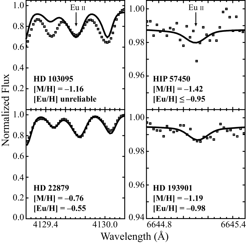
Figure 5.— Bad fits (top) versus good fits (bottom) in comparable stars. In the upper left panel, the SPOCS stellar properties fit the lines adjacent to Eu ii poorly enough that [Eu/H] is unreliable. That line is removed from further analysis. In the upper right panel, the 6645-Å line is buried in the noise, meaning the fit represents an upper limit to the europium abundance. The abundance upper limit is noted in Table 2, but does not contribute to the overall [Eu/H] measurement in the star. The lower two panels include fits to stars with similar characteristics to the stars in the upper panels, but where the 4129-Å and 6645-Å fits were more successful.

If both 4129 Å and 6645 Å proved problematic we removed the star from our analysis entirely. The three stars for which this was the case (listed in § 2.1) are omitted from Tables 1 and 2. Since all of the rejected stars were metal poor, we conclude that our fitting routine is most robust at solar metallicity, and becomes less reliable at [M/H] $<-1$. Temperature may also play a role, as one of the rejected stars, HD 64090, has $T_{\rm eff}=7300\textrm{ K}$; VF05 determined SME to be reliable between 4800 and $6500\textrm{ K}$.

For each star we calculate a weighted average europium abundance value based on the three (or, in some cases, two) spectral lines. Weighting the average is important because for stars with relatively few observations (e.g., HD 156365 in Figure 1), the weak line at 6645 Å should be weighted significantly less than the more robust blue lines. Stars with a larger number of observations and higher S/N spectra (e.g., HD 144585 in Figure 1) should have the 6645-Å line weighted more strongly. In order to determine the relative weights of the three spectral lines, we tested the robustness of our fit by adding artificial noise to the spectra. We describe that process in § 3.3.

3.3. Error Analysis

We begin our error analysis by adding to the data Gaussian-distributed random noise with a standard deviation set by the photon noise at each pixel. We then fit the europium line again, using the same iterative $\chi^{2}$-minimization process described in § 3.2, and repeat the process 50 times. The standard deviation of the 50 Monte Carlo trials determines the relative weights of the lines in the average listed in Table 2, with lower standard deviation lines (corresponding to a more robust fit) weighted more strongly.

As expected, the results of the Monte Carlo trials show that the larger the photon noise in an observation, the less that line is to be weighted. We derive a linear relation between the Poisson uncertainty of an observation and its relative weight, based on the Monte Carlo results. Because the Monte Carlo trials are CPU intensive, we plan to use that relation to determine relative weights in the future.

We estimate the uncertainty of our europium abundances to be the sum of the squares of the residuals for all three lines, where we assign the residuals the same relative weights we applied when calculating the average. We also impose an error floor of $0.02\textrm{ dex}$, added to the uncertainty in quadrature.

The error floor comes from a comparison of abundance values from the individual lines (Figure 6, discussed in more detail in § 4.1); error bars of $0.03\textrm{ dex}$ on each measurement would make the reduced $\sqrt{\chi^{2}}$ $=1$. A minimum error of $0.03\textrm{ dex}$ on each europium measurement translates into an uncertainty of $0.02\textrm{ dex}$ for the final averaged value. The $0.02\textrm{ dex}$ error floor is included in the uncertainty quoted in Table 2.

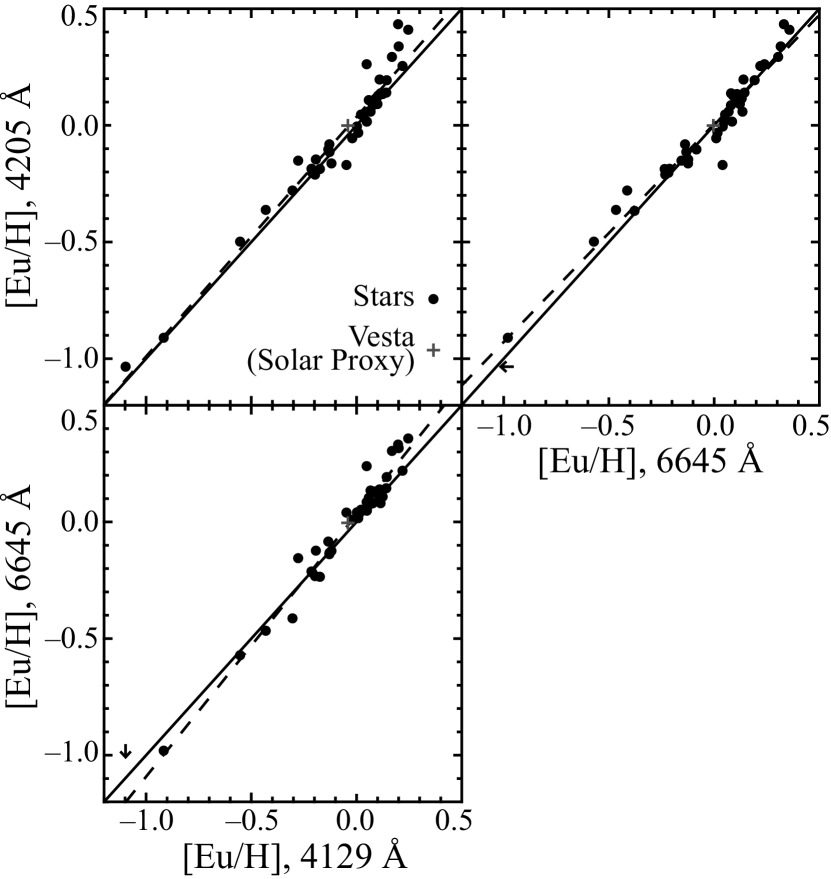
Figure 6.— A comparison of the Eu ii values measured in the 41 stars of this study, as listed in Table 2. Vesta is marked with a plus symbol. The solid line represents a 1:1 correlation; the dashed line is a best fit to the data. Points are omitted where the fit was poor in one of the Eu ii lines. Upper limits for the 6645-Å line are marked with arrows. See § 4.1 for a discussion of the quality of the fit.

As an initial test of the robustness of our fitting routine, we measure the europium abundance in a spectrum of Vesta, which serves as a solar proxy. The values are listed in the last row of Table 2. The three Vesta europium abundances have a standard deviation of $0.022\textrm{ dex}$, indicating that systematic errors ($\sim$ $0.03\textrm{ dex}$ for Vesta, its offset from the solar value) may be a significant portion of the error budget.

For the moment we absorb any systematic error with our random error estimates. The full sample of 1000 stars, the analysis of which will follow this work, will allow a far more thorough investigation of the dependence of our results on various model parameters ($T_{\rm eff}$, $\log{g}$, etc.) than can be accomplished here. Therefore, we delay a substantive discussion of systematics until we have more europium abundance measurements in hand, though we touch on it again in § 4.1 and § 4.2. It is important to note that since most of the CCPS stars are similar to the Sun, and we are treating each star identically, our results will be internally consistent.

3.4. Notes on Individual Lines

3.4.1 Europium 4129 Å

The europium line at 4129 Å is the result of a resonance transition of Eu ii, and is a strong, relatively clean line. It provides the most reliable measurement of europium abundance in a star. Our fit to the Eu ii line at 4129 Å in the solar spectrum (described in § 3.1) appears as Figure 2, with the 32 hyperfine components (16 each from ¹⁵¹Eu and ¹⁵³Eu; Ivans et al. 2006) represented in the Figure 2 inset.

In the course of stellar fitting, the europium abundance is determined from the 4129 Å line in all 41 stars except HD 103095. That star is quite metal poor ([M/H] $=-1.16$) and cool ($T_{\rm eff}=4950$), factors that likely contribute to the poor fit in the lines adjacent to the Eu ii line of interest (see Figure 5).

3.4.2 Europium 4205 Å

The Eu ii line at 4205 Å is the other fine-structure component of the resonance transition responsible for the line at 4129 Å. Though it is as strong as the Eu ii line at 4129 Å, contamination from embedded lines (see Figure 3) has the potential make the 4205-Å line less reliable. However, it is useful as a comparison line for the results from the 4129-Å Eu ii line. Our solar spectrum fit at 4205 Å appears in Figure 3, with the 30 hyperfine components (15 each from ¹⁵¹Eu and ¹⁵³Eu; Ivans et al. 2006) in the inset. Despite its blended nature, the fit appears sound in all 41 stars.

3.4.3 Europium 6645 Å

The Eu ii line at 6645 Å is weaker than the lines in the blue, but it is also relatively unblended, making it worthwhile to fit wherever possible. Our solar spectrum fit at 6645 Å appears in Figure 4, with the inset plot showing the 30 hyperfine components (15 each from ¹⁵¹Eu and ¹⁵³Eu; Ivans et al. 2006). In HIP 57450, which is metal poor ([M/H] $=-1.42$) and has only one observation, the 6645-Å line was lost in the noise (see Figure 5), and only the 4129-Å and 4205-Å lines contribute to the final europium abundance; the 6645-Å line provides an upper limit only.

4. Results

4.1. Comparison of Individual Lines

We compare our results from the three Eu ii lines in Figure 6. The Vesta abundances, included as a solar proxy, are consistent with the stellar abundances to within $0.03\textrm{ dex}$. By assigning a measurement uncertainty of $0.03\textrm{ dex}$ to each line, the reduced $\sqrt{\chi^{2}}$ for each of the three plots is unity. This measurement uncertainty is the source of the error floor discussed in § 3.3.

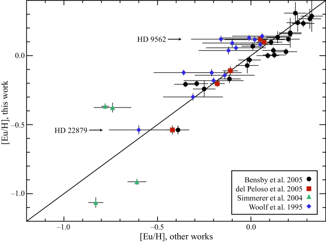
Figure 7.— A comparison of the final Eu ii values from this work with literature measurements. The solid line represents a 1:1 correlation. The horizontal error bars represent the uncertainties as quoted in the source literature. The vertical error bars come from our analysis as described in § 3.3. Two stars, HD 9562 and HD 22879 (with [Eu/H] of $+0.12$ and $-0.54$, respectively), were included in the Bensby et al. 2005, del Peloso et al. 2005, and Woolf et al. 1995 analyses, so those two stars are represented by three points along the abscissa at the same ordinate value. See Table 1 for the full list of the europium abundances plotted here, and see § 4.2 for a discussion of the quality of our fit based on this plot.

Calculating the best-fit line for each comparison plot (the dashed lines in Figure 6) lends insight into possible systematic trends in our analysis. In the blue, the two Eu ii lines (4129 Å and 4205 Å) have no apparent linear systematic trend: the slope of the best-fit line is 1.03. The red Eu ii line (6645 Å), however, exhibits a minor systematic trend: the best-fit line in the red has a slope of 1.10 relative to the blue, i.e., a 10% stretching of the blue abundance values about [Eu/H] $=0$ roughly reproduces the red abundance values. Since this systematic trend is absorbed by the $0.03\textrm{ dex}$ error bars assigned to each point (necessary to make reduced $\sqrt{\chi^{2}}$ unity even when comparing the non-systematic blue lines), we make no attempt to correct this systematic trend here.

Between the relatively low measurement uncertainty needed to achieve reduced $\sqrt{\chi^{2}}$ of unity and the minor systematic trend that only appears in the red, we conclude that the europium abundance values derived from the Eu ii lines at 4129 Å, 4205 Å, and 6645 Å are consistent with one another.

4.2. Comparison with Literature Europium Measurements

In Figure 7, we compare our final europium abundance measurements to the literature values. The agreement is quite good. The literature values, plotted with the error bars quoted in the original studies, appear as the abscissa. Our europium values, plotted with the error bars calculated in § 3.3 and listed in Table 2, appear as the ordinate. The solid line represents a 1:1 correlation. Comparing the points to the 1:1 line, the reduced $\sqrt{\chi^{2}}$ $=2.78$. That value is dominated by HD 103095, the Simmerer et al. 2004 data point with the smallest error bars, and omitting it makes the reduced $\sqrt{\chi^{2}}$ $=1.57$.

Adopting the global values ($T_{\rm eff}$, [M/H], $\log{g}$) used by the comparison studies (instead of the VF05 values) drops the reduced $\sqrt{\chi^{2}}$ to 1.93, indicating that some of the scatter in Figure 7 is from the choice of stellar parameters. We emphasize that the VF05 stellar parameters are reliable; we calculate reduced $\sqrt{\chi^{2}}$ using the comparison studies’ values in an attempt to separate how much of the disagreement in Figure 7 is from the europium abundance technique and how much is from the parameters adopted.

Omitting the outlier mentioned at the beginning of this section, we examine the data in Figure 7 to search for systematics in our results relative to the literature values. We consider the effects of a global offset in our europium values and a linear trend with europium abundance, finding that systematic offsets of $\sim$ $0.1\textrm{ dex}$ and linear trends of $\sim$ $40\%$ are needed to make reduced $\sqrt{\chi^{2}}$ climb to 2. We conclude that our error bars have sufficiently characterized our uncertainties.

Overall, we find reduced $\sqrt{\chi^{2}}$ to be dominated by the points at [Eu/H] $<0.5$, consistent with our conclusion in § 3.2 that our results are most reliable near solar metallicities, although the larger error bars on the Woolf et al. 1995 points make the correlation very forgiving near [Eu/H] $=0$. Our spectra have very high S/N: $\sim$ 160 at 4200 Å in a single observation, enhanced substantially by our co-adding procedure (§ 2.2). The automated SME synthesis treats all stars consistently, especially important for line blends in the crowded blue regions. For these reasons we believe that our europium abundance technique is accurate and robust and that our smaller error bars are warranted.

We conclude that our abundance measurements are consistent with previous studies, not surprising since most abundance techniques rely on the same Kurucz stellar atmosphere models. Because the majority of the points in Figures 7 fall near the 1:1 correlation, we also conclude that near [Eu/H] $=0$ our errors are $\sim$ $0.03\textrm{ dex}$, though at [Eu/H] $<-0.5$, the errors may be as high as $0.1\textrm{ dex}$.

5. Summary

We have established that our method for measuring europium in solar-metallicity stars using SME is sound. The resolution and S/N of the Keck HIRES spectra are sufficiently high to fit the Eu ii lines in question. The values obtained from the three europium lines are self-consistent, and our final averaged europium value for each of the 41 stars in this study are consistent with the literature values for those stars.

By employing SME to calculate our synthetic spectra, we are self-consistently modeling all the lines in the regions of interest. Any blending from neighboring lines is treated consistently from star to star, adding robustness to our europium determination. Using SME has the added benefit of allowing us to adopt the stellar parameters from the SPOCS catalog. Our automated procedure ensures all stars are treated consistently.

Having established a new method for measuring stellar europium abundances, we intend to apply our technique to 1000 F, G, and K stars from the Keck CCPS survey. Our analysis of europium in these stars will represent the largest and most consistent set of europium measurements in solar-metallicity stars to date, and will provide insight into the question of the r-process formation site and the enrichment history of the Galaxy.

References

- Abt (1952) Abt, A. 1952, ApJ, 115, 199
- Barklem et al. (2000) Barklem, P. S., Piskunov, N., & O’Mara, B. J. 2000, A&AS, 142, 467
- Bensby et al. (2005) Bensby, T., Feltzing, S., Lundström, I., & Ilyin, I. 2005, A&A, 433, 185
- Burris et al. (2000) Burris, D. L., Pilachowski, C. A., Armandroff, T. E., Sneden, C., Cowan, J. J., & Roe, H. 2000, ApJ, 544, 302
- del Peloso et al. (2005) del Peloso, E. F., da Silva, L., & Porto de Mello, G. F. 2005, A&A, 434, 275
- ESA (1997) ESA. 1997, The Hipparcos and Tycho catalogues, Garching
- Frebel et al. (2007) Frebel, A., Christlieb, N., Norris, J. E., Thom, C., Beers, T. C., & Rhee, J. 2007, ApJ, 660, L117
- Grevesse & Sauval (1998) Grevesse, N., & Sauval, A. J. 1998, Space Science Reviews, 85, 161
- Haywood (2006) Haywood, M. 2006, MNRAS, 371, 1760
- Ivans et al. (2006) Ivans, I. I., Simmerer, J., Sneden, C., Lawler, J. E., Cowan, J. J., Gallino, R., & Bisterzo, S. 2006, ApJ, 645, 613
- Johnson & Bolte (2001) Johnson, J. A., & Bolte, M. 2001, ApJ, 554, 888
- Kibrick et al. (2006) Kibrick, R. I., Clarke, D. A., Deich, W. T. S., & Tucker, D. 2006, in Society of Photo-Optical Instrumentation Engineers (SPIE) Conference Series, Vol. 6274, Society of Photo-Optical Instrumentation Engineers (SPIE) Conference Series
- Koch & Edvardsson (2002) Koch, A., & Edvardsson, B. 2002, A&A, 381, 500
- Kupka et al. (1999) Kupka, F., Piskunov, N., Ryabchikova, T. A., Stempels, H. C., & Weiss, W. W. 1999, A&AS, 138, 119
- Kurucz (1992) Kurucz, R. L. 1992, in IAU Symposium, Vol. 149, The Stellar Populations of Galaxies, ed. B. Barbuy & A. Renzini, 225
- Kurucz et al. (1984) Kurucz, R. L., Furenlid, I., Brault, J., & Testerman, L. 1984, Solar flux atlas from 296 to 1300 nm (National Solar Observatory Atlas, Sunspot, New Mexico: National Solar Observatory, 1984)
- Lai et al. (2008) Lai, D. K., Bolte, M., Johnson, J. A., Lucatello, S., Heger, A., & Woosley, S. E. 2008, ApJ, 681, 1524
- Marcy & Butler (1992) Marcy, G. W., & Butler, R. P. 1992, PASP, 104, 270
- Marcy et al. (2008) Marcy, G. W., Butler, R. P., Vogt, S. S., Fischer, D. A., Wright, J. T., Johnson, J. A., Tinney, C. G., Jones, H. R. A., Carter, B. D., Bailey, J., O’Toole, S. J., & Upadhyay, S. 2008, Physica Scripta Volume T, 130, 014001
- Moore et al. (1966) Moore, C. E., Minnaert, M. G. J., & Houtgast, J. 1966, The solar spectrum 2935 A to 8770 A (National Bureau of Standards Monograph, Washington: US Government Printing Office (USGPO), 1966)
- Piskunov et al. (1995) Piskunov, N. E., Kupka, F., Ryabchikova, T. A., Weiss, W. W., & Jeffery, C. S. 1995, A&AS, 112, 525
- Reddy et al. (2006) Reddy, B. E., Lambert, D. L., & Allende Prieto, C. 2006, MNRAS, 367, 1329
- Rosman & Taylor (1998) Rosman, K. J. R., & Taylor, P. D. P. 1998, Journal of Physical and Chemical Reference Data, 27, 1275
- Simmerer et al. (2004) Simmerer, J., Sneden, C., Cowan, J. J., Collier, J., Woolf, V. M., & Lawler, J. E. 2004, ApJ, 617, 1091
- Sneden et al. (2008) Sneden, C., Cowan, J. J., & Gallino, R. 2008, ARA&A, 46, 241
- Valenti & Fischer (2005) Valenti, J. A., & Fischer, D. A. 2005, ApJS, 159, 141
- Valenti & Piskunov (1996) Valenti, J. A., & Piskunov, N. 1996, A&AS, 118, 595
- Vogt et al. (1994) Vogt, S. S., Allen, S. L., Bigelow, B. C., Bresee, L., Brown, B., Cantrall, T., Conrad, A., Couture, M., Delaney, C., Epps, H. W., Hilyard, D., Hilyard, D. F., Horn, E., Jern, N., Kanto, D., Keane, M. J., Kibrick, R. I., Lewis, J. W., Osborne, J., Pardeilhan, G. H., Pfister, T., Ricketts, T., Robinson, L. B., Stover, R. J., Tucker, D., Ward, J., & Wei, M. Z. 1994, in Presented at the Society of Photo-Optical Instrumentation Engineers (SPIE) Conference, Vol. 2198, Proc. SPIE Instrumentation in Astronomy VIII, David L. Crawford; Eric R. Craine; Eds., Volume 2198, p. 362, ed. D. L. Crawford & E. R. Craine, 362
- Wallace et al. (1998) Wallace, L., Hinkle, K., & Livingston, W. 1998, An atlas of the spectrum of the solar photosphere from 13,500 to 28,000 cm-1 (3570 to 7405 Å) (Tucson, AZ: National Optical Astronomy Observatories)
- Woolf et al. (1995) Woolf, V. M., Tomkin, J., & Lambert, D. L. 1995, ApJ, 453, 660