Unsterile-Active Neutrino Mixing: Consequences on Radiative Decay and Bounds from the X-ray Background

Abstract

We consider a sterile neutrino to be an unparticle, namely an unsterile neutrino, with anomalous dimension $\eta$ and study its mixing with a canonical active neutrino via a see-saw mass matrix. We show that there is no unitary transformation that diagonalizes the mixed propagator and a field redefinition is required. The propagating or “mass” states correspond to an unsterile-like and active-like mode. The unsterile mode features a complex pole or resonance for $0\leq\eta<1/3$ with an “invisible width” which is the result of the decay of the unsterile mode into the active mode and the massless particles of the hidden conformal sector. For $\eta\geq 1/3$, the complex pole disappears, merging with the unparticle threshold. The active mode is described by a stable pole, but “inherits” a non-vanishing spectral density above the unparticle threshold as a consequence of the mixing. We find that the radiative decay width of the unsterile neutrino into the active neutrino (and a photon) via charged current loops, is suppressed by a factor $\sim\Big{[}2\sin^{2}(\theta_{0})\,\frac{M^{2}}{\Lambda^{2}}\Big{]}^{\frac{\eta}{1-\eta}}$, where $\theta_{0}$ is the mixing angle for $\eta=0$, $M$ is approximately the mass of the unsterile neutrino and $\Lambda\gg M$ is the unparticle-scale. The suppression of the radiative (visible) decay width of the sterile neutrino weakens the bound on the mass and mixing angle from the X-ray or soft gamma-ray background.

I Introduction

Neutrino masses and oscillations are now an established phenomenon and an undisputable evidence of physics beyond the standard model. Although the origin and scale of masses remains a challenging question, the see-saw mechanism provides a compelling explanation of small active neutrino masses as the result of ratios of widely different scales seesaw . Among extensions of the standard model, the addition of sterile neutrinos, namely SU(2) singlets with a mass in the few keV range, acquires particular importance as a potential warm dark matter candidate dw ; colombi ; este ; shapo ; kusenko ; kusepetra ; petra ; coldmatter ; micha ; boysnudm ; kuseobs ; hector ; wu and could provide possible solutions to a host of astrophysical problems kusenko . The radiative decay pal of a sterile-like neutrino mass eigenstate into an active-like mass eigenstate and a photon leads to a decay line that could be observable in the X-ray or soft gamma ray background dolgov . The non-observation of this line provides a constraint on the mass and mixing angle of sterile-like neutrinos dolgov ; sorensen ; aba ; kuseobs ; micha ; hansen .

More recently sterile neutrinos with mass in the $\mathrm{GeV}$ range have been proposed as explanations of two seemingly unrelated and unexpected phenomena: an excess of air shower events at the SHALON gamma ray telescope, in a configuration where the expected number of events is negligible shalon , and as a potential explanation of the MiniBoone anomaly miniboone , namely the prominent peak of electron-neutrino events above background for $300\,\mathrm{MeV}\leq E_{\nu}\leq 475\,\mathrm{MeV}$. Sterile neutrinos in a three-active, two-sterile ($3+2$) oscillation scheme were proposed in Ref. maltoni as a possible explanation of the MiniBooNE anomaly, and an alternative explanation invoking the radiative decay of a heavy sterile neutrino with a small magnetic moment was proposed in Ref. gninenko .

In this article we study the possibility that sterile neutrinos are a manifestation of unparticles, which then mix with the active neutrinos via a see-saw-type mass matrix.

In a recent series of articles, Georgi georgi suggested an extension of the standard model in which particles couple to a conformal sector with a non-trivial infrared fixed point acquiring (large or non-perturbative) anomalous dimensions with potentially relevant consequences, some of which may be tested at the Large Hadron Collider (LHC) cheung ; raja ; quiros . Early work by Banks and Zaks banks provides a realization of a conformal sector emerging from a renormalization flow toward the infrared below an energy scale $\Lambda$ through dimensional transmutation, and supersymmetric QCD may play a similar role fox . Below this scale there emerges an effective interpolating field, the unparticle field, that features an anomalous scaling dimension georgi .

Various studies recognized important phenomenological georgi ; cheung ; spin12 ; ira ; Liao:2007ic astrophysical raffelt ; deshpande ; freitas and cosmological macdonald ; davo ; lewis ; kame ; he ; kiku ; xuelei ; rich consequences of unparticles, including Hawking radiation into unparticles dai , aspects of CP-violation zwicky1 , flavor physics flavor and low energy parity violation parity . More recently, the consequences of mixing of unparticle scalar fields and a Higgs field were studied in Ref. unparticleus with implications for slow-roll inflation.

A deconstruction program describes the unparticle as a tower of a continuum of excitations step . However, this is not the only interpretation of unparticles. As mentioned in Ref. unparticleus , anomalous scaling dimensions are ubiquitous in critical phenomena near an infrared fixed point amit ; brezin , which is the main observation in Ref. banks . There is also a well known phenomenon in QCD Neubert:2007kh where anomalous dimensions emerge from the multiple emission and absorption of gluons as a result from the resummation of infrared Sudakov logarithms. Similarly, in QED, Bloch-Nordsieck resummation of infrared divergences arising from multiple emissions and absorptions of photons yield threshold infrared divergences and lead to a renormalized electron propagator that also features anomalous dimensions bloch ; bogo . The renormalization group resummation of absorption and emission of massless quanta lead quite generally to anomalous dimensions in the propagators infradiv .

A recent study liliu suggests a connection between unparticles and the Miniboone anomaly, namely, that the heaviest mass eigenstates corresponding to the mixed $\nu_{\mu}-\nu_{e}$ decays into the lightest eigenstate and a scalar unparticle (see also Zhou:2007zq ). Furthermore, unparticle contributions to the neutrino-nucleon cross section and its influence on the neutrino flux expected in a neutrino telescope such as IceCube have been reported in Ref. telescopes .

If heavy sterile neutrinos decaying into lighter active neutrinos and massless particles of a hidden conformal sector described by scalar unparticles are a plausible explanation of the MiniBooNE anomaly, then the coupling of the sterile neutrinos to this degree of freedom will necessarily lead to the consideration of the sterile neutrino itself being an unparticle.

This consideration emerges naturally from the “deconstruction” argument step , since the coupling of the sterile neutrino to the scalar unparticle leads to a spectral representation of the sterile neutrino propagator that features anomalous scaling dimensions. Alternatively, (but equivalently) the emission and absorption of massless (conformal) quanta lead to infrared threshold divergences akin to Sudakov logarithms whose renormalization group (or Bloch-Nordsieck bloch ) resummation leads to anomalous dimensions Neubert:2007kh ; infradiv .

Massive fermionic unparticles with a soft conformal breaking mass term had been introduced in Ref. terning and a very interesting proposal in which right handed neutrinos are fermionic unparticles was considered in Ref. conformalquiros .

If unparticle physics proves to be an experimentally relevant extension of the standard model, it is natural to consider sterile neutrinos, namely $SU(2)$ singlets, as being unparticles, and we refer to them as unsterile neutrinos.

Unsterile neutrinos are assumed to couple to a “hidden” conformal sector beyond the standard model and acquire a (possibly large) anomalous scaling dimension below a scale $\Lambda$ of dimensional transmutation at which the infrared fixed point of the conformal sector dominates the low energy dynamics.

In this article we consider such a possibility and study the consequences of unsterile neutrinos mixing with active neutrinos via a typical see-saw mass matrix. We consider the simplest scenario of one unsterile and one active Dirac neutrino to establish the general consequences of their mixing. Our objectives in this article are two-fold:

• Because unsterile neutrinos feature non-canonical kinetic terms, novel aspects of mixing phenomena emerge. We explore the fundamental aspects of mixing between these unsterile and the usual active neutrinos via a see-saw type mass matrix.

• We also focus on potential cosmological consequences, in particular if and how the unparticle nature of a sterile neutrino modifies its radiative decay into an active-like neutrino. This decay rate is an important ingredient to establish bounds on masses and mixing angles from the cosmological X-ray or soft-gamma background in the case when the mass of the sterile-like neutrino is in the keV range, which is of interest when considering it as a dark matter candidate.

Our results can be summarized as the following:

• The spinor nature of the unparticle field introduces novel aspects of mixing, in which there is no unitary transformation purely in flavor space that diagonalizes the full propagator. The diagonalization requires a non-unitary transformation and field redefinition followed by a momentum-dependent transformation that is unitary below the unparticle threshold but non-unitary above. The resulting mixing angles depend on the four-momentum.

• For a see-saw type mass matrix that mixes the unsterile and active neutrino, we find an unsterile-like mode with an “invisible” decay width. A renormalization group inspired “resummation” argument suggests that this width is a result of the decay of the unsterile-like mode into the active-like mode and particles in the “hidden sector”. A complex pole for the unsterile mode exists only for $0<\eta\leq 1/3$, where $\eta$ is the unparticle anomalous dimension. As $\eta\rightarrow 1/3^{-}$ the real part of the pole approaches the unparticle threshold from above and the width becomes large. For $\eta>1/3$ the spectral density for the unsterile mode does not feature a complex pole, but is described by a broad continuum with a large enhancement at the unparticle threshold.

  The active-like mode features a stable isolated pole below the unparticle threshold, but “inherits” a non-trivial spectral density above it as a consequence of the mixing, even in absence of standard model interactions. The non-vanishing spectral density may open up new kinematic channels for weak interactions.

• We obtain the radiative decay width of the unsterile-like mode into the active-like mode and a photon via a charged current loop. For large anomalous dimension (but $\eta<1/3$) we find a substantial suppression of the radiative decay width suggesting a concomitant weakening of the bounds on the mass and mixing angle from the X-ray or soft gamma ray background.

II unsterile-active mixing

In order to study the fundamental aspects of unsterile-active neutrino mixing and the potential cosmological consequences, we consider the simplest case with one unsterile and one active Dirac neutrino. The case of Majorana neutrinos and a triplet of unsterile neutrinos as envisaged in extensions beyond the standard model micha will be studied in detail elsewhere.

For an unsterile Dirac fermion the Lagrangian density in momentum space is fox ; terning

$$\mathcal{L}=\overline{\psi}_{U}(-p)\,\big{(}\not\!{p}-M\big{)}F(p)\,\psi_{U}(p),$$ (1)

where

$$F(p)=\Big{[}\frac{-p^{2}+M^{2}-i\epsilon}{\Lambda^{2}}\Big{]}^{-\eta}~{}~{};~{}~{}0\leq\eta<1\,.$$ (2)

$\Lambda$ is the scale below which the low energy dynamics is dominated by the infrared fixed point of the conformal sector. Below this scale the unparticle is described by an interpolating field whose two point correlation function scales with an anomalous dimension georgi . Consistency of the unparticle interpretation requires that

$$M<\Lambda\,.$$ (3)

We consider the mixing with an “active” massless Dirac neutrino $\psi_{a}$ of the form

$$\mathcal{L}_{m}=\overline{\psi}_{U}\,m\,\psi_{a}+\mathrm{h.c.}$$ (4)

A see-saw mechanism consistent with the unparticle nature of the sterile neutrino, namely an interpolating effective field below a scale $\Lambda$ entails the following hierarchy of scales

$$m\ll M<\Lambda\,.$$ (5)

In what follows we will explicitly invoke this hierarchy in the analysis.

It is convenient to introduce the “flavor doublet”

$$\Psi=\Big{(}\begin{array}[]{c}\psi_{a}\\ \psi_{U}\end{array}\Big{)},$$ (6)

and write the Lagrangian density for the unsterile and active fermions as

$$\mathcal{L}=\overline{\Psi}(-p)\,\Big{[}\not\!{p}\,\mathds{F}-\mathds{M}\Big{]}\,\Psi(p),$$ (7)

where

$$\mathds{F}=\Bigg{(}\begin{array}[]{cc}1&0\\ 0&F(p)\end{array}\Bigg{)},$$ (8)

and

$$\mathds{M}=\Bigg{(}\begin{array}[]{cc}0&m\\ m&MF(p)\end{array}\Bigg{)}.$$ (9)

The equation of motion is

$$\Big{[}\not\!{p}\,\mathds{F}-\mathds{M}\Big{]}\,\Psi(p)=0.$$ (10)

It is convenient to introduce the spinor $\Phi$ so that

$$\Psi(p)=\Big{[}\not\!{p}\,\mathds{I}+\mathds{F}^{-1}\,\mathds{M}\Big{]}\,\Phi(p),$$ (11)

which obeys the following equation of motion

$$\Big{[}p^{2}\mathds{F}-\mathds{M}~{}\mathds{F}^{-1}~{}\mathds{M}\Big{]}\Phi(p)=0,$$ (12)

where

$$\mathds{M}~{}\mathds{F}^{-1}~{}\mathds{M}=\Bigg{(}\begin{array}[]{cc}\frac{m^{2}}{F(p)}&~{}~{}mM\\ mM&~{}~{}m^{2}+M^{2}F(p)\end{array}\Bigg{)}.$$ (13)

The matrix in (12) can be written as follows

$$\Big{[}p^{2}\mathds{F}-\mathds{M}~{}\mathds{F}^{-1}~{}\mathds{M}\Big{]}=\alpha(p)~{}\mathds{I}-\beta(p)\Bigg{(}\begin{array}[]{cc}-\mathcal{C}(p)&\mathcal{S}(p)\\ \mathcal{S}(p)&\mathcal{C}(p)\end{array}\Bigg{)}\,.$$ (14)

Introducing the shorthand

$$Q=p^{2}-\frac{m^{2}}{F(p)}\,,$$ (15)

we obtain

$$\alpha(p) = \frac{1}{2}\Bigg{[}Q+F(p)(Q-M^{2})\Bigg{]}\,,$$ (16)

$$\beta(p) = \frac{1}{2}\Bigg{[}\Big{[}Q-F(p)(Q-M^{2})\Big{]}^{2}+4m^{2}M^{2}\Bigg{]}^{\frac{1}{2}}\,,$$ (17)

and

$$\mathcal{C}(p) = \frac{\Big{[}Q-F(p)(Q-M^{2})\Big{]}}{2~{}\beta(p)}\,,$$ (18)

$$\mathcal{S}(p) = \frac{mM}{\beta(p)}\,.$$ (19)

These functions obey

$$\mathcal{C}^{2}(p)+\mathcal{S}^{2}(p)=1\,.$$ (20)

It becomes clear that the dispersions relations for the propagating modes correspond to

$$\mathrm{det}\Big{[}p^{2}\mathds{F}-\mathds{M}~{}\mathds{F}^{-1}~{}\mathds{M}\Big{]}=\alpha^{2}(p)-\beta^{2}(p)=0\Rightarrow Q(Q-M^{2})-\frac{m^{2}M^{2}}{F(p)}=0,$$ (21)

which then leads to a self-consistent equation for the dispersion relation of the propagating modes

$$p^{2}_{\pm}=\frac{m^{2}}{F(p_{\pm})}+\frac{M^{2}}{2}\Bigg{[}1\pm\sqrt{1+\frac{4m^{2}}{M^{2}F(p_{\pm})}}~{}\Bigg{]}.$$ (22)

The Klein-Gordon operator (14), which we obtained from squaring the Dirac operator, can be diagonalized using the transformation

$$\mathcal{U}(p)=\Bigg{(}\begin{array}[]{cc}c(p)&s(p)\\ -s(p)&c(p)\end{array}\Bigg{)},$$ (23)

where

$$c(p)=\frac{1}{\sqrt{2}}\Big{[}1+\mathcal{C}(p)\Big{]}^{\frac{1}{2}}~{}~{};~{}~{}s(p)=\frac{1}{\sqrt{2}}\Big{[}1-\mathcal{C}(p)\Big{]}^{\frac{1}{2}}\,.$$ (24)

The resulting spinor is given by

$$\tilde{\Phi}(p)=\mathcal{U}^{-1}(p)\,\Phi(p)\,,$$ (25)

and in this basis, the Klein-Gordon matrix (14) becomes

$$\mathcal{U}^{-1}(p)\Big{[}p^{2}\mathds{F}-\mathds{M}~{}\mathds{F}^{-1}~{}\mathds{M}\Big{]}\mathcal{U}(p)=\Bigg{(}\begin{array}[]{cc}\alpha(p)+\beta(p)&0\\ 0&\alpha(p)-\beta(p)\end{array}\Bigg{)}.$$ (26)

An alternative manner to understand the solutions to the equations of motion is by going to the chiral representation. We do this by expressing the spinor $\Psi$ in terms of its right and left components, each a flavor doublet

$$\Psi=\Bigg{(}\begin{array}[]{c}\Psi_{R}\\ \Psi_{L}\end{array}\Bigg{)}.$$ (27)

We can then expand the right and left components in the helicity basis

$$\Psi_{R,L} = \sum_{h=\pm 1}v^{h}(\vec{p})\otimes\xi^{h}_{R,L}\,,$$ (28)

where

$$\frac{\vec{\sigma}\cdot\vec{p}}{|\vec{p}|}~{}v^{h}(\vec{p})=h~{}v^{h}(\vec{p})~{}~{};~{}~{}h=\pm 1,$$ (29)

and $\xi^{h}_{R,L}$ are flavor doublets. We find that

$$(p^{0}-h|\vec{p}|)\mathds{F}~{}\xi^{h}_{R}+\mathds{M}~{}\xi^{h}_{L} = 0,$$ (30)

$$(p^{0}+h|\vec{p}|)\mathds{F}~{}\xi^{h}_{L}+\mathds{M}~{}\xi^{h}_{R} = 0\,.$$ (31)

Using (31), we can expres $\xi^{h}_{L}$ in terms of $\xi^{h}_{R}$ and obtain

$$\Bigg{[}p^{2}\mathds{F}-\mathds{M}~{}\mathds{F}^{-1}~{}\mathds{M}\Bigg{]}\xi^{h}_{R}=0~{}~{};~{}~{}\xi^{h}_{L}=-\frac{\mathds{F}^{-1}~{}\mathds{M}}{(p^{0}+h|\vec{p}|)}~{}\xi^{h}_{R}\,.$$ (32)

Alternatively, we can express $\xi^{h}_{R}$ in terms of $\xi^{h}_{L}$ using (30), and obtain

$$\Bigg{[}p^{2}\mathds{F}-\mathds{M}~{}\mathds{F}^{-1}~{}\mathds{M}\Bigg{]}\xi^{h}_{L}=0~{}~{};~{}~{}\xi^{h}_{R}=-\frac{\mathds{F}^{-1}~{}\mathds{M}}{(p^{0}-h|\vec{p}|)}~{}\xi^{h}_{L}\,.$$ (33)

Introducing the “mass eigenstates”

$$\chi^{h}_{R,L}=\mathcal{U}^{-1}(p)~{}\xi^{h}_{R,L}\,,$$ (34)

it follows that

$$\Bigg{(}\begin{array}[]{cc}\alpha(p)+\beta(p)&0\\ 0&\alpha(p)-\beta(p)\end{array}\Bigg{)}\chi^{h}_{R}=0~{}~{};~{}~{}\chi^{h}_{L}=-\frac{\mathcal{U}^{-1}(p)\Big{(}\mathds{F}^{-1}~{}\mathds{M}\Big{)}\mathcal{U}(p)}{(p^{0}+h|\vec{p}|)}~{}\chi^{h}_{R}\,,$$ (35)

or

$$\Bigg{(}\begin{array}[]{cc}\alpha(p)+\beta(p)&0\\ 0&\alpha(p)-\beta(p)\end{array}\Bigg{)}\chi^{h}_{L}=0~{}~{};~{}~{}\chi^{h}_{R}=-\frac{\mathcal{U}^{-1}(p)\Big{(}\mathds{F}^{-1}~{}\mathds{M}\Big{)}\mathcal{U}(p)}{(p^{0}-h|\vec{p}|)}~{}\chi^{h}_{L}\,.$$ (36)

It is clear that although the transformation $\mathcal{U}$ diagonalizes the Klein-Gordon operator, for $F\neq 1$, it does not diagonalize the flavor matrix $\mathds{F}^{-1}\mathds{M}$ in (35) and (36).

The dispersion relations of the propagating eigenstates correspond to the solutions of $\alpha(p)=\pm\beta(p)$, which are determined by the self-consistent equation (22). The roots $p_{\pm}$ correspond to $\alpha(p_{\pm})=\pm\beta(p_{\pm})$ respectively.

The propagator for the flavor doublet $\Psi$, denoted by $\mathds{S}$, obeys

$$\Big{[}\not\!{p}\,\mathds{F}-\mathds{M}\Big{]}\,\mathds{S}(p)=\mathds{I},$$ (37)

where $\mathds{I}$ is the identity in both flavor and Dirac space. Pre-multiplying (37) by $\Big{[}\not\!{p}\,\mathds{I}+\mathds{M}\,\mathds{F}^{-1}\Big{]}$, we obtain

$$\Big{[}p^{2}\mathds{F}-\mathds{M}~{}\mathds{F}^{-1}~{}\mathds{M}\Big{]}\,\mathds{S}(p)=\Big{[}\not\!{p}\,\mathds{I}+\mathds{M}\,\mathds{F}^{-1}\Big{]}.$$ (38)

In the new basis $\tilde{\Psi}(p)=\mathcal{U}^{-1}(p)\,\Psi(p)$, the propagator is expressed by

$$\mathcal{U}^{-1}(p)\,\mathds{S}(p)\,\mathcal{U}(p)=\Bigg{(}\begin{array}[]{cc}\frac{1}{\alpha(p)+\beta(p)}&0\\ 0&\frac{1}{\alpha(p)-\beta(p)}\\ \end{array}\Bigg{)}\,\Big{[}\not\!{p}\,\mathds{I}+\mathcal{U}^{-1}(p)\Big{(}\mathds{M}\,\mathds{F}^{-1}\Big{)}\mathcal{U}(p)\Big{]}\,.$$ (39)

Only for $F=1$ is the matrix inside the bracket on the right hand side of (39) diagonal. For $F\neq 1$, there is no unitary transformation that diagonalizes both the matrices proportional to $\not\!{p}$ and $\mathds{M}\,\mathds{F}^{-1}$.

If $F(p)$ is real, $\mathcal{C}(p),\mathcal{S}(p)$ introduced in (14,18,19) can be identified as cosine and sine of (twice) of the mixing angle, namely

$$\mathcal{C}(p)=\cos(2\theta_{m}(p))~{}~{};~{}~{}\mathcal{S}(p)=\sin(2\theta_{m}(p)),$$ (40)

and similarly $c(p),s(p)$ in (51,24)

$$c(p)=\cos(\theta_{m}(p))~{}~{};~{}~{}s(p)=\sin(\theta_{m}(p)).$$ (41)

Therefore, if $F(p)$ is real, the transformation $\mathcal{U}(p)$ is unitary and $\theta_{m}(p)$ is identified as the mixing angle. However, $F(p)$ becomes complex above threshold $p^{2}>M^{2}$ reflecting the multiparticle nature of the unparticle interpolating field $\psi_{U}$. Thus, $\mathcal{C},\mathcal{S},c$ and $s$ cannot be interpreted as cosine and sine of (twice) the mixing angle.

For $F(p)=1$, the unparticle field is just an ordinary Dirac spinor field with canonical kinetic term. In this case, $\mathcal{C},\mathcal{S},c$ and $s$ become independent of $p$, and they are given by

$$\mathcal{C}=\cos(2\theta_{0})=\frac{M}{\sqrt{M^{2}+4m^{2}}}~{}~{};~{}~{}\mathcal{S}=\sin(2\theta_{0})=\frac{2m}{\sqrt{M^{2}+4m^{2}}}\,,$$ (42)

and

$$c=\cos(\theta_{0})~{}~{};~{}~{}s=\sin(\theta_{0}).$$ (43)

Here, the angle $\theta_{0}$ is the usual mixing angle for the see-saw mass matrix.

Although the transformation $\mathcal{U}$ (51) diagonalizes the Klein-Gordon operator in the equations of motion (26), it does not diagonalize the propagator or the Lagrangian in terms of the “mass eigenstates”. Furthermore, the solutions of the equations of motion in the transformed basis, namely the spinor $\chi$ (35,36), still has mixing between them. This is because $\mathcal{U}^{-1}(p)\Big{(}\mathds{F}^{-1}~{}\mathds{M}\Big{)}\mathcal{U}(p)$ is not diagonal. It follows that there is no unitary transformation that diagonalizes the propagator. The problem in the diagonalization can be traced to the spinor nature of the unparticle field, where there are two independent structures in the effective action, the mass matrix term and the kinetic term $\not\!{p}$ multiplied by $\mathds{F}$. There simply is no unitary transformation that diagonalizes simultaneously both the mass term $\mathds{M}$ and the kinetic term $\mathds{F}$. An alternative explanation using Lorentz invariance argument is presented in the Appendix A.

III Non-unitary transformation: Field redefinition

As pointed out in the previous section because of the spinor nature of the field and the fact that the matrix coefficients of the kinetic term $\not\!{p}$ and the mass matrix do not commute, there is no unitary transformation that diagonalizes the full propagator, even for real $F(p)$. However, the equation for the propagator (37) suggests that the following set of transformations will lead to a diagonalization of the propagator. Let us introduce

$$\widetilde{\mathds{S}}=\sqrt{\mathds{F}}~{}\mathds{S}~{}\sqrt{\mathds{F}}\,.$$ (44)

By multiplying the equation (37) on the right by $\sqrt{\mathds{F}}$ and on the left by $1/\sqrt{\mathds{F}}$ one finds the following equation for $\widetilde{\mathds{S}}$

$$\Big{[}p^{2}-\widetilde{\mathds{M}}^{2}\Big{]}\widetilde{\mathds{S}}=\not\!{p}+\widetilde{\mathds{M}},$$ (45)

where

$$\widetilde{\mathds{M}}=\frac{1}{\sqrt{\mathds{F}}}~{}\mathds{M}~{}\frac{1}{\sqrt{\mathds{F}}}=\Bigg{(}\begin{array}[]{cc}0&\frac{m}{\sqrt{F(p)}}\\ \frac{m}{\sqrt{F(p)}}&M\end{array}\Bigg{)}.$$ (46)

The mass matrix $\widetilde{\mathds{M}}$ can be written as

$$\widetilde{\mathds{M}}=\frac{M}{2}~{}\mathds{I}+\frac{M}{2}\Bigg{[}1+\frac{4m^{2}}{M^{2}F(p)}\Bigg{]}^{\frac{1}{2}}~{}~{}\Bigg{(}\begin{array}[]{cc}-\widetilde{\mathcal{C}}(p)&\widetilde{\mathcal{S}}(p)\\ \widetilde{\mathcal{S}}(p)&\widetilde{\mathcal{C}}(p)\end{array}\Bigg{)},$$ (47)

where

$$\widetilde{\mathcal{C}}(p) = \Bigg{[}1+\frac{4m^{2}}{M^{2}F(p)}\Bigg{]}^{-\frac{1}{2}}\,,$$ (48)

$$\widetilde{\mathcal{S}}(p) = \frac{2m}{M~{}\sqrt{F(p)}}~{}\Bigg{[}1+\frac{4m^{2}}{M^{2}F(p)}\Bigg{]}^{-\frac{1}{2}}\,.$$ (49)

When $F(p)$ is real

$$\widetilde{\mathcal{C}}(p)=\cos(2\varphi(p))~{}~{};~{}~{}\widetilde{\mathcal{S}}(p)\sin(2\varphi(p)),$$ (50)

where $\varphi(p)$ is a mixing angle that depends on $p^{2}$.

It is clear that now the propagator can be diagonalized by the matrix

$$U(p)=\left(\begin{array}[]{cc}\widetilde{c}(p)&\widetilde{s}(p)\\ -\widetilde{s}(p)&\widetilde{c}(p)\\ \end{array}\right),$$ (51)

where

$$\widetilde{c}(p)=\frac{1}{\sqrt{2}}\Big{[}1+\widetilde{\mathcal{C}}(p)\Big{]}^{\frac{1}{2}}~{}~{};~{}~{}\widetilde{s}(p)=\frac{1}{\sqrt{2}}\Big{[}1-\widetilde{\mathcal{C}}(p)\Big{]}^{\frac{1}{2}}\,.$$ (52)

The mass matrix is now diagonal

$$U^{-1}(p)~{}\widetilde{\mathds{M}}~{}U(p)=\widetilde{\mathds{M}}_{d}=\Bigg{(}\begin{array}[]{cc}M_{1}(p)&0\\ 0&M_{2}(p)\end{array}\Bigg{)},$$ (53)

with

$$M_{1}(p) = \frac{M}{2}\Bigg{[}1-\Bigg{(}1+\frac{4m^{2}}{M^{2}F(p)}\Bigg{)}^{\frac{1}{2}}\Bigg{]},$$ (54)

$$M_{2}(p) = \frac{M}{2}\Bigg{[}1+\Bigg{(}1+\frac{4m^{2}}{M^{2}F(p)}\Bigg{)}^{\frac{1}{2}}\Bigg{]}.$$ (55)

If $F(p)$ is real, it follows that

$$\widetilde{c}(p)=\cos(\varphi(p))~{}~{};~{}~{}\widetilde{s}(p)=\sin(\varphi(p))\,.$$ (56)

The transformed propagator

$$\widetilde{\mathds{S}}_{m}U^{-1}(p)~{}\widetilde{\mathds{S}}~{}U(p)$$ (57)

is given by

$$\widetilde{\mathds{S}}_{m}=\Bigg{(}\begin{array}[]{cc}\frac{\not\!{p}~{}+M_{1}(p)}{p^{2}-M^{2}_{1}(p)}&0\\ 0&\frac{\not\!{p}~{}+M_{2}(p)}{p^{2}-M^{2}_{2}(p)}\end{array}\Bigg{)}\,.$$ (58)

The transformation (44) has a natural interpretation in terms of a field redefinition. This can be inferred from the form of the kinetic term for the unparticle field $\overline{\psi}_{U}\not\!{p}~{}F(p)~{}\psi_{U}$, which suggests that $F(p)$ can be interpreted as a momentum dependent wave function renormalization. Let us define the rescaled field as

$$\nu_{U}=\sqrt{F(p)}~{}~{}\psi_{U},$$ (59)

which along with

$$\nu_{a}\equiv\psi_{a},$$ (60)

forms the flavor doublet

$$\nu=\Bigg{(}\begin{array}[]{c}\nu_{a}\\ \nu_{U}\end{array}\Bigg{)}\,.$$ (61)

With this field redefinition, the Lagrangian density becomes

$$\mathcal{L}=\overline{\nu}\big{[}\not\!{p}\,\mathds{I}-\widetilde{\mathds{M}}\big{]}\nu\,.$$ (62)

No physics has been lost with this field redefinition as the correlation functions of the original unparticle field $\psi_{U}$ may be obtained as follows. Let us introduce Grassman sources $\mathcal{J}_{U}$ coupled to the unparticle field in the Lagrangian density, namely

$$\mathcal{L}\rightarrow\mathcal{L}+\overline{\psi}_{U}\mathcal{J}+\mathrm{h.c}.$$ (63)

Upon field redefinition (59), the source terms become $\overline{\nu}_{U}\mathcal{J}/\sqrt{F(p)}$, etc. Furthermore, at the level of the path integral, the field redefinition multiplies the measure by an overall field independent constant which cancels in all correlation functions.

The necessity of a field redefinition to rescale to unity the coefficient of $\not\!{p}$ has been also recognized in Ref. machet within the context of radiative corrections in the quark sector of the standard model.

The full Lagrangian density can now be diagonalized by introducing the “mass basis” $\nu_{1},\nu_{2}$ as

$$\Bigg{(}\begin{array}[]{c}\nu_{a}\\ \nu_{U}\end{array}\Bigg{)}=U(p)\Bigg{(}\begin{array}[]{c}\nu_{1}\\ \nu_{2}\end{array}\Bigg{)}\,,$$ (64)

where $U(p)$ is given by Eq. (51).

The dispersion relations are obtained from the respective Dirac equations for the mass eigenstates,

$$\big{[}\not\!{p}-M_{i}\big{]}\nu_{i}=0~{}~{};~{}~{}i=1,2$$ (65)

leading to the self-consistent equations

$$p^{2}_{1} = M^{2}_{1}(p_{1})\frac{m^{2}}{F(p_{1})}+\frac{M^{2}}{2}\Bigg{[}1-\Bigg{(}1+\frac{4m^{2}}{M^{2}F(p_{1})}\Bigg{)}^{\frac{1}{2}}~{}\Bigg{]},$$ (66)

$$p^{2}_{2} = M^{2}_{2}(p_{2})\frac{m^{2}}{F(p_{2})}+\frac{M^{2}}{2}\Bigg{[}1+\Bigg{(}1+\frac{4m^{2}}{M^{2}F(p_{2})}\Bigg{)}^{\frac{1}{2}}~{}\Bigg{]}.$$ (67)

These dispersion relations are exactly the same as Eq. (22) with $p_{1,2}=p_{-,+}$ respectively. The reason for this is that the determinant (21), which determines the dispersion relation, is simply rescaled, namely

$$\mathrm{det}\Big{[}p^{2}\mathds{F}-\mathds{M}~{}\mathds{F}^{-1}~{}\mathds{M}\Big{]}=\mathrm{det}\Bigg{[}\sqrt{\mathds{F}}\Big{(}p^{2}~{}\mathds{I}-\widetilde{\mathds{M}}^{2}\Big{)}\sqrt{\mathds{F}}\Bigg{]}=F(p)~{}\mathrm{det}\Big{[}p^{2}~{}\mathds{I}-\widetilde{\mathds{M}}^{2}\Big{]}\,.$$ (68)

The original unsterile and active fields are related to the mass eigenstates $\nu_{1,2}$ as

$$\psi_{a} = \Big{[}\widetilde{c}(p)\nu_{1}+\widetilde{s}(p)\nu_{2}\Big{]},$$ (69)

$$\psi_{U} = \frac{1}{\sqrt{F(p)}}\Big{[}\widetilde{c}(p)\nu_{2}-\widetilde{s}(p)\nu_{1}\Big{]}\,.$$ (70)

Therefore, arbitrary correlation functions of the unsterile field $\psi_{U}$ can be obtained from the propagators of the mass eigenstates $\nu_{1},\nu_{2}$. Furthermore, since the unsterile field does not couple to any other field of the standard model, only the unsterile-like mass eigenstate $\nu_{2}$ can participate in weak interaction processes via the relation (69) and this field does not directly involve the field redefinition (59).

For $p^{2}<M^{2}$, $F(p)$ is real and the transformation $U(p)$ is unitary. $U(p)$ is determined by the mixing angles defined by (48,49,50). However, above the unparticle threshold $p^{2}>M^{2}$, $F(p)$ is complex and the matrix $U(p)$ is not unitary. This is a consequence of the coupling to a continuum of states. A similar situation emerges in the theory of neutral meson mixing, where the absorptive part of the Wigner-Weisskopf Hamiltonian, which describes the quantum mechanics of neutral meson mixing, prevents a diagonalization of the Hamiltonian via a unitary transformation. This situation has been analyzed in detail in Refs. beuthe ; silva . In particular, Ref. silva discusses the reciprocal basis that corresponds to fields that are transformed by a non-unitary transformation. A similar discussion appropriate to the quark sector of the standard model is given in Ref. machet and a non-unitary transformation concerning time-reversal violation in the neutral kaon system can be found in Ref. alvarez . The reader is referred to these references for a detailed discussion of the reciprocal (or dual or in-out) basis within the theory of neutral meson mixing.

The same analysis in terms of the reciprocal (or dual) basis applies to the case under consideration for $p^{2}>M^{2}$ when $F(p)$ becomes complex.

III.1 Complex Poles and Spectral Densities for the Active-like Mode

The dispersion relations of the propagating modes, are obtained from the complex poles of the propagator corresponding to $p^{2}_{1,2}=M^{2}_{1,2}$. Self-consistent solutions of the equations (66,67) are in general difficult to obtain analytically, however progress can be made in the relevant case $m\ll M$ and assuming self-consistently that $m^{2}/M^{2}F(p_{1,2})\ll 1$.

With this approximation we find

$$M^{2}_{1}(p)=M^{2}\Bigg{[}\frac{m^{4}}{M^{4}\,F^{2}(p)}+\cdots\Bigg{]}\,,$$ (71)

therefore the self-consistent equation (66) for $p^{2}_{1}$ becomes

$$p^{2}_{1}=M^{2}\Bigg{[}\frac{m^{4}}{M^{4}\,F^{2}(p_{1})}+\cdots\Bigg{]}\,.$$ (72)

Anticipating self-consistently that $p^{2}_{1}\ll M^{2}$ we write

$$F(p_{1})=\Bigg{[}\frac{M^{2}}{\Lambda^{2}}\Bigg{]}^{-\eta}\,\Bigg{[}1-\frac{p^{2}_{1}}{M^{2}}\Bigg{]}^{-\eta}\,,$$ (73)

leading, to lowest order in the ratio $m^{2}/M^{2}F$, to the solution

$$p^{2}_{1}=\frac{m^{4}}{M^{2}}\Bigg{[}\frac{M^{2}}{\Lambda^{2}}\Bigg{]}^{2\eta}\equiv M^{2}_{1},$$ (74)

namely an isolated pole below the multiparticle threshold at $p^{2}=M^{2}$ . Near this pole we find

$$\frac{1}{p^{2}-M^{2}_{1}(p)}\approx\frac{Z_{1}}{p^{2}-M^{2}_{1}},$$ (75)

where

$$Z^{-1}_{1}\approx 1+2\eta~{}\frac{M^{2}_{1}}{M^{2}}\,.$$ (76)

For $F(p)=1$ ($\eta=0$), $M_{1}=m^{2}/M$ is recognized as the smallest eigenvalue of the see-saw mass matrix, namely the mass of the lightest neutrino. This pole lies on the real $p^{2}$ axis and describes a stable active-like propagating mode.

The active-like propagator also features a discontinuity across the real axis in the complex $p^{2}$-plane for $p^{2}>M^{2}$, since

$$p^{2}-M^{2}_{1}(p)=p^{2}-\frac{m^{4}}{M^{2}}~{}\Big{[}\frac{-p^{2}+M^{2}-i\epsilon}{\Lambda^{2}}\Big{]}^{2\,\eta}\,.$$ (77)

It is convenient to introduce the dimensionless variables

$$x=\frac{p^{2}-M^{2}}{M^{2}}~{}~{};~{}~{}\Delta=2~{}\frac{m^{2}}{M^{2}}\Bigg{[}\frac{M^{2}}{\Lambda^{2}}\Bigg{]}^{\eta}\,,$$ (78)

and use these to define the dimensionless spectral density

$$\rho_{1}(x)=\frac{M^{2}}{2\pi i}~{}\mathrm{Disc}~{}\Big{(}\frac{1}{p^{2}-M^{2}_{1}(p)}\Big{)}\,,$$ (79)

where the discontinuity is non-vanishing for $x>0$. We find that

$$\rho_{1}(x)=\frac{\Theta(x)}{\pi}~{}\frac{\frac{\Delta^{2}}{4}\,x^{2\eta}\sin(2\pi\eta)}{\Big{[}x+1-\frac{\Delta^{2}}{4}\,x^{2\eta}\cos(2\pi\eta)\Big{]}^{2}+\Big{[}\frac{\Delta^{2}}{4}\,x^{2\eta}\sin(2\pi\eta)\Big{]}^{2}}\,.$$ (80)

This spectral density vanishes at threshold $p^{2}=M^{2}$ ($x=0$), increases rapidly reaching a broad maximum and diminishes for increasing $x$ (Fig. (1)).

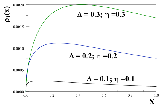
Figure 1: Spectral density for the active-like mode.

It is remarkable that in the absence of other interactions, the propagator of the active-like (lightest) mass eigenstate features a non-vanishing spectral density away from its mass shell for $p^{2}>M^{2}>M^{2}_{1}$. This mode “inherits” a coupling to the continuum “hidden” sector as a consequence of the mixing with the unparticle. The non-vanishing spectral density above the unparticle threshold at $p^{2}=M^{2}$ may lead to opening new kinematic channels when the active-like neutrino is coupled to the standard model fields.

III.2 Complex Poles and Spectral Densities for the Unsterile-like Mode

For $m\ll M$, the self-consistent equation (67) for the unsterile-like mode becomes

$$p^{2}_{2}-M^{2}={2m^{2}}\Big{[}\frac{-p^{2}_{2}+M^{2}-i\epsilon}{\Lambda^{2}}\Big{]}^{\eta}+\cdots$$ (81)

In terms of the dimensionless variables (78) this equation becomes

$$x=\Delta\Big{[}-x-i\epsilon\Big{]}^{\eta}\,.$$ (82)

We find that there is a solution only for

$$\mathrm{Re}(x)>0~{},~{}0\leq\eta<1/3,$$

and it is given by

$$p^{2}_{2}=M^{2}\Big{[}1+\Delta^{\frac{1}{1-\eta}}\,\Big{\{}\cos\Big{(}\frac{\pi\eta}{1-\eta}\Big{)}-i\sin\Big{(}\frac{\pi\eta}{1-\eta}\Big{)}\Big{\}}\Big{]}\,.$$ (83)

This solution describes a pole in the complex plane (a resonance) and near this pole we find

$$\frac{1}{p^{2}-M^{2}_{2}(p)}\approx\frac{Z_{2}}{p^{2}-M^{2}_{2}+iM_{2}\Gamma},$$ (84)

where

$$M^{2}_{2}=M^{2}\Big{[}1+\Delta^{\frac{1}{1-\eta}}\,\cos\Big{(}\frac{\pi\eta}{1-\eta}\Big{)}\Big{]}\;,$$ (85)

$$\Gamma=\frac{M^{2}}{M_{2}}\Delta^{\frac{1}{1-\eta}}\,\sin\Big{(}\frac{\pi\eta}{1-\eta}\Big{)}\;,$$ (86)

and

$$Z_{2}=\frac{1}{1-\eta}\,.$$ (87)

The imaginary part is a consequence of the fact that the real part of the pole is above the unparticle continuum determined by the multiparticle threshold at $p^{2}=M^{2}$. For $F(p)=1$ ($\eta=0$), the largest eigenvalue of the see-saw mass matrix is at $M+m^{2}/M>M$. After mixing, the new pole is in the unparticle continuum, moving off the real axis into a second (or higher) Riemann sheet in the complex $p^{2}$ plane. The imaginary part describes the decay of the unsterile like mode into the active-like mode and particles in the “hidden” conformal sector. A similar phenomenon was observed in the bosonic case in Ref. unparticleus . We refer to $\Gamma$ as the “invisible width” of the unsterile-like neutrino since it describes its decay into an active-like and conformal massless particles in the “hidden sector.” A more detailed discussion and interpretation of this result, based on a renormalization group infradiv ; bogo ; Neubert:2007kh resummation is presented in Sec. III.3.

The spectral density is obtained from the discontinuity across the real axis in the complex $p^{2}$ plane (see Eq.(79))

$$\rho_{2}(x)=\frac{\Theta(x)}{\pi}~{}\frac{\Delta\,x^{\eta}\sin(\pi\eta)}{\Big{[}x-{\Delta}\,x^{\eta}\cos(\pi\eta)\Big{]}^{2}+\Big{[}{\Delta}\,x^{\eta}\sin(\pi\eta)\Big{]}^{2}}\,,$$ (88)

which is displayed in Fig. (2). For $0\leq\eta<1/3$, there is a resonance with a maximum confirmed to be given by

$$x_{p}=\Delta^{\frac{1}{1-\eta}}\,\cos\Big{(}\frac{\pi\eta}{1-\eta}\Big{)},$$ (89)

as obtained in Eq. (85).

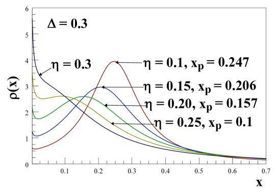
Figure 2: $\rho_{2}(x)$ vs. $x$ for $\Delta=0.3$ and several values of $\eta$. $x_{p}$ is the real part of the complex pole (85,89).

For $\Delta\ll 1$ the real part of the unsterile-like pole is very near the threshold at $p^{2}=M^{2}$ and therefore the dimensionless ratio

$$\frac{\Gamma}{M_{2}-M}\simeq\frac{2\tan\Big{(}\frac{\pi\eta}{1-\eta}\Big{)}}{\Big{[}1+\Delta^{\frac{1}{1-\eta}}\,\cos\Big{(}\frac{\pi\eta}{1-\eta}\Big{)}\Big{]}^{\frac{1}{2}}}$$ (90)

determines if the resonance is broad or narrow as compared to the distance between threshold and the resonance.

For $\eta\ll 1$ ($F(p)\rightarrow 1$), the width becomes very small and the resonance is sharp, centered at the mass of the sterile neutrino $M+m^{2}/M$. As $\eta\rightarrow 1/3$ from below, the real part of the pole approaches threshold ($x_{p}\rightarrow 0$) while the width remains constant. The resonance broadens enormously since the ratio (90) diverges as $\eta\rightarrow 1/3^{-}$, and merges with the threshold at $\eta=1/3$. There are no solutions of the self-consistency condition (81) for a complex pole for $\eta>1/3$.

III.3 Resummation Interpretation of the Decay Width

Consider the unparticle to be a single Dirac fermion (neutrino) interacting with massless particles of the conformal hidden sector, described by a conformal field $\mathcal{A}$. Let us assume such interaction to be of the form

$$\mathcal{L}_{int}=g\,\overline{\Psi}\mathcal{A}\Psi,$$ (91)

where $g$ is a small dimensionless coupling. In perturbation theory, the self-energy of the “unparticle field” $\Psi$ is depicted in Fig. (3)

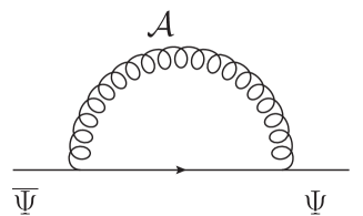
Figure 3: $\Psi$ self-energy to lowest order in g. $\mathcal{A}$ is the conformal field.

To lowest order in g, the self energy, which is once-subtracted to vanish at $\not\!{p}=M$, is given near the mass shell by

$$\Sigma(p)=-\eta(\not\!{p}-M)\,\ln\Bigg{[}\frac{-p^{2}+M^{2}-i\epsilon}{\Lambda^{2}}\Bigg{]},$$ (92)

where $\Lambda$ is a renormalization scale,

$$\eta=cg^{2},$$ (93)

and $c$ is a constant that depends on the nature of the conformal field $\mathcal{A}$ (gauge or scalar massless particle).

Integrating out the conformal field $\mathcal{A}$ leads to the following effective action for $\Psi$

$$\mathcal{L}_{eff} = \overline{\Psi}(\not\!{p}-M)\Bigg{[}1-\eta\ln\Big{(}\frac{-p^{2}+M^{2}-i\epsilon}{\Lambda^{2}}\Big{)}\Bigg{]}\Psi$$ (94)

$$\approx \overline{\Psi}(\not\!{p}-M)\Bigg{[}\frac{-p^{2}+M^{2}-i\epsilon}{\Lambda^{2}}\Bigg{]}^{-\eta}\Psi,$$

where in the last line we have invoked a renormalization group resummation infradiv ; bogo ; Neubert:2007kh of the infrared threshold divergences. The infrared logarithmic divergence at $p^{2}=M^{2}$ and the imaginary part for $p^{2}>M^{2}$ is the result of the emission and absorption of massless quanta, an ubiquitous phenomenon in gauge theories (for a discussion within QCD, see Neubert:2007kh ).

Now consider coupling the heavy neutrino $\Psi$ to a massless (active) neutrino $\psi_{a}$ via the coupling

$$\mathcal{L}_{m}=\overline{\Psi}~{}m~{}\psi_{a}+\mathrm{h.c.}\,,$$ (95)

leading to a see-saw mass matrix of the same form as in Eq. (9) for $F(p)=1$ with $m\ll M$. The see-saw mass matrix can be diagonalized by a unitary transformation with the mixing angle $\theta_{0}$, given by the relations (42). The fields that describe the “mass eigenstates” are

$$\psi_{1} = \cos(\theta_{0})\,\psi_{a}+\sin(\theta_{0})\,\Psi,$$ (96)

$$\psi_{2} = \cos(\theta_{0})\,\Psi-\sin(\theta_{0})\,\psi_{a}\,,$$ (97)

where the masses corresponding to the fields $\psi_{1,2}$ are $M_{1,2}$ respectively, with

$$M_{1}\approx\frac{m^{2}}{M}~{}~{};~{}~{}M_{2}\approx M+\frac{m^{2}}{M}\,.$$ (98)

To lowest order in the see-saw ratio $m/M$, it follows from (42) that

$$\sin(\theta_{0})=\frac{m}{M}\,.$$ (99)

The $\Psi-\psi_{a}$ mixing leads to the following interaction vertex between the fields associated with the mass eigenstates and the conformal field $\mathcal{A}$

$$\mathcal{L}_{int}=g\,\Big{(}\cos(\theta_{0})\overline{\psi}_{2}-\sin(\theta_{0})\overline{\psi}_{1}\Big{)}\mathcal{A}\Big{(}\cos(\theta_{0}){\psi}_{2}-\sin(\theta_{0}){\psi}_{1}\Big{)}.$$ (100)

The self-energy for the $\psi_{2}$ field now includes the diagram depicted in Fig.(4).

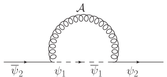
Figure 4: Self-energy for mass eigenstate $\psi_{2}$.

The cut discontinuity across the intermediate state relates the absorptive (imaginary) part of the self-energy on the mass shell of the external fermion to its decay rate. This relation is depicted in Fig. (5).

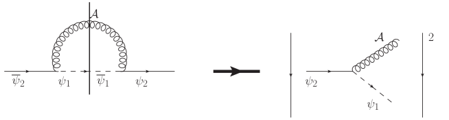
Figure 5: Cutkosky cut for the self-energy for mass eigenstate $\psi_{2}$. The imaginary part of the self-energy determines the width $\Gamma$ in the pole of the propagator.

A standard, straightforward calculation of the decay rate for the process $\psi_{2}\rightarrow\mathcal{A}\,\psi_{1}$, taking $\mathcal{A},\psi_{1}$ to be a massless scalar and Dirac fermion, respectively, yields

$$\Gamma_{\psi_{2}\rightarrow\mathcal{A}\psi_{1}}=2\pi\eta\,M_{2}\,\Big{(}\sin(\theta_{0})\cos(\theta_{0})\Big{)}^{2}\sim\pi\eta\frac{2m^{2}}{M},$$ (101)

where $\eta$ is given by Eq. (93) and we have used the approximations $M_{2}\approx M;$ $\sin(\theta_{0})\approx m/M$ to lowest order in the see-saw ratio $m/M\ll 1$.

This result coincides to lowest order in $\eta$ and $m/M$ with the non-perturbative imaginary part of the unparticle-like pole given by Eq. (86).

This simple analysis confirms that the imaginary part $\Gamma$ in the propagator of the unparticle-like mode (84) describes the decay of the unparticle-like mode into the active-like mode and particles in the hidden conformal sector. This analysis also validates the interpretation of the width of the unsterile mode (resonance) $\Gamma$ given by (86) as an “invisible width” as opposed to the radiative decay width that arises via weak interactions described below.

IV Cosmological consequences: Radiative decay of the unsterile-like neutrino and the X-ray background

Although sterile neutrinos only couple to active neutrinos via an off diagonal mass matrix, the diagonalization of this mass matrix results in effective couplings between the sterile-like neutrino mass eigenstate and standard model particles, namely active neutrinos and charged leptons. Consider the simple case of (canonical) sterile neutrinos coupled to active neutrinos via a see-saw mass matrix of the form (9) with $F=1$, diagonalized by the usual unitary transformation. In this case,

$$\nu_{a} = \cos(\theta_{0})\,\nu_{1}+\sin(\theta_{0})\,\nu_{2}\,,$$ (102)

$$\nu_{s} = \cos(\theta_{0})\,\nu_{2}-\sin(\theta_{0})\,\nu_{1}\,,$$ (103)

where as usual $\nu_{1},\nu_{2}$ are the light (active-like) and heavy (sterile-like) neutrino mass eigenstates, with masses $M_{1}\approx m^{2}/M$; $M_{2}\approx M+m^{2}/M\gg M_{1}$, respectively. The mixing angle is determined by Eqs. (50,48,49) with $F=1$.

The charged current interaction yields an interaction between the sterile-like neutrino and the charged lepton

$$\mathcal{L}_{CC}=g\,\overline{\nu}_{aL}\,\not\!{W}\,l_{L}=g\Big{(}\cos(\theta_{0})\,\overline{\nu}_{1L}+\sin(\theta_{0})\,\overline{\nu}_{2L}\Big{)}\,\not\!{W}\,l_{L}\,.$$ (104)

This interaction vertex leads to the radiative decay of the sterile-like neutrino $\nu_{2}\rightarrow\nu_{1}\,\gamma$ pal . The diagrams that describe this process in unitary gauge are shown in Fig. (6). For $M_{2}\gg M_{1}$, the radiative decay width is given by pal

$$\Gamma_{\nu_{2}\rightarrow\nu_{1}\gamma}\approx\frac{\alpha_{em}}{2}\Big{[}\frac{3G_{F}}{32\pi^{2}}\Big{]}^{2}M^{5}_{2}~{}\Big{[}\frac{m_{l}}{M_{W}}\Big{]}^{4}~{}\sin^{2}(\theta_{0})\,\cos^{2}(\theta_{0})\,,$$ (105)

where $m_{l}$ is the mass of the charged lepton in the loop in Fig. (6).

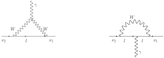
Figure 6: Contributions to radiative decay of a sterile-like neutrino in unitary gauge.

If sterile neutrinos are suitable dark matter candidates, with $M_{2}$ of order of a few keV kusenko ; kusepetra ; micha ; petra ; coldmatter ; boysnudm ; hector ; wu , the radiative decay of the sterile-like neutrino yields a contribution to the X-ray or soft gamma ray background, from which stringent bounds on the mass and mixing angle of the sterile-like neutrino are obtained kusenko ; este ; kuseobs ; micha ; hansen ; dolgov ; aba .

The calculation leading to the radiative decay width (105) uses the standard assumptions, namely that the propagator of $\nu_{2}$ is that of a free particle featuring a single particle pole, that the mixing angles are independent of momentum, and that the in and out states are in their (single particle) mass shells. All of these assumptions must be revised in view of the results obtained in the previous sections. We will proceed to obtain an estimate of the unparticle effects upon the radiative decay width by modifying the calculation leading to (105) by including the following unparticle effects:

• We will consider the mass eigenstate $\nu_{2}$ to be described by the propagator (84) but neglecting the “invisible width” $\Gamma$. This is similar to the situation in calculating the decay of a vector boson by considering it to be an asymptotic state with a propagator featuring a single particle pole. This assumption restricts the validity of our estimate to $0\leq\eta<1/3$ since for $\eta>1/3$, the spectral density of $\nu_{2}$ is a broad continuum above threshold. Furthermore, since the residue at the pole $p^{2}\sim M^{2}_{2}$ is a finite wave function renormalization $Z_{2}$, the total transition probability will be multiplied by $Z_{2}=1/(1-\eta)$. Similarly, the mass eigenstate $\nu_{1}$ is described by the propagator (75), which does feature an isolated single particle pole at $p^{2}=M^{2}_{1}$ but with residue $Z_{1}=1/\big{(}1+\eta\Delta^{2}/2\big{)}$. Therefore, the transition probability must also be multiplied by the wave function renormalization $Z_{1}$.

• The mixing angles $\cos(\theta_{0})\rightarrow\widetilde{c}(p);$ $\sin(\theta_{0})\rightarrow\widetilde{s}(p)$ are given by Eqs. (52,48,49), which depend on the momentum. The radiative decay rate corresponds to setting both the decaying and the product particles on their mass shells. Therefore, $\widetilde{c}(p)$, which is the amplitude of $\nu_{1}$ in $\nu_{a}$, must be evaluated on the mass shell of the active-like mode, namely $p^{2}=M^{2}_{1}$, while $\widetilde{s}(p)$, which is the amplitude of $\nu_{2}$ in $\nu_{a}$, must be evaluated at the mass shell of the unsterile-like mode, $p^{2}=M^{2}_{2}$. Because $M^{2}_{1}$ is below threshold, it follows that $\widetilde{c}(p)$ is real, however, since $M^{2}_{2}$ is above threshold, $\widetilde{s}(p)$ is complex. Being a probability, the decay rate involves the modulus squared of these quantities, namely in the expression (105), we must replace

  $$\cos^{2}(\theta_{0}) \rightarrow \widetilde{c}^{2}(p)=\frac{1}{2}\Big{[}1+\widetilde{\mathcal{C}}(p)\Big{]}_{p^{2}=M^{2}_{1}}\,,$$ (106)

  $$\sin^{2}(\theta_{0}) \rightarrow |\widetilde{s}^{2}(p)|=\frac{1}{2}\Big{|}1-\widetilde{\mathcal{C}}(p)\Big{|}_{p^{2}=M^{2}_{2}}\,.$$ (107)

  For $\eta=0$ ($F(p)=1$) and $m\ll M$, it follows that $\cos(\theta_{0})\approx 1$, $\sin(\theta_{0})\approx m/M$. In the same limit, we find that for $F(p)\neq 1$, $\widetilde{c}(p^{2}=M^{2}_{1})\approx 1$, $\widetilde{s}(p^{2}=M^{2}_{2})\approx m/M\sqrt{F(p^{2}=M^{2}_{2})}$ (see Eqs. (48,49)). The overall change then corresponds to

  $$\cos^{2}(\theta_{0})\sin^{2}(\theta_{0})\rightarrow\frac{1}{\Big{|}F(p)\Big{|}}~{}\cos^{2}(\theta_{0})\sin^{2}(\theta_{0})\,,$$ (108)

  where $p^{2}=p^{2}_{2}$ is given by (83).

Including all of these modifications we obtain the ratio of the radiative decays for the unsterile, and the (canonical) sterile neutrino as

$$\frac{\Gamma^{U}_{\nu_{2}\rightarrow\nu_{1}\gamma}}{\Gamma_{\nu_{2}\rightarrow\nu_{1}\gamma}}=\frac{\Delta^{\frac{\eta}{1-\eta}}~{}\Big{[}\frac{M^{2}}{\Lambda^{2}}\Big{]}^{\eta}}{(1-\eta)\,(1+\eta\frac{\Delta^{2}}{2})}\,.$$ (109)

For a see-saw mass matrix with $m\ll M$, we recognize that

$$\Delta\approx 2\sin^{2}(\theta_{0})\,\Big{[}\frac{M^{2}}{\Lambda^{2}}\Big{]}^{\eta}\,,$$ (110)

where $\theta_{0}$ is the mixing angle for $\eta=0$ (namely the case of canonical sterile neutrinos mixing with active ones). Therefore, we can write the ratio (109) as

$$\frac{\Gamma^{U}_{\nu_{2}\rightarrow\nu_{1}\gamma}}{\Gamma_{\nu_{2}\rightarrow\nu_{1}\gamma}}\sim\frac{\Big{[}2\sin^{2}(\theta_{0})\,\frac{M^{2}}{\Lambda^{2}}\Big{]}^{\frac{\eta}{1-\eta}}}{(1-\eta)\,(1+\eta\frac{\Delta^{2}}{2})}\,.$$ (111)

Taking $\sin\theta\ll 1$ and $M<\Lambda$, consistent with a large see-saw and with the unparticle interpretation of the sterile neutrino below a scale $\Lambda$, respectively, we see that the unparticle nature of the sterile neutrino can lead to a substantial suppression of the radiative decay rate. Even for $\eta\ll 1$, the current bounds on the mixing angles and masses for sterile neutrinos from the observations of the X-ray or soft gamma ray background can be weakened considerably. As an example, taking $\sin(\theta_{0})\sim 10^{-5}$, $M\sim\mathrm{keV}$ and $\Lambda\sim\mathrm{TeV}$, which are within the range of expectation for physics beyond the standard model, and taking $\eta\sim 0.1$ as an example inspired by results in QCD Neubert:2007kh , we find that the ratio (111) $\lesssim\mathcal{O}(10^{-3})$.

This is one of the main cosmological consequences of the unparticle nature of the sterile neutrino.

V Conclusions and further questions

In this article we considered the possibility that the $SU(2)$ singlet sterile neutrino might be an unparticle, an interpolating field that describes a multiparticle continuum as a consequence of coupling to a “hidden” conformal sector and whose correlation functions feature an anomalous scaling dimension $\eta$. We studied the consequences of its mixing with an active neutrino via a see-saw mass matrix. We focused on the simplest setting of one unsterile and one active Dirac neutrino, postponing a more detailed study of Majorana neutrinos and several flavors to further study. Our goals here are two-fold:

1. to study the consequences of the mixing between the non-canonical unsterile with a canonical active neutrino, along with the corresponding dispersion relations and propagating states,

2. to explore cosmological consequences, in particular the radiative decay width of the unsterile-like neutrino into the active-like and a photon, via charged current loops, and to establish how the unparticle nature of the sterile neutrino modifies the radiative line-width, which is an important tool to constrain the mass and mixing angles of cosmologically relevant sterile neutrinos.

We found that the mixing between a non-canonical and a canonical fermion field exhibits several unexpected subtleties. There is no unitary transformation that diagonalizes the full propagator due to the non-canonical nature of the unsterile neutrino. This forces us to make a field redefinition for its complete diagonalization.

The unsterile-like propagating mode is described by a complex pole above the unparticle threshold for $0\leq\eta<1/3$, featuring an “invisible width”. A perturbative analysis and a renormalization group inspired resummation suggest that this width results from the decay of the unsterile-like mode into an active-like mode and particles in the conformal sector. As $\eta\rightarrow 1/3^{-}$, the complex pole merges with the unparticle threshold and disappears, while the spectral density of the unsterile neutrino features a broad continuum above threshold with a threshold enhancement. The active-like mode corresponds to a stable particle, whose propagator features an isolated real pole below the unparticle threshold. This mode “inherits” a non-vanishing spectral density above this threshold, even in the absence of standard model interactions. This novel feature may potentially have relevant consequences since the non-vanishing spectral density may open new kinematic channel for standard model processes even to lowest order in weak interactions, a possibility that will be studied in detail elsewhere.

Considering unsterile neutrino as a dark matter candidate, we studied the influence of the unparticle nature of the sterile neutrino on the radiative decay width into an active neutrino and a photon via charged current loops. We find the ratio of decay widths between the unparticle case and the canonical case to be

$$\frac{\Gamma^{U}_{\nu_{2}\rightarrow\nu_{1}\gamma}}{\Gamma_{\nu_{2}\rightarrow\nu_{1}\gamma}}\approx\frac{\Big{[}2\sin^{2}(\theta_{0})\frac{M^{2}}{\Lambda^{2}}\Big{]}^{\frac{\eta}{1-\eta}}}{(1-\eta)\,(1+\eta\frac{\Delta^{2}}{2})}\,,$$ (112)

where $\theta_{0}$ is the mixing angle for $\eta=0$, $M$ is approximately the mass of the unsterile like neutrino and $\Lambda\gg M$ is the unparticle scale. This ratio suggests a substantial suppression of the radiative decay line width for $M\sim\mathrm{keV}$ and $\Lambda\sim\mathrm{TeV}$, even for $\eta\lesssim 0.1$. This results in a weakening of the bounds on the mass and mixing angle from the X-ray and soft gamma ray backgrounds.

Of course, a detailed assessment of the suppression of the radiative decay width hinges on the (unknown) values of $\Lambda$ and $\eta$, which may emerge from the experimental program at LHC in the exploration of physics beyond the standard model.

To further explore the possibility of an unsterile neutrino as a dark matter candidate, understanding its production process is necessary. Since an unsterile neutrino only interacts directly with the active one, the most effective dark matter production mechanism in this scenario is via unsterile-active neutrino oscillations. It would be interesting to study the implications of our results in Section III in the dark matter production mechanism along the line of Ref. dw .

Appendix A An Alternative Explanation for the Non-unitary Transformation

In the helicity basis of Eq. (28), the Lagrangian density in momentum space is given by

$${\cal L}=\sum_{h}\left(\begin{array}[]{cc}{\xi_{R}^{h}}^{\dagger}(-p)&{\xi_{L}^{h}}^{\dagger}(-p)\end{array}\right)\,\left(\begin{array}[]{cc}(p^{0}-h|\vec{p}|)\mathds{F}&\mathds{M}\\ \mathds{M}&(p^{0}+h|\vec{p}|)\mathds{F}\end{array}\right)\,\left(\begin{array}[]{c}\xi_{R}^{h}(p)\\ \xi_{L}^{h}(p)\end{array}\right).$$ (113)

Lorentz invariance does not allow us to mix the $(2,1)$-representation of the Lorentz group with the $(1,2)$-representation. Therefore, to diagonalize the action, the allowed transformation is $\xi_{R,L}^{h}\rightarrow{\cal U}_{R,L}\,\xi_{R,L}^{h}$, such that all the following matrices:

$${\cal U}_{R}\,\Big{[}(p^{0}-h|\vec{p}|)\mathds{F}\Big{]}\,{\cal U}_{R}^{-1},~{}~{}{\cal U}_{L}\,\Big{[}(p^{0}+h|\vec{p}|)\mathds{F}\Big{]}\,{\cal U}_{L}^{-1},~{}~{}{\cal U}_{R}\;\mathds{M}\;{\cal U}_{L}^{-1}~{}~{}{\rm and}~{}~{}{\cal U}_{L}\;\mathds{M}\;{\cal U}_{R}^{-1}$$ (114)

are all diagonal. Since $\mathds{F}$ is diagonal, and yet not proportional to the identity, the only possible unitary transformations that diagonalize the first two are

$${\cal U}_{R,L}=\left(\begin{array}[]{cc}1&0\\ 0&\pm\,1\end{array}\right)~{}~{}{\rm or}~{}~{}\left(\begin{array}[]{cc}\pm\,1&0\\ 0&1\end{array}\right).$$ (115)

However, none of the combinations of these possibilities diagonalize the last two matrices in (114). Therefore, there is no unitary transformation that diagonalizes the full propagator.

References

- (1) For a thorough description of the see-saw mechanism and list of references see Massive neutrinos in physics and astrophysics, R. N. Mohapatra, P. B. Pal, (World Scientific, Singapore, 1997).
- (2) S. Dodelson and L. M. Widrow, Phys. Rev. Lett. 72, 17 (1994) [arXiv:hep-ph/9303287].
- (3) S. Colombi, S. Dodelson and L. M. Widrow, Astrophys. J. 458, 1 (1996) [arXiv:astro-ph/9505029].
- (4) X. D. Shi and G. M. Fuller, Phys. Rev. Lett. 82, 2832 (1999) [arXiv:astro-ph/9810076]; K. Abazajian, G. M. Fuller and M. Patel, Phys. Rev. D 64, 023501 (2001) [arXiv:astro-ph/0101524]; K. N. Abazajian and G. M. Fuller, Phys. Rev. D 66, 023526 (2002) [arXiv:astro-ph/0204293]; G. M. Fuller, A. Kusenko, I. Mocioiu and S. Pascoli, Phys. Rev. D 68, 103002 (2003) [arXiv:astro-ph/0307267]; K. Abazajian, Phys. Rev. D 73, 063513 (2006) [arXiv:astro-ph/0512631].
- (5) M. Shaposhnikov and I. Tkachev, Phys. Lett. B 639, 414 (2006) [arXiv:hep-ph/0604236]; M. Shaposhnikov, JHEP 0808, 008 (2008) [arXiv:0804.4542 [hep-ph]], arXiv:astro-ph/0703673.
- (6) A. Kusenko, AIP Conf. Proc. 917, 58 (2007) [arXiv:hep-ph/0703116], Int. J. Mod. Phys. D 16, 2325 (2007) [arXiv:astro-ph/0608096]; T. Asaka, M. Shaposhnikov and A. Kusenko, Phys. Lett. B 638, 401 (2006) [arXiv:hep-ph/0602150]; P. L. Biermann and A. Kusenko, Phys. Rev. Lett. 96, 091301 (2006) [arXiv:astro-ph/0601004].
- (7) K. Petraki and A. Kusenko, Phys. Rev. D 77, 065014 (2008) [arXiv:0711.4646 [hep-ph]].
- (8) K. Petraki, Phys. Rev. D 77, 105004 (2008) [arXiv:0801.3470 [hep-ph]].
- (9) D. Boyanovsky, H. J. de Vega and N. Sanchez, Phys. Rev. D 77, 043518 (2008) [arXiv:0710.5180 [astro-ph]].
- (10) A. Boyarsky, J. W. den Herder, A. Neronov and O. Ruchayskiy, Astropart. Phys. 28, 303 (2007) [arXiv:astro-ph/0612219], A. Boyarsky, D. Iakubovskyi, O. Ruchayskiy and V. Savchenko, Mon. Not. Roy. Astron. Soc. 387, 1361 (2008) [arXiv:0709.2301 [astro-ph]], A. Boyarsky, D. Malyshev, A. Neronov and O. Ruchayskiy, Mon. Not. Roy. Astron. Soc. 387, 1345 (2008) [arXiv:0710.4922 [astro-ph]], A. Boyarsky, O. Ruchayskiy and M. Shaposhnikov, arXiv:0901.0011 [hep-ph].
- (11) D. Boyanovsky, Phys. Rev. D 78, 103505 (2008) [arXiv:0807.0646 [astro-ph]].
- (12) M. Loewenstein, A. Kusenko and P. L. Biermann, arXiv:0812.2710 [astro-ph].
- (13) H. J. de Vega and N. G. Sanchez, arXiv:0901.0922 [astro-ph.CO].
- (14) J. Wu, C. M. Ho and D. Boyanovsky, arXiv:0902.4278 [hep-ph].
- (15) P. B. Pal and L. Wolfenstein, Phys. Rev. D 25, 766 (1982).
- (16) A. D. Dolgov and S. H. Hansen, Astroparticle Physics 16, 339, (2002) arXiv:hep-ph/0103118.
- (17) S. Riemer-Sorensen, S. H. Hansen and K. Pedersen, Astrophys. J. 644, L33 (2006) [arXiv:astro-ph/0603661]; S. Riemer-Sorensen, K. Pedersen, S. H. Hansen and H. Dahle, Phys. Rev. D 76, 043524 (2007) [arXiv:astro-ph/0610034].
- (18) . N. Abazajian, M. Markevitch, S. M. Koushiappas and R. C. Hickox, Phys. Rev. D 75, 063511 (2007) [arXiv:astro-ph/0611144].
- (19) S. Riemer-Sorensen and S. H. Hansen, arXiv:0901.2569 [astro-ph].
- (20) V. G. Sinitsyna, M. Masip, S. I. Nikolsky and V. Y. Sinitsyna, arXiv:0903.4654 [hep-ph].
- (21) A. A. Aguilar-Arevalo et al. [The MiniBooNE Collaboration], Phys. Rev. Lett. 98, 231801 (2007) [arXiv:0704.1500 [hep-ex]].
- (22) M. Maltoni and T. Schwetz, Phys. Rev. D 76, 093005 (2007) [arXiv:0705.0107 [hep-ph]].
- (23) S. N. Gninenko, arXiv:0902.3802 [hep-ph].
- (24) H. Georgi, Phys. Rev. Lett. 98, 221601 (2007) [arXiv:hep-ph/0703260]; H. Georgi, Phys. Lett. B 650, 275 (2007) [arXiv:0704.2457 [hep-ph]].
- (25) K. Cheung, W. Y. Keung and T. C. Yuan, Phys. Rev. Lett. 99, 051803 (2007) [arXiv:0704.2588 [hep-ph]]; A. Arhrib, K. Cheung, C. W. Chiang and T. C. Yuan, Phys. Rev. D 73, 075015 (2006) [arXiv:hep-ph/0602175]; for a recent review see: K. Cheung, W. Y. Keung and T. C. Yuan, AIP Conf. Proc. 1078, 156 (2009) [arXiv:0809.0995 [hep-ph]].
- (26) J. L. Feng, A. Rajaraman and H. Tu, Phys. Rev. D 77, 075007 (2008) [arXiv:0801.1534 [hep-ph]]; A. Rajaraman, AIP Conf. Proc. 1078, 63 (2009) [arXiv:0809.5092 [hep-ph]].
- (27) A. Delgado, J. R. Espinosa and M. Quiros, JHEP 0710, 094 (2007) [arXiv:0707.4309 [hep-ph]]; A. Delgado, J. R. Espinosa, J. M. No and M. Quiros, Phys. Rev. D 79, 055011 (2009) [arXiv:0812.1170 [hep-ph]].
- (28) T. Banks and A. Zaks, Nucl. Phys. B 196, 189 (1982).
- (29) P. J. Fox, A. Rajaraman and Y. Shirman, Phys. Rev. D 76, 075004 (2007) [arXiv:0705.3092 [hep-ph]].
- (30) M. Luo and G. Zhu, Phys. Lett. B 659, 341 (2008) [arXiv:0704.3532 [hep-ph]]; Y. Liao, Phys. Lett. B 665, 356 (2008) [arXiv:0804.0752 [hep-ph]]; R. Basu, D. Choudhury and H. S. Mani, arXiv:0803.4110 [hep-ph].
- (31) B. Grinstein, K. A. Intriligator and I. Z. Rothstein, Phys. Lett. B 662, 367 (2008) [arXiv:0801.1140 [hep-ph]].
- (32) Y. Liao and J. Y. Liu, Phys. Rev. Lett. 99, 191804 (2007) [arXiv:0706.1284 [hep-ph]].
- (33) S. Hannestad, G. Raffelt and Y. Y. Y. Wong, Phys. Rev. D 76, 121701 (2007) [arXiv:0708.1404 [hep-ph]].
- (34) N. G. Deshpande, S. D. H. Hsu and J. Jiang, Phys. Lett. B 659, 888 (2008) [arXiv:0708.2735 [hep-ph]].
- (35) A. Freitas and D. Wyler, JHEP 0712, 033 (2007) [arXiv:0708.4339 [hep-ph]].
- (36) J. McDonald, arXiv:0805.1888 [hep-ph]; JCAP 0903, 019 (2009) [arXiv:0709.2350 [hep-ph]].
- (37) H. Davoudiasl, Phys. Rev. Lett. 99, 141301 (2007) [arXiv:0705.3636 [hep-ph]].
- (38) I. Lewis, arXiv:0710.4147 [hep-ph].
- (39) G. L. Alberghi, A. Y. Kamenshchik, A. Tronconi, G. P. Vacca and G. Venturi, Phys. Lett. B 662, 66 (2008) [arXiv:0710.4275 [hep-th]].
- (40) S. L. Chen, X. G. He, X. P. Hu and Y. Liao, Eur. Phys. J. C 60, 317 (2009) [arXiv:0710.5129 [hep-ph]].
- (41) T. Kikuchi and N. Okada, Phys. Lett. B 665, 186 (2008) [arXiv:0711.1506 [hep-ph]].
- (42) Y. Gong and X. Chen, Eur. Phys. J. C 57, 785 (2008) [arXiv:0803.3223 [astro-ph]].
- (43) H. Collins and R. Holman, Phys. Rev. D 78, 025023 (2008) [arXiv:0802.4416 [hep-ph]].
- (44) D. C. Dai and D. Stojkovic, arXiv:0812.3396 [gr-qc].
- (45) R. Zwicky, J. Phys. Conf. Ser. 110, 072050 (2008) [arXiv:0710.4430 [hep-ph]].
- (46) Y. f. Wu and D. X. Zhang, arXiv:0712.3923 [hep-ph]; R. Mohanta and A. K. Giri, Phys. Rev. D 76, 057701 (2007) [arXiv:0707.3308 [hep-ph]]; J. K. Parry, arXiv:0810.0971 [hep-ph].
- (47) G. J. Ding and M. L. Yan, Phys. Rev. D 78, 075015 (2008) [arXiv:0706.0325 [hep-ph]]; G. Bhattacharyya, D. Choudhury and D. K. Ghosh, Phys. Lett. B 655, 261 (2007) [arXiv:0708.2835 [hep-ph]].
- (48) D. Boyanovsky, R. Holman and J. A. Hutasoit, Phys. Rev. D 79, 085018 (2009) [arXiv:0812.4723 [hep-ph]].
- (49) M. A. Stephanov, Phys. Rev. D 76, 035008 (2007) [arXiv:0705.3049 [hep-ph]].
- (50) D. Amit, Field Theory, the Renormalization Group and Critical Phenomena (McGraw-Hill, N.Y. 1978).
- (51) E. Brezin, J. C. Le Guillou, J. Zinn-Justin, in Phase Transitions and Critical Phenomena, Vol. 6 (Ed. C. Domb, M. S. Green, Academic Press, London, 1976) (page 127).
- (52) M. Neubert, Phys. Lett. B 660, 592 (2008) [arXiv:0708.0036 [hep-ph]].
- (53) F. Bloch and A. Nordsieck, Phys. Rev. 52, 54 (1937).
- (54) N.N.Bogoliubov, D.V.Shirkov, Introduction to the theory of quantized fields, (Interscience Publishers, N.Y. 1959).
- (55) D. Boyanovsky and H. J. de Vega, Annals Phys. 307, 335 (2003) [arXiv:hep-ph/0302055].
- (56) X. Q. Li, Y. Liu and Z. T. Wei, Eur. Phys. J. C 56, 97 (2008) [arXiv:0707.2285 [hep-ph]].
- (57) S. Zhou, Phys. Lett. B 659, 336 (2008) [arXiv:0706.0302 [hep-ph]].
- (58) G. Gonzalez-Sprinberg, R. Martinez and O. A. Sampayo, Phys. Rev. D 79, 053005 (2009) [arXiv:0808.1747 [hep-ph]].
- (59) G. Cacciapaglia, G. Marandella and J. Terning, JHEP 0902, 049 (2009) [arXiv:0804.0424 [hep-ph]].
- (60) G. von Gersdorff and M. Quiros, arXiv:0901.0006 [hep-ph].
- (61) T. Schwetz, JHEP 0802, 011 (2008) [arXiv:0710.2985 [hep-ph]].
- (62) Q. Duret, B. Machet and M. I. Vysotsky, Mod. Phys. Lett. A 24, 273 (2009) [arXiv:0810.4449 [hep-ph]]; arXiv:0805.4121 [hep-ph].
- (63) J. P. Silva, Phys. Rev. D 62, 116008 (2000) [arXiv:hep-ph/0007075]; G. C. Branco, L. Lavoura, J. P. Silva, CP Violation, (Oxford University Press, Oxford, U.K., 1999).
- (64) M. Beuthe, G. Lopez Castro and J. Pestieau, Int. J. Mod. Phys. A 13, 3587 (1998) [arXiv:hep-ph/9707369].
- (65) L. Alvarez-Gaume, C. Kounnas, S. Lola and P. Pavlopoulos, Phys. Lett. B 458, 347 (1999) [arXiv:hep-ph/9812326].