A Simple Sequential Spectrum Sensing Scheme for Cognitive Radio

Abstract

Cognitive radio that supports a secondary and opportunistic access to licensed spectrum shows great potential to dramatically improve spectrum utilization. Spectrum sensing performed by secondary users to detect unoccupied spectrum bands, is a key enabling technique for cognitive radio. This paper proposes a truncated sequential spectrum sensing scheme, namely the sequential shifted chi-square test (SSCT). The SSCT has a simple test statistic and does not rely on any deterministic knowledge about primary signals. As figures of merit, the exact false-alarm probability is derived, and the miss-detection probability as well as the average sample number (ASN) are evaluated by using a numerical integration algorithm. Corroborating numerical examples show that, in comparison with fixed-sample size detection schemes such as energy detection, the SSCT delivers considerable reduction on the ASN while maintaining a comparable detection performance.

I Introduction

Most radio frequency spectrum is allocated primarily based on fixed spectrum allocation strategies that grant licensed users to exclusively use specific frequency bands to avoid interference. Recent reports [1] released by the Federal Communications Commission show that, a large amount of allocated spectrum particularly television bands, is substantially under-utilized most of the time whereas a small portion of spectrum bands such as cellular bands, experience increasingly congestion and scarcity due to rapid deployment of various wireless services. Cognitive radio, which enables secondary (unlicensed) users to access licensed spectrum bands not being currently occupied, can fundamentally alter this unbalanced spectrum usage and therefore can dramatically improve spectrum utilization. Since licensed (primary) users are prior to unlicensed (secondary) users in utilizing spectrum, the secondary and opportunistic access to licensed spectrum bands is only allowed to have negligible probability of deteriorating the quality of service (QoS) of primary users (PUs). Spectrum sensing performed by secondary users (SUs) to detect the unoccupied frequency bands, is the key enabling technique to meet this requirement, thereby receiving considerable amount of research interest recently [2, 3, 4, 5].

Albeit in essence a conventional signal detection problem, the design of a spectrum sensing scheme needs to cope with several critical challenges that stem from special attributes of cognitive radio networks. First, it is often difficult for SUs in a cognitive radio network to acquire complete or even partial knowledge about primary signals. Secondly, SUs need to be able to quickly detect primary signals at a fairly low detection signal-to-noise ratio (SNR) level with low detection error probabilities. To this end, several spectrum sensing schemes, such as matched-filter detection [6], energy detection [2, 7], and cyclostationary detection [8], have been proposed and investigated. Among these sensing schemes, energy detection is particularly appealing as it does not rely on any deterministic knowledge of the primary signals and has low implementation complexity. However, when the detection SNR is low, energy detection entails a large amount of sensing time to ensure high detection accuracy, e.g., the sensing time is inversely proportional to the square of SNR [9]. To overcome this shortcoming, several sensing schemes based on the sequential probability ratio test (SPRT) have been proposed under various cognitive radio settings [10, 11, 4].

The SPRT has been widely used in many scientific and engineering fields since it was introduced by Wald [12] in 1940s . Perhaps, the most remarkable character of the SPRT is that, for given detection error probabilities, the SPRT requires the smallest average sample number (ASN) for testing simple hypotheses [13]. In comparison to fixed-sample-size sensing schemes, the sensing scheme based on the SPRT requires much reduced sensing time on the average while maintaining the same detection performance [10]. Nonetheless, the existing SPRT based sensing scheme [10] suffers from several potential drawbacks. First, when primary signals are taken from a finite alphabet, the test statistic involves a special function, which incurs high implementation complexity [10, 4]. Second, evaluating the probability ratio requires deterministic knowledge or statistical distribution of certain parameters of the primary signals. Acquiring such deterministic information or statistical distribution is practically difficult in general. Thirdly, the existing SPRT based sensing scheme adopts the Wald’s choice on the thresholds [12]. However, the Wald’s choice, which works well for the non-truncated SPRT, increases error probabilities when applied to the truncated SPRT.

In this paper, we propose a truncated sequential spectrum sensing scheme, namely the sequential shifted chi-square test (SSCT). The SSCT possesses several attractive features: 1) Like energy detection, the SSCT only requires the knowledge on noise power and does not rely on any deterministic knowledge about primary signals; 2) compared to fixed-sample-size detection such as energy detection, the SSCT is capable of delivering considerable reduction on the average sensing time while maintaining a comparable detection performance; 3) in comparison with the SPRT based sensing scheme [10], the SSCT has a much simpler test statistic and thus has lower implementation complexity; 4) and the SSCT offers desirable flexibility to strike a trade-off between detection performance and sensing time when the operating SNR is higher than the minimum detection SNR. To evaluate the detection performance of the SSCT, we derive the exact false-alarm probability, and employ a numerical integration algorithm from [14] to compute the miss-detection probability and the ASN in a recursive manner. Notably, the problem of evaluating the false-alarm probability of the SSCT resembles the exact operating characteristic (OC) evaluation problem associated with truncated sequential life tests involving the exponential distribution [15][16]. The latter problem has been solved by Woodall and Kurkjian [15]. Despite the similarity of these two problems, the Woodall-Kurkjian approach cannot be applied to directly evaluate the false-alarm probability of the SSCT. In addition, the Woodall-Kurkjian approach is not applicable to evaluate the ASN for truncated sequential life tests involving exponential distribution [16]. As a byproduct, our approach to evaluating the false-alarm probability of the SSCT, can be readily modified to evaluate the ASN for truncated sequential life tests in the exponential case.

The remainder of this paper is organized as follows. Section II presents the problem formulation and provides necessary preliminaries on energy detection and a SPRT based sensing scheme. Section III introduces the SSCT and its equivalent test procedure. Section IV deals with the evaluation of the error probabilities of the SSCT. In particular, this section provides an exact result for the false-alarm probability, and a numerical integration algorithm to recursively compute the miss-detection probability. Section V presents an evaluation result on the ASN of the SSCT, while Section VI provides several numerical examples. Finally, Section VII concludes the paper.

The following notation is used in this paper. Boldface upper and lower case letters are used to denote matrices and vectors, respectively; ${\mbox{\boldmath$I$}}_{k}$ denotes a $k\times k$ identity matrix; $E[\cdot]$ denotes the expectation operator. $(\cdot)^{T}$ denotes the transpose operation; ${\mathbf{1}}_{k}$ denotes a $k\times 1$ vector whose entries are all ones; $\aleph_{p}^{q}$ denotes a set of consecutive integers from $p$ to $q$, i.e., $\aleph_{p}^{q}:=\{p,p+1,\ldots,q\}$, where $p$ is a non-negative integer and $q$ is a positive integer or infinity; $(\cdot)^{c}$ denotes a complement of a set; ${\mathbb{I}}_{\{x\geq t\}}$ denotes an indicator function defined as ${\mathbb{I}}_{\{x\geq t\}}=1$ if $x\geq t$ and ${\mathbb{I}}_{\{x\geq t\}}=0$ if $x<t$, where $x$ is a variable and $t$ is a constant.

II Problem Formulation and Preliminaries

In this section, we start by presenting a statistical formulation of the spectrum sensing problem for a single SU cognitive radio system. We next give a brief overview on two sensing schemes, energy detection and a SPRT based sensing scheme, which are closely related to the SSCT.

II-A Problem Formulation

Consider a narrow-band cognitive radio communication system having a single SU. The SU shares the same spectrum with a single PU and needs to detect the presence/absence of the PU. Let $H_{0}$ and $H_{1}$ denote the null and alternative hypotheses, respectively. The detection of the primary signals can be formulated as a binary hypothesis testing problem as follows

$$H_{0}:r_{i}=w_{i},~{}i=1,2,\ldots,$$ (1)

$$H_{1}:r_{i}=hs_{i}+w_{i},~{}i=1,2,\ldots,$$ (2)

where $r_{i}$ is the received signal at the SU, $w_{i}$ is additive white Gaussian noise, $h$ is the channel gain between the PU and the SU, and $s_{i}$ is the transmitted signal of the PU. We further assume that

1. $w_{i}$’s are modeled as independent and identically distributed (i.i.d.) zero mean complex Gaussian random variables (RVs) with variance $\sigma_{w}^{2}/2$ per dimension, i.e., $w_{i}\sim\mathcal{CN}(0,\sigma_{w}^{2})$,

2. the channel gain $h$ is constant during the sensing period,

3. the primary signal samples $s_{i}$ are i.i.d.,

4. $w_{i}$ and $s_{i}$ are statistically independent,

5. and the perfect knowledge on the noise variance (noise power) $\sigma_{w}^{2}$ is available at the SU.

II-B Preliminaries

II-B1 Energy Detection

In energy detection, the energy of the received signal samples is first computed and then is compared to a predetermined threshold. The test procedure of energy detection is given as

$$T({\mbox{\boldmath$r$}})=\sum_{i=1}^{M}|r_{i}|^{2}\underset{H_{0}}{\overset{H_{1}}{\gtreqqless}}\gamma_{\text{ed}}$$

where ${\mbox{\boldmath$r$}}:=[r_{1},r_{2},\ldots,r_{M}]$, $T({\mbox{\boldmath$r$}})$ denotes the test statistic, $M$ denotes the fixed sample size, and $\gamma_{\text{ed}}$ denotes a threshold for energy detection.

Recall that $w_{i}$ is a zero mean complex Gaussian RV with variance $\sigma_{w}^{2}/2$ per dimension. Under $H_{0}$, the RV $2T({\mbox{\boldmath$r$}})/\sigma_{w}^{2}$ is a central chi-square RV with $2M$ degrees of freedom whereas under $H_{1}$, the RV $2T({\mbox{\boldmath$r$}})/\sigma_{w}^{2}$ conditioning on $|s_{i}|^{2}~{},i=1,\ldots,M$, is a noncentral chi-square RV with $2M$ degrees of freedom and non-centrality parameter $2|h|^{2}\sum_{i=1}^{M}|s_{i}|^{2}/\sigma_{w}^{2}$. As $M$ increases, $2|h|^{2}\sum_{i=1}^{M}|s_{i}|^{2}/\sigma_{w}^{2}$ approaches $2M|h|^{2}\sigma_{s}^{2}/\sigma_{w}^{2}$, where $\sigma_{s}^{2}$ denotes the average symbol energy. Let us define ${\tt{SNR}}_{m}:=|h|^{2}\sigma_{s}^{2}/\sigma_{w}^{2}$ as the minimum detection SNR. Notice that the minimum detection ${\tt{SNR}}_{m}$ is a design parameter referring to the minimum SNR value by which a detector can achieve the target false-alarm and miss-detection probabilities. In practice, it is highly likely that ${\tt{SNR}}_{m}$ is different from the exact operating SNR, which is typically difficult to acquire in practice. To distinguish these two different SNRs, we denote by ${\tt{SNR}}_{o}$ the operating SNR.

It follows directly from the central limit theorem (CLT) that as $M$ approaches infinity, the distribution of $2T({\mbox{\boldmath$r$}})/\sigma_{w}^{2}$ converges to a normal distribution given as follows [3]

$$\frac{2T({\mbox{\boldmath$r$}})}{\sigma_{w}^{2}}\sim\begin{cases}\mathcal{N}(2M,4M),&\text{under}~{}H_{0},\\ \mathcal{N}\big{(}2M(1+{\tt{SNR}}_{m}),4M(1+2{\tt{SNR}}_{m})\big{)},&\text{under}~{}H_{1}.\end{cases}$$ (3)

Typically, the required sample size $M$ is determined by the target false-alarm and miss-detection probabilities, which we denote by $\bar{\alpha}_{\text{ed}}$ and $\bar{\beta}_{\text{ed}}$ respectively. Let $M_{\text{ed}}^{\min}$ be the minimum sample number required to achieve the target $\bar{\alpha}_{\text{ed}}$ and $\bar{\beta}_{\text{ed}}$ at the detection ${\tt{SNR}}_{m}$ level. As shown in [2], we have

$$M_{\text{ed}}^{\min}={\tt{Ceil}}\Big{(}({\tt{SNR}}_{m})^{-2}\Big{[}\mathcal{Q}^{-1}(\bar{\alpha}_{\text{ed}})-\mathcal{Q}^{-1}(1-\bar{\beta}_{\text{ed}})\sqrt{2{\tt{SNR}}_{m}+1}\Big{]}^{2}\Big{)}=O({\tt{SNR}}_{m}^{-2})$$ (4)

where ${\tt{Ceil}}(x)$ denotes the smallest integer not less than $x$, $\mathcal{Q}(\cdot)$ is the complementary cumulative distribution function of the standard normal RV, i.e., $\mathcal{Q}(x):=(2\pi)^{-1/2}\int_{x}^{\infty}e^{-t^{2}/2}dt$, and $\mathcal{Q}^{-1}(\cdot)$ denotes its inverse function. It is evident from (4) that for energy detection, the number of the required sensing samples is inversely proportional to ${\tt{SNR}}_{m}^{2}$ when ${\tt{SNR}}_{m}$ is sufficiently small [9].

As clear from the above description, energy detection has a simple test statistic and has low implementation complexity [7]. In addition, known as a form of non-coherent detection, energy detection only requires the knowledge on noise power and does not rely on any deterministic knowledge about the primary signals $s_{i}$. However, one major drawback of energy detection is that, at a low detection SNR level, it requires a large amount of sensing time to achieve low detection error probabilities.

II-B2 A SPRT Based Sensing Scheme

In comparison with a fixed-sample-size detection such as energy detection, the SPRT is capable of achieving the same detection performance with a much reduced ASN [13]. We next investigate a SPRT based sensing scheme that relies on the amplitude squares of the received signal samples [4, 10]. To simplify our description, we now assume that the amplitude squares of primary signals, $|s_{i}|^{2},~{}i=1,2,\ldots$, are perfectly known at the SU. With this assumption, the spectrum sensing problem formulated in (1) becomes a simple hypothesis testing problem, which is the original setting considered by Wald [12].

We normalize $|r_{i}|^{2}$ as $v_{i}:=2|r_{i}|^{2}/\sigma_{w}^{2}$ for the convenience of derivation. Note that under $H_{0}$, $v_{i}$ is an exponential RV with rate parameter $1/2$ and under $H_{1}$, $v_{i}$ conditional on $|s_{i}|^{2}$ is a noncentral chi-square RV with two degrees of freedom and non-centrality parameter $\lambda_{i}$ that can be readily obtained as $\lambda_{i}=2|h|^{2}|s_{i}|^{2}/\sigma_{w}^{2}$. Hence, the probability density function (PDF) of $v_{i}$ under $H_{0}$ is

$$p_{H_{0}}(v_{i})=\frac{1}{2}e^{-v_{i}/2}$$ (5)

whereas under $H_{1}$, the PDF of $v_{i}$ conditional on $\lambda_{i}$ is

$$p_{H_{1}}(v_{i}|\lambda_{i})=\frac{1}{2}e^{-(v_{i}+\lambda_{i})/2}I_{0}(\sqrt{\lambda_{i}v_{i}})$$ (6)

where $I_{0}(\cdot)$ is the zeroth-order modified Bessel function of the first kind. After collecting $N$ samples, we can express the accumulative log-likelihood ratio as

$$L_{N}({\mbox{\boldmath$v$}}_{N}|\boldsymbol{\lambda}_{N}) =\log\frac{p_{{\mbox{\boldmath$v$}}|H_{1}}({\mbox{\boldmath$v$}}_{N}|\boldsymbol{\lambda}_{N})}{p_{{\mbox{\boldmath$v$}}|H_{0}}({\mbox{\boldmath$v$}}_{N})}=\sum_{i=1}^{N}z_{i}=-\sum_{i=1}^{N}\lambda_{i}/2+\sum_{i=1}^{N}\log I_{0}(\sqrt{\lambda_{i}v_{i}})$$ (7)

where ${\mbox{\boldmath$v$}}_{N}:=(v_{1},v_{2},\ldots,v_{N})$, $z_{i}=\log\big{(}p_{H_{1}}(v_{i}|\lambda_{i})/p_{H_{0}}(v_{i})\big{)}$, and $\boldsymbol{\lambda}_{N}:=(\lambda_{1},\lambda_{2},\ldots,\lambda_{N})$. The test procedure is given as follows: Reject $H_{0}$, if $L_{N}({\mbox{\boldmath$v$}}_{N}|\boldsymbol{\lambda}_{N})\geq b_{L}$; Accept $H_{0}$, if $L_{N}({\mbox{\boldmath$v$}}_{N}|\boldsymbol{\lambda}_{N})\leq a_{L}$; and continue sensing, if $a_{L}<L_{N}({\mbox{\boldmath$v$}}_{N}|\boldsymbol{\lambda}_{N})<b_{L}$. In [12], Wald specified a particular choice of the thresholds $a_{L}$ and $b_{L}$ for the non-truncated SPRT as follows

$$a_{L}=\log\frac{\bar{\beta}_{\text{sprt}}}{1-\bar{\alpha}_{\text{sprt}}},~{}\text{and}\quad b_{L}=\log\frac{1-\bar{\beta}_{\text{sprt}}}{\bar{\alpha}_{\text{sprt}}}$$ (8)

where $\bar{\alpha}_{\text{sprt}}$ and $\bar{\beta}_{\text{sprt}}$ denote the target false-alarm and miss-detection probabilities, respectively. For a non-truncated SPRT, the Wald’s choice on $a_{L}$ and $b_{L}$ yields true false-alarm and miss-detection probabilities that are fairly close to the target ones.

Let $z$ be a RV that has the same PDF as $z_{i}$. It has been pointed out in [17] that, in the SPRT, if hypotheses $H_{0}$ and $H_{1}$ are distinct, then $E_{H_{0}}(z)<0<E_{H_{1}}(z)$, where $E_{H_{i}}(\cdot)$ denotes the conditional expectation under $H_{i},~{}i=1,2$.

As evident from (7), one shortcoming of this SPRT-based sensing scheme is that the test statistic contains a modified Bessel function, which may result in high implementation complexity. When the perfect knowledge of the instantaneous amplitude squares of the primary signals is not available, the PDF under $H_{1}$ is not completely known, i.e., the alternative hypothesis is composite. Generally speaking, two approaches, the Bayesian approach or the generalized likelihood ratio test, can be used to deal with such a case. In the Bayesian approach, a prior PDF of the amplitude squares of the primary signals is required and multiple summations over all possible amplitudes of the primary signals need to be performed, whereas in the generalized likelihood ratio test, a maximum likelihood estimation (MLE) of the amplitude squares of the primary signals is needed [18]. Either of these two approaches, however, leads to a considerable increase in implementation complexity.

III A Simple Sequential Spectrum Sensing Scheme

We now present a simple sequential spectrum sensing scheme with the following test statistic

$$\Lambda_{N}=\sum_{i=1}^{N}\left(|r_{i}|^{2}-\Delta\right)$$ (9)

where $\Delta$ is a predetermined constant. Assuming that the detector needs to make a decision within $M$ samples, we propose the following test procedure

$$\mathtt{Reject}~{}H_{0}:~{} \text{if}~{}\Lambda_{N}\geq b~{}\text{and}~{}N\leq M-1,~{}\text{or~{}if}~{}\Lambda_{M}\geq\gamma;$$ (10)

$$\mathtt{Accept}~{}H_{0}:~{} \text{if}~{}\Lambda_{N}\leq a~{}\text{and}~{}N\leq M-1,~{}\text{or~{}if}~{}\Lambda_{M}<\gamma;~{}$$ (11)

$$\mathtt{Continue~{}Sensing:}~{} \text{if}~{}\Lambda_{N}\in(a,b)~{}\text{and}~{}N\leq M-1$$ (12)

where $a$, $b$, and $\gamma$ are three predetermined thresholds with $a<0$, $b>0$, and $\gamma\in(a,b)$.

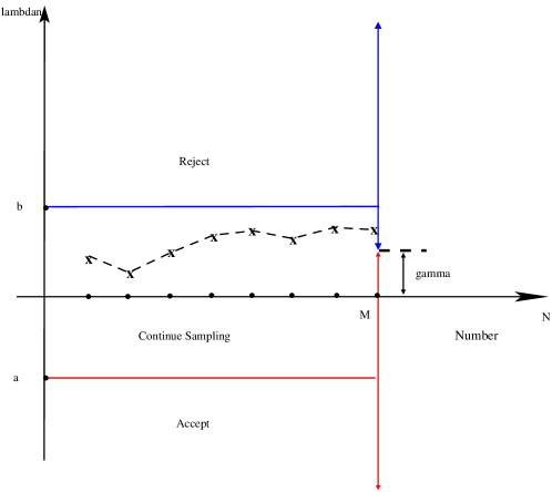
Figure 1: The test region of the SSCT.

In statistical term, the test procedure given in (10)–(12) is nothing but a truncated sequential test. As depicted in Fig. 1, the stopping boundaries of the test region consist of a horizonal line $b$ and a horizonal line $a$, which we simply call the upper- and lower-boundary respectively. Since each term in the cumulative sum $\Lambda_{N}$ is a shifted chi-square RV, we simply term the test procedure (10)-(12), the sequential shifted chi-square test. It is evident from (10)–(12) that the test statistic depends only on the amplitude squares of the received signal samples and the constant $\Delta$.

Let $r$ be a RV having the same PDF as $|r_{i}|^{2}-\Delta$, which is the $i$th incremental term in the test statistic (9). As we show below, we choose $\sigma_{w}^{2}<\Delta<\sigma_{w}^{2}(1+{\tt{SNR}}_{m})$ to ensure $E_{H_{0}}(r)<0<E_{H_{1}}(r)$ similar to the SPRT case. In the SSCT, we have $E_{H_{0}}(r)=\sigma_{w}^{2}-\Delta$ and $E_{H_{1}}(r)=\sigma_{w}^{2}(1+{\tt{SNR}}_{o})-\Delta$. Using ${\tt{SNR}}_{m}\leq{\tt{SNR}}_{o}$ and $\sigma_{w}^{2}<\Delta<\sigma_{w}^{2}(1+{\tt{SNR}}_{m})$, we always have $E_{H_{0}}(r)<0\leq{\tt{SNR}}_{o}-{\tt{SNR}}_{m}<E_{H_{1}}(r)$. Note that with this choice, the constant $\Delta$ depends on the minimum detection SNR instead of the exact operating SNR.

We normalize the test statistic $\Lambda_{N}$ by $\sigma_{w}^{2}/2$ and rewrite (9) as

$$\bar{\Lambda}_{N}=\sum_{i=1}^{N}(v_{i}-2\Delta/\sigma_{w}^{2})$$ (13)

where $\bar{\Lambda}_{N}:=2\Lambda_{N}/\sigma_{w}^{2}$ and $v_{i}:=2|r_{i}|^{2}/\sigma_{w}^{2}$. Let $\xi_{N}$ denote the sum of $v_{i}$ for $i=1,\ldots,N$, i.e., $\xi_{N}=\sum_{i=1}^{N}v_{i}$ and let $\bar{\Delta}$ denote $2\Delta/\sigma_{w}^{2}$. With this notation, we can rewrite $\bar{\Lambda}_{N}$ as

$$\bar{\Lambda}_{N}=\xi_{N}-N\bar{\Delta}.$$ (14)

For notional convenience, we define $\bar{\Lambda}_{0}$ and $\xi_{0}$ as zero. Let $a_{i}$ and $b_{i}$ be two parameters defined as follows: $a_{i}=0$ for $\aleph_{0}^{P}$, $a_{i}=\bar{a}+i\bar{\Delta}$ for $i\in\aleph_{P+1}^{\infty}$, and $b_{i}=\bar{b}+i\bar{\Delta}$ for $b\in\aleph_{0}^{\infty}$, where $\bar{a}:=2a/\sigma_{w}^{2}$, $\bar{b}:=2b/\sigma_{w}^{2}$, and $P$ denotes the largest integer not greater than $-a/\Delta$, i.e., $P:={\tt{floor}}(-a/\Delta)$. Using $\xi_{N}=\sum_{i=1}^{N}v_{i}$, we rewrite the test procedure (10)–(12) as

$$\mathtt{Reject}~{}H_{0}:~{} \mathtt{if}~{}\xi_{N}\geq b_{N}~{}\mathtt{and}~{}N\leq M-1,~{}\mathtt{or~{}if}~{}\xi_{M}\geq\bar{\gamma}_{M};$$ (15)

$$\mathtt{Accept}~{}H_{0}:~{} \mathtt{if}~{}\xi_{N}\leq a_{N}~{}\mathtt{and}~{}N\leq M-1,~{}\mathtt{or~{}if}~{}\xi_{M}<\bar{\gamma}_{M};~{}$$ (16)

$$\mathtt{Continue~{}Sensing}:~{} \mathtt{if}~{}\xi_{N}\in(a_{N},b_{N})~{}\mathtt{and}~{}N\leq M-1$$ (17)

where $\bar{\gamma}_{M}=\bar{\gamma}+M\bar{\Delta}$ with $\bar{\gamma}:=2\gamma/\sigma_{w}^{2}$. The corresponding test region is depicted in Fig. 2, where the stopping boundaries comprise two slant line segments. We adopt $\alpha_{\text{ssct}}$ and $\beta_{\text{ssct}}$ to denote the false-alarm and miss-detection probabilities of the SSCT, respectively.

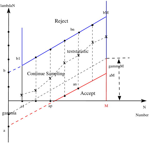
Figure 2: The test region of the transformed test procedure.

Since the proposed test procedure in (10)-(12) is not necessarily a SPRT, the Wald’s choice on thresholds, which yields a non-truncated SPRT satisfying specified false-alarm and miss-detection probabilities, is no longer applicable. Alternatively and conventionally, the thresholds $a$, $b$, $\gamma$, the parameter $\Delta$, and a truncated size $M$ are selected beforehand, either purposefully or randomly, and corresponding $\alpha_{\text{ssct}}$ and $\beta_{\text{ssct}}$ are then computed. If the resulted $\alpha_{\text{ssct}}$ and $\beta_{\text{ssct}}$ do not meet the requirement, the thresholds and truncated size are subsequently adjusted. This process continues until a desirable error probability performance is obtained. In the above process, the key step is to accurately and efficiently evaluate the false-alarm and miss-detection probabilities as well as the ASN for prescribed thresholds $a$, $b$, $\gamma$, the parameter $\Delta$, and a truncated size $M$, as will be addressed in the following section.

IV Evaluations of False-Alarm and Miss-Detection Probabilities

This section presents the exact false-alarm probability, and a numerical integration algorithm that obtains the miss-detection probability in a recursive manner [14]. We start by introducing some preparatory tools, including three mutually related integrals that will be frequently used in the evaluation of the false-alarm probability.

IV-A Preparatory Tools

The first integral is defined as

$$f^{(k)}_{\boldsymbol{\chi}_{k}}(\xi)=1,~{}k=0,~{}\text{and}~{}f^{(k)}_{\boldsymbol{\chi}_{k}}(\xi)=\int^{\xi}_{\chi_{k}}d\xi_{k}\int^{\xi_{k}}_{\chi_{k-1}}d\xi_{k-1}\cdots\int^{\xi_{2}}_{\chi_{1}}d\xi_{1},~{}k\geq 1$$ (18)

with $\boldsymbol{\chi}_{0}=\emptyset$ and $\boldsymbol{\chi}_{k}:=[\chi_{1},\ldots,\chi_{k-1},\chi_{k}]$ with $0\leq\chi_{1}\leq\ldots\leq\chi_{k}$. Note that superscript $k$ and subscript $\boldsymbol{\chi}_{k}$ are used to indicate that $f^{(k)}_{\boldsymbol{\chi}_{k}}(\xi)$ is a $k$-fold multiple integral with ordered lower limits specified by $\boldsymbol{\chi}_{k}$. Evidently, the integral $f_{\boldsymbol{\chi}_{k}}^{(k)}(\xi)$ is a polynomial in $\xi$ of degree $k$. The following lemma shows that the exact value of the integral $f^{(k)}_{\boldsymbol{\chi}_{k}}(\xi)$ can be obtained in a recursive manner (see Appendix A for the proof).

Lemma 1

The integral $f_{\boldsymbol{\chi}_{k}}^{(k)}(\xi)$ is given by

$$f_{\boldsymbol{\chi}_{k}}^{(k)}(\xi)=\sum_{i=0}^{k-1}\frac{f_{i}^{(k)}(\xi-\chi_{i+1})^{k-i}}{(k-i)!}+f_{k}^{(k)}$$ (19)

where the coefficients $f_{i}^{(k)},~{}i=0,\ldots,k$, for $k\geq 1$ can be computed by using the following recurrence relation

$$f_{i}^{(k)}=f_{i}^{(k-1)},~{}i\in\aleph_{0}^{k-1},~{}f_{k}^{(k)}=-\sum_{i=0}^{k-1}\frac{f_{i}^{(k-1)}}{(k-i)!}(\chi_{k}-\chi_{i+1})^{k-i}$$ (20)

and the initial conditions $f_{0}^{(0)}=1$. In particular, if $\chi_{1}=\chi_{2}=\ldots=\chi_{k}=\chi$, $f^{(k)}_{\boldsymbol{\chi}_{k}}$ is given by

$$f^{(k)}_{\boldsymbol{\chi}_{k}}=\frac{1}{k!}(\xi-\chi)^{k}.$$ (21)

Furthermore, the integral $f^{(k)}_{\boldsymbol{\chi}_{k}}(\xi)$ satisfies the following properties

1. Differential Property: $df^{(k)}_{\boldsymbol{\chi}_{k}}(\xi)/d\xi=f^{(k-1)}_{\boldsymbol{\chi}_{k-1}}(\xi)$ with $\boldsymbol{\chi}_{k-1}=[\chi_{1},\ldots,\chi_{k-1}]$ and $k\geq 2$;

2. Scaling Property: $f^{(k)}_{t\boldsymbol{\chi}_{k}}(t\xi)=t^{k}f_{\boldsymbol{\chi}_{k}}^{(k)}(\xi)$ for $t>0$;

3. Shift Property: $f^{(k)}_{\boldsymbol{\chi}_{k}-\delta{\mathbf{1}}_{k}}(\xi-\delta)=f^{(k)}_{\boldsymbol{\chi}_{k}}(\xi)$.

It is noteworthy to mention that scaling and shift properties are particularly useful in reducing round-off errors when evaluating $f^{(k)}_{\boldsymbol{\chi}_{k}}(\xi)$. We now introduce the second integral as

$$I^{(0)}:=1,~{}\text{and}~{}I^{(n)}:=\idotsint\limits_{\Omega^{(n)}}d\boldsymbol{\xi}_{n},~{}n\geq 1~{}$$ (22)

where $\boldsymbol{\xi}_{n}:=[\xi_{1},\xi_{2},\ldots,\xi_{n}]$ with $0\leq\xi_{1}\leq\xi_{2}\cdots\leq\xi_{n}$, and $\Omega^{(n)}=\{(\xi_{1},\xi_{2},\ldots,\xi_{n}):0\leq\xi_{1}\leq\cdots\leq\xi_{n};a_{i}<\xi_{i}<b_{i},i\in\aleph_{1}^{n}\}$. In particular, when $n=1$, $I^{(1)}=\int_{a_{1}}^{b_{1}}d\xi_{1}=b_{1}-a_{1}$. Let $c$ and $d$ denote two non-negative real numbers satisfying $0\leq c<d$, $a_{N-1}\leq c\leq b_{N}$ and $a_{N}\leq d$. Define the following vector

$$\boldsymbol{\psi}_{n,c}^{N}=\begin{cases}[\underset{Q}{\underbrace{b_{n+1},\ldots,b_{n+1}}},\underset{N-Q-n}{\underbrace{a_{Q+n+1},\ldots,a_{N-1},c}}],&n\in\aleph_{0}^{N-Q-2},\\ [\underset{N-n}{\underbrace{b_{n+1},\ldots,b_{n+1},c}}],&n\in\aleph_{N-Q-1}^{s-1},\\ b_{n+1}{\mathbf{1}}_{N-n},&n\in\aleph_{s}^{N-2},\end{cases}$$

where $s$ denotes the integer such that $b_{s}<c\leq b_{s+1}$, $Q$ denotes the integer such that $a_{Q}\leq b_{1}<a_{Q+1}$, and $N\geq 2$. Let ${\mbox{\boldmath$A$}}_{i}$ be an $(N-n)\times(N-n-i)$ matrix defined as ${\mbox{\boldmath$A$}}_{i}=[{\mbox{\boldmath$I$}}_{N-i-n}|{\mathbf{0}}_{(N-i-n)\times i}]^{T}$ with $i\in\aleph_{1}^{N-n}$. We further define the following vectors

$$\boldsymbol{\psi}^{N-i}_{n,c}=\boldsymbol{\psi}_{n,c}^{N}\cdot{\mbox{\boldmath$A$}}_{i},~{}i\in\aleph_{1}^{N-n},\quad{\mbox{\boldmath$a$}}^{n_{2}}_{n_{1}}=[a_{n_{1}+1},\ldots,a_{n_{2}}],~{}n_{2}\geq n_{1}\geq 0$$ (23)

where $\boldsymbol{\psi}^{N-i}_{n,c}$ is an $(N-i-n)\times 1$ vector and ${\mbox{\boldmath$a$}}_{n_{1}}^{n_{2}}$ is an $(n_{1}-n_{2})\times 1$ vector. In particular, $a_{n_{1}}^{n_{2}}$ is defined as $\emptyset$ when $n_{1}=n_{2}$.

We next show that the exact value of the integral $I^{(N)}$ in (22) can be obtained recursively as follows (see Appendix B for the proof).

Lemma 2

The exact value of the integral $I^{(N)}$ can be obtained by applying the following recurrence relation

$$I^{(N)}=\begin{cases}f^{(N)}_{{\mbox{\footnotesize\boldmath$a$}}^{N}_{0}}(b_{N})-\mathbb{I}_{\{N\geq 2\}}\displaystyle\sum_{n=0}^{N-2}\frac{(b_{N}-b_{n+1})^{N-n}}{(N-n)!}I^{(n)},&N\in\aleph_{1}^{Q}\\ f^{(N)}_{{\mbox{\footnotesize\boldmath$a$}}^{N}_{0}}(b_{N})-\displaystyle\sum_{n=0}^{N-2}f^{(N-n)}_{\boldsymbol{\psi}^{N}_{n,a_{N}}}(b_{N})I^{(n)},&N\in\aleph_{Q+1}^{\infty}\end{cases}$$ (24)

and the initial condition $I^{(0)}=1$.

We now introduce the third integral in the following

$$J^{(N)}_{c,d}(\theta): =\idotsint\limits_{\Upsilon_{c,d}^{(N)}}~{}e^{-\theta\xi_{N}}d\boldsymbol{\xi}_{N}$$ (25)

where $\theta>0$, $N\geq 1$, and $\Upsilon_{c,d}^{(N)}:=\{(\xi_{1},\ldots,\xi_{N}):0\leq\xi_{1}\leq\ldots\leq\xi_{N};a_{i}<\xi_{i}<b_{i},i\in\aleph^{N-1}_{1};c<\xi_{N}<d\}$. Recalling that $c$ is an arbitrary non-negative number satisfying $a_{N-1}\leq c\leq b_{N}$ and $d$ is an arbitrary number satisfying $0\leq c<d$ and $d\geq a_{N}$, we define the following function

$$g_{c,d}^{(n)}(\theta)=\begin{cases}\displaystyle I^{(n)}\Big{[}\theta^{n-N}e^{-\theta b_{n+1}}-\sum_{i=1}^{N-n}\theta^{-i}f^{(N-n-i)}_{b_{n+1}{\mathbf{1}}_{N-n-i}}(d)e^{-\theta d}\Big{]},&c\leq b_{1},~{}n\in\aleph_{0}^{N-2}\\ \displaystyle I^{(n)}\sum_{i=1}^{N-n}\theta^{-i}\Big{[}f^{(N-n-i)}_{{\boldsymbol{\psi}}_{n,c}^{N-i}}(c)e^{-\theta c}-f^{(N-n-i)}_{{\boldsymbol{\psi}}_{n,c}^{N-i}}(d)e^{-\theta d}\Big{]},&c>b_{1},~{}n\in\aleph_{0}^{s-1}\\ \displaystyle I^{(n)}\Big{[}\theta^{n-N}e^{-\theta b_{n+1}}-\sum_{i=1}^{N-n}\theta^{-i}f^{(N-n-i)}_{b_{n+1}{\mathbf{1}}_{N-n-i}}(d)e^{-\theta d}\Big{]},&c>b_{1},~{}n\in\aleph_{s}^{N-2}.\end{cases}$$

The following lemma shows the exact values of the integral $J^{(N)}_{c,d}(\theta)$ for two particular pairs of $(c,d)$ (see Appendix C for the proof).

Lemma 3

For any $\bar{\gamma}_{N}$ satisfying $a_{N}\leq\bar{\gamma}_{N}<b_{N}$, the exact values of the integrals $J^{(N)}_{\bar{\gamma}_{N},\infty}(\theta)$ and $J^{(N)}_{a_{N},b_{N}}(\theta)$ are given by

$$J^{(N)}_{\bar{\gamma}_{N},\infty}(\theta)= \sum_{i=1}^{N}\theta^{-i}f^{(N-i)}_{{\mbox{\footnotesize\boldmath$a$}}^{N-i}_{0}}(\bar{\gamma}_{N})e^{-\theta\bar{\gamma}_{N}}-\mathbb{I}_{\{N\geq 2\}}\sum_{n=0}^{N-2}g_{\bar{\gamma}_{N},\infty}^{(n)}(\theta)$$ (26)

$$J_{a_{N},b_{N}}^{(N)}(\theta)= \sum_{i=1}^{N}\theta^{-i}\Big{[}f^{(N-i)}_{{\mbox{\footnotesize\boldmath$a$}}^{N-i}_{0}}(a_{N})e^{-\theta a_{N}}-f^{(N-i)}_{{\mbox{\footnotesize\boldmath$a$}}^{N-i}_{0}}(b_{N})e^{-\theta b_{N}}\Big{]}-\mathbb{I}_{\{N\geq 2\}}\sum_{n=0}^{N-2}g^{(n)}_{a_{N},b_{N}}(\theta).$$ (27)

We next turn our attention to the evaluation of false-alarm and miss-detection probabilities.

IV-B False-Alarm Probability

Let $E_{N}$ denote the event that $\Lambda_{N}\geq b$ and $a<\Lambda_{n}<b$ for $n\in\aleph_{1}^{N-1}$ with $N\in\aleph_{1}^{M-1}$, and let $E_{M}$ denote the event that $\Lambda_{M}\geq\gamma$ and $a<\Lambda_{n}<b$ for $n\in\aleph_{1}^{M-1}$. Denote by $P_{H_{0}}(E_{N})$ the probability of the event $E_{N}$ under $H_{0}$. Recalling that the test procedure given in (10)-(12) is equivalent to that given in (15)-(17), we have

$$P_{H_{0}}(E_{N})=\begin{cases}P_{H_{0}}(a_{i}<\xi_{i}<b_{i},i\in\aleph_{1}^{N-1};\xi_{N}\geq b_{N}),&N\in\aleph_{1}^{M-1}\\ P_{H_{0}}(a_{i}<\xi_{i}<b_{i},i\in\aleph_{1}^{M-1};\xi_{M}\geq\bar{\gamma}_{M}),&N=M.\end{cases}$$ (28)

Clearly, the false-alarm probability $\alpha_{\text{ssct}}$ can be written $\alpha_{\text{ssct}}=\sum_{N=1}^{M}P_{H_{0}}(E_{N})$. In the following proposition, we present the exact false-alarm probability $\alpha_{\text{ssct}}$.

Proposition 1

The false-alarm probability, $\alpha_{\text{ssct}}$, is given by

$$\alpha_{\text{ssct}}=\sum_{N=1}^{M}P_{H_{0}}(E_{N})$$ (29)

where $P_{H_{0}}(E_{N})$ can be computed as

$$\!\!P_{H_{0}}(E_{N})\!=\!\begin{cases}\displaystyle\!p_{N}\frac{b_{1}b_{N}^{N-2}}{(N-1)!},&N\in\aleph_{1}^{P+1}\\ \!p_{N}\Big{[}f^{(N-1)}_{{\mbox{\footnotesize\boldmath$a$}}^{N-1}_{0}}(b_{N-1})\!-\!\mathbb{I}_{\{N\geq 3\}}\displaystyle{\sum_{n=0}^{N-3}}\frac{(b_{N-1}-b_{n+1})^{N-n-1}}{(N-n-1)!}2^{n}e^{\frac{b_{n+1}}{2}}P_{H_{0}}(E_{n+1})\Big{]},&N\in\aleph_{P+2}^{Q+1}\\ \!p_{N}\Big{[}f^{(N-1)}_{{\mbox{\footnotesize\boldmath$a$}}^{N-1}_{0}}(b_{N-1})\!-\!\displaystyle\sum_{n=0}^{N-3}f^{(N-1-n)}_{\boldsymbol{\psi}^{N-1}_{n,a_{N-1}}}(b_{N-1})2^{n}e^{\frac{b_{n+1}}{2}}P_{H_{0}}(E_{n+1})\Big{]},&N\in\aleph_{Q+2}^{M-1}\\ \!2^{-M}J_{\bar{\gamma}_{M},\infty}^{(M)}(1/2),&N=M\end{cases}$$

where $p_{N}:=2^{-(N-1)}e^{-b_{N}/2}$.

Proof:

To compute $P_{H_{0}}(E_{N})$, we need to determine the joint PDF of the RVs $(\xi_{1},\ldots,\xi_{N})$. Let $p_{{\mbox{\boldmath$v$}}|H_{0}}(v_{1},\ldots,v_{N}|H_{0})$ and $p_{\boldsymbol{\xi}|H_{0}}(\xi_{1},\ldots,\xi_{N}|H_{0})$ denote the joint PDFs of the RVs $(v_{1},\ldots,v_{N})$ and the RVs $(\xi_{1},\ldots,\xi_{N})$ under $H_{0}$, respectively. Recalling that $v_{i}$ is an exponential RV distributed according to (5), we can write the joint PDF of the RVs $(v_{1},\ldots,v_{N})$ as $p_{{\mbox{\boldmath$v$}}|H_{0}}(v_{1},\ldots,v_{N}|H_{0})=2^{-N}e^{-\sum_{i=1}^{N}v_{i}/2}$. Due to $\xi_{N}=\sum_{i=1}^{N}v_{i}$, we have $v_{1}=\xi_{1},v_{2}=\xi_{2}-\xi_{1},\ldots,v_{N}=\xi_{N}-\xi_{N-1}$, which yields

$$p_{\boldsymbol{\xi}|H_{0}}(\xi_{1},\xi_{2},\ldots,\xi_{N}|H_{0})=p_{{\mbox{\boldmath$v$}}|H_{0}}(\xi_{1},\xi_{2}-\xi_{1},\ldots,\xi_{N}-\xi_{N-1}|H_{0})=2^{-N}e^{-\xi_{N}/2},~{}$$ (30)

where $\xi_{0}:=0\leq\xi_{1}\leq\cdots\leq\xi_{N}$. According to (28) and the definition of $\Upsilon_{b_{N},\infty}^{(N)}$, we have

$$P_{H_{0}}(E_{N})=P_{H_{0}}\Big{(}(\xi_{1},\xi_{2},\ldots,\xi_{N})\in\Upsilon_{b_{N},\infty}^{(N)}\Big{)}=\idotsint\limits_{\Upsilon_{b_{N},\infty}^{(N)}}2^{-N}e^{-\xi_{N}/2}d\boldsymbol{\xi}_{N}.$$ (31)

Generally speaking, because each variable $\xi_{i}$ is lower-bounded by the maximum of $a_{i}$ and $\xi_{i-1}$, and is upper-bounded by the minimum of $b_{i}$ and $\xi_{i+1}$, a direct evaluation is highly complex due to numerous possibilities of upper- and lower-limits of $(\xi_{1},\xi_{2},\ldots,\xi_{N})$ [15].

Nevertheless, in the case of $N\in\aleph_{1}^{P+1}$, the parameters $a_{i}$ for $i\in\aleph_{1}^{N-1}$ are all zeros by the definition of the parameter $P$. This implies that $\xi_{i}$ is only lower-bounded by $\xi_{i-1}$ for $i\in\aleph_{1}^{N-1}$, and accordingly the upper-bound of $\xi_{i}$ can be readily identified as $b_{i}$ for $i\in\aleph_{1}^{N-1}$ [15]. Using [15, Eqs. (16) and (17)] and the fact that $\{b_{i}\}_{i=1}^{\infty}$ is an arithmetic sequence, we obtain $P_{H_{0}}(E_{N})$ as follows

$$P_{H_{0}}(E_{N})=\int_{\xi_{0}}^{b_{1}}d\xi_{1}\int_{\xi_{1}}^{b_{2}}d\xi_{2}\cdots\int_{\xi_{N-2}}^{b_{N-1}}d\xi_{N-1}\int_{b_{N}}^{\infty}2^{-N}e^{-\xi_{N}/2}d\xi_{N}=\frac{b_{1}b_{N}^{N-2}e^{-b_{N}/2}}{2^{N-1}(N-1)!}$$ (32)

with $N\in\aleph_{1}^{P+1}$.

We now consider the case of $N\in\aleph_{P+2}^{M-1}$. Since $\xi_{N}\in[b_{N},\infty)$ and $b_{N}>b_{N-1}$, the upper-limit of $\xi_{N-1}$ is actually $b_{N-1}$ irrespective of $\xi_{N}$. Hence, from (22), we can write (31) as

$$P_{H_{0}}(E_{N})=\int_{b_{N}}^{\infty}2^{-N}e^{-\xi_{N}/2}d\xi_{N}\cdot\idotsint\limits_{\Omega^{(N-1)}}d\boldsymbol{\xi}_{N-1}=2^{-(N-1)}e^{-b_{N}/2}I^{(N-1)}$$ (33)

with $N\in\aleph_{P+2}^{M-1}$. By applying (22), $P_{H_{0}}(E_{N})$ for $N\in\aleph_{P+2}^{Q+1}$ and $N\in\aleph_{Q+2}^{M-1}$ in (1) can be readily obtained.

We next compute $P(E_{M}|H_{0})$. Since $\bar{\gamma}_{M}\in(a_{M},b_{M})$, the upper-limit of $\xi_{M-1}$ depends on both $\xi_{M}$ and $b_{M-1}$. Thus, the integrals $\int d\xi_{M}$ and $\idotsint\limits d\boldsymbol{\xi}_{M-1}$ are not separable. It is clear from Lemma 3 that $P(E_{M}|H_{0})$ can be obtained from $J_{\bar{\gamma}_{M},\infty}^{(M)}(\theta)$ by setting $\theta=1/2$ and $N=M$ in (26). Hence, we have

$$P_{H_{0}}(E_{M})=P_{H_{0}}\big{(}(\xi_{1},\ldots,\xi_{M})\in\Upsilon_{\bar{\gamma}_{M},\infty}^{(M)}\big{)}=\idotsint\limits_{\Upsilon_{\bar{\gamma}_{M},\infty}^{(M)}}2^{-M}e^{-\xi_{M}/2}d\boldsymbol{\xi}_{M}=2^{-M}J_{\bar{\gamma}_{M},\infty}^{(M)}\big{(}1/2\big{)}.$$ (34)

Thanks to (32), (33), and (34), we can conclude the proof. ∎

Remark 1

The problem of evaluating (31) resembles the exact OC evaluation problem in truncated sequential life tests involving the exponential distribution [15]. Exact OC for truncated sequential life tests in the exponential case has been solved by Woodall and Kurkjian [15]. However, the Woodall-Kurkjian approach [15] is not applicable to evaluate the ASN [16]. More importantly, it cannot be used to evaluate (34) directly. In the preceding proof, we propose a new approach to derive the exact false-alarm probability $\alpha_{\text{ssct}}$. It is worth mentioning that with slight modifications, our approach is also applicable to evaluate the ASN for truncated sequential life tests in the exponential case.

IV-C Miss-Detection Probability

We now turn to the evaluation of the miss-detection probability, $\beta_{\text{ssct}}$. In order to evaluate $\beta_{\text{ssct}}$, we need to obtain $p_{H_{1}}(v_{i})$. Since acquiring perfect knowledge on instantaneous $\lambda_{i}$ or the exact distribution of $\lambda_{i}$ may not be feasible in practice, evaluating $p_{H_{1}}(v_{i})$ is typically difficult except for the case where the primary signals are constant-modulus, i.e., $|s_{i}|^{2}=\sigma_{s}^{2}$. We next reason that at a relatively low detection SNR level, the miss-detection probability obtained by using constant-modulus primary signals can be used to well approximate the actual $\beta_{\text{ssct}}$. Our arguments are primarily based on the following two properties of the SSCT.

The first property shows that as $N$ approaches infinity, the distribution of the test statistic $\xi_{N}$ in the SSCT converges to a normal distribution that is independent of a specific choice of $\lambda_{1},\lambda_{2},\ldots,\lambda_{N}$.

Property 1

The statistical distribution of $\xi_{N}$ converges to a normal distribution given by

$$\xi_{N}\sim\begin{cases}\mathcal{N}(2N,4N),&\text{under}~{}H_{0},\\ \mathcal{N}\big{(}2N(1+{\tt{SNR}}_{m}),4N(1+2{\tt{SNR}}_{m})\big{)},&\text{under}~{}H_{1},\end{cases}$$

as $N$ approaches infinity.

The property can be readily proved by using the CLT [17]. However, unlike energy detection, this property alone is not sufficient to explain that the constant-modulus assumption is valid in approximating $\beta_{\text{ssct}}$. This is because each $\xi_{N}$ for $N=1,\ldots,M$ including small values of $N$, may potentially affect the value of $\beta_{\text{ssct}}$. To complete our argument, we first present the following definitions. Let $\tilde{\xi}_{i}$ denote the test statistic using the constant-modulus assumption, i.e., $|s_{i}|^{2}=\sigma_{s}^{2}$. Define $\varrho_{N}:=b_{N}$ for $N\in\aleph_{1}^{M-1}$ and $\varrho_{M}:=\bar{\gamma}_{M}$ for $N=M$. Let $F_{N}$ and $\tilde{F}_{N}$ denote the events that $\xi_{N}\geq\varrho_{N}$, and $a_{i}<\xi_{i}<b_{i}$ for $i\in\aleph_{1}^{M}$, and $\tilde{\xi}_{N}\geq\varrho_{N}$ and $a_{i}<\tilde{\xi}_{i}<b_{i}$ for $i\in\aleph_{1}^{M}$, respectively. Let $P_{H_{1}}(F_{N})$ and $P_{H_{1}}(\tilde{F}_{N})$ denote the probabilities of the events $F_{N}$ and $\tilde{F}_{N}$ under $H_{1}$. Let $\tilde{\beta}_{\text{ssct}}$ denote the miss-detection probability obtained by assuming constant-modulus signals with average symbol energy $\sigma_{s}^{2}$, i.e., $|s_{i}|^{2}=\sigma_{s}^{2}$. As clear from their definitions, we have $\beta_{\text{ssct}}=\sum_{N=1}^{M}P_{H_{1}}(F_{N})$ and $\tilde{\beta}_{\text{ssct}}=\sum_{N=1}^{M}P_{H_{1}}(\tilde{F}_{N})$.

Let $\mathcal{A}_{N}^{l_{N}}$ denote the event that $a_{i}<\xi_{i}<b_{i},~{}i\in\aleph_{1}^{l_{N}}$ for some integer $l_{N}\in\aleph_{1}^{N}$, and let $\tilde{\mathcal{A}}_{N}^{l_{N}}$ denote its counterpart for the constant-modulus case. Let $\mathcal{B}_{N}^{l_{N}}$ denote the event that $\xi_{N}\geq\varrho_{N}$ and $a_{i}<\xi_{i}<b_{i},~{}i\in\aleph_{l_{N}+1}^{N}$ and let $\tilde{\mathcal{B}}_{N}^{l_{N}}$ denote its counterpart in the constant-modulus case. We now present the second property of the SSCT (see Appendix D for the proof).

Property 2

Let $\epsilon$ an arbitrary positive number. If for each $N$, there exists a positive integer $l_{N}\in\aleph_{1}^{N}$ such that $P_{H_{1}}(\mathcal{A}_{N}^{l_{N}})\geq 1-\epsilon/(3M)$, $P_{H_{1}}(\tilde{\mathcal{A}}_{N}^{l_{N}})\geq 1-\epsilon/(3M)$, and $|P_{H_{1}}(\mathcal{B}_{N}^{l_{N}})-P_{H_{1}}(\tilde{\mathcal{B}}_{N}^{l_{N}})|<\epsilon/(3M)$, then

$$|\beta_{\text{ssct}}-\tilde{\beta}_{\text{ssct}}|\leq\epsilon$$

where $l_{N}$ depends on the values of $N$ and $\epsilon$.

Relying on these two properties, we sketch our arguments as follows. To achieve high detection accuracy at a low SNR level, the ASN and $M$ are typically quite large. When the sample index $N$ is relatively small, it is highly likely that the test statistics $\xi_{N}$ and $\tilde{\xi}_{N}$ do not cross either of two boundaries. In such a situation, there exists some integer $l_{N}$ such that $P_{H_{1}}(\mathcal{A}_{N}^{l_{N}})$ and $P_{H_{1}}(\tilde{\mathcal{A}}_{N}^{l_{N}})$ are fairly close to $1$ whereas $P_{H_{1}}(\mathcal{B}_{N}^{l_{N}})$ and $P_{H_{1}}(\tilde{\mathcal{B}}_{N}^{l_{N}})$ are fairly close to $0$. Hence, the conditions in Property 2 can be easily satisfied. On the other hand, when $N$ is relatively large, one can find a sufficiently large $l_{N}$ such that $P_{H_{1}}(\mathcal{A}_{N}^{l_{N}})$ and $P_{H_{1}}(\tilde{\mathcal{A}}_{N}^{l_{N}})$ are fairly close to one while $|P_{H_{1}}(\mathcal{B}_{N}^{l_{N}})-P_{H_{1}}(\tilde{\mathcal{B}}_{N}^{l_{N}})|$ are sufficiently small due to Property 1 guaranteed by the CLT. Collectively, at a low detection SNR level, $\tilde{\beta}_{\text{ssct}}$ evaluated under the constant-modulus assumption is a close approximation of $\beta_{\text{ssct}}$. Therefore, we will focus on the case in which all $\lambda_{i}$’s are equal to a constant $\lambda:=2|h|^{2}\sigma_{s}^{2}/\sigma_{w}^{2}=2{\tt{SNR}}_{m}$.

Recall that under $H_{1}$, $v_{i}$ is a non-central chi-square RV, whose PDF involves the zeroth-order modified Bessel function of the first kind as given in (6). This makes it infeasible to evaluate $\tilde{\beta}_{\text{ssct}}$ by applying the computational approach used in the false-alarm probability case. To obtain $\tilde{\beta}_{\text{ssct}}$, we resort to a numerical integration algorithm proposed in [14].

Defining $u_{i}=v_{i}-\bar{\Delta}$, we rewrite $\bar{\Lambda}_{N}$ in (13) as $\bar{\Lambda}_{N}=\sum_{i=1}^{N}u_{i}$. Clearly, we can write the PDF of $u_{i}$ under $H_{1}$ as

$$p_{H_{1}}(u_{i})=\frac{1}{2}e^{-(u_{i}+\bar{\Delta}+\lambda)}I_{0}\Big{(}\sqrt{\lambda(u_{i}+\bar{\Delta})}\Big{)},u_{i}>-\bar{\Delta}.$$ (35)

Recall that $M$ is the maximum number of samples to observe. Denote $\bar{\Lambda}_{M-k}$ by $t_{k}$. Let $G_{k}(t_{k})$ denote the conditional miss-detection probability of the SSCT conditioning on that the first $(M-k)$ samples have been observed, the present value $t_{k}=\bar{\Lambda}_{M-k}$, and the test statistic has not crossed either boundary in the previous $(M-k-1)$ samples. If $\bar{a}<t_{k}<\bar{b}$, an additional sample (the $(M-k+1)$th sample) is needed. Let $u$ be the next observed value of $u_{i}$. The conditional probability $G_{k}(t_{k}|u)$ can be written as

$$G_{k}(t_{k}|u)=\begin{cases}0&\textrm{if}~{}u>\bar{b}-t_{k}\\ 1&\textrm{if}~{}u<\bar{a}-t_{k}\\ G_{k-1}(t_{k}+u)&\textrm{if}~{}\bar{a}-t_{k}\leq u\leq\bar{b}-t_{k}.\end{cases}$$ (36)

Using (36), we can compute $G_{k}(t_{k})$ as

$$G_{k}(t_{k})=\int_{-\infty}^{\bar{a}-t_{k}}p_{H_{1}}(u)du+\int_{\bar{a}-t_{k}}^{\bar{b}-t_{k}}G_{k-1}(t_{k}+u)p_{H_{1}}(u)du$$ (37)

for $k=1,\cdots,M$ with the following initial condition:

$$G_{0}(t_{0})=\begin{cases}0,&\textrm{ if }t_{0}\geq\bar{\gamma}\cr 1,&\textrm{ otherwise.}\end{cases}$$ (38)

Employing the above backward recursion process, we can obtain $G_{M}(0)$, which is equal to the miss-detection probability, $\tilde{\beta}_{\text{ssct}}$.

V Evaluation of the Average Sample Number

Roughly speaking, the false-alarm and miss-detection probabilities, and the ASN are three principal performance benchmarks for the sequential sensing scheme. In the preceding section, we have only concerned ourselves with the error probability performance while in this section, we show how to evaluate the ASN.

Let $N_{s}$ denote the number of samples required to yield a decision. Clearly, $N_{s}$ is a RV in the SSCT, and its mean value is the ASN, which can be written as

$$E(N_{s})=E_{H_{0}}(N_{s})P_{H_{0}}(H_{0})+E_{H_{1}}(N_{s})P_{H_{1}}(H_{1})$$ (39)

where $E_{H_{i}}(N_{s})$ denotes the ASN conditional on $H_{i}$, and $P_{H_{i}}(H_{i})$ denotes a priori probability of hypothesis $H_{i}$, for $i=0,1$.

According to (10)–(12), we have $1\leq N_{s}\leq M$. Hence, we can express $E_{H_{i}}(N_{s})$ as

$$E_{H_{i}}(N_{s})=\sum_{N=1}^{M}NP_{H_{i}}(N_{s}=N),~{}i=0,1$$ (40)

where $P_{H_{i}}(N_{s}=N)$ is the conditional probability that the detector makes a decision at the $N$th sample under $H_{i}$. We now need to determine $P_{H_{i}}(N_{s}=N)$. Let ${\mathcal{C}}_{N}$ denote the event that the test statistics $(\xi_{1},\xi_{2},\ldots,\xi_{N})$ do not cross either the upper or lower boundary before or at the $N$th sample, i.e., ${\mathcal{C}}_{N}=\{(\xi_{1},\xi_{2},\ldots,\xi_{N})\in\Upsilon_{a_{N},b_{N}}^{(N)}\}$ for $N\in\aleph_{1}^{M}$. For notional convenience, let us define ${\mathcal{C}}_{0}$ as a universe set. Hence, we have $P({\mathcal{C}}_{0})=1$. It implies from (15)-(17) that $P_{H_{i}}(N_{s}=N),~{}i=0,1$ can be obtained as

$$P_{H_{i}}(N_{s}=N) \overset{(a)}{=}P_{H_{i}}\big{(}{\mathcal{C}}_{N-1}\big{)}-P_{H_{i}}\big{(}{\mathcal{C}}_{N}\big{)},~{}N\in\aleph_{1}^{M-1}$$ (41)

$$P_{H_{i}}(N_{s}=M) \overset{(b)}{=}P_{H_{i}}\big{(}{\mathcal{C}}_{M-1}\big{)},\quad\quad\quad\quad\quad N=M$$ (42)

where the two terms on the right-hand side (RHS) of the equality $(a)$ are the probabilities of the events that under $H_{i}$, the test statistic does not cross either of two boundaries before or at the $(N-1)$th sample and the $N$th sample for $N\in\aleph_{1}^{M-1}$, respectively, and the term on the RHS of the equality $(b)$ denotes the probability of the event that under $H_{i}$, the test statistic does not cross either boundary before or at the $(M-1)$th sample.

Substituting (41) and (42) in (40), we can rewrite (40) as

$$E_{H_{i}}(N_{s})=\sum_{N=1}^{M-1}N\Big{(}P_{H_{i}}\big{(}{\mathcal{C}}_{N-1}\big{)}-P_{H_{i}}\big{(}{\mathcal{C}}_{N}\big{)}\Big{)}+MP_{H_{i}}\big{(}{\mathcal{C}}_{M-1}\big{)}=1+\sum_{N=1}^{M-1}P_{H_{i}}\Big{(}{\mathcal{C}}_{N}\Big{)}.$$ (43)

According to Lemma 3, (30), (41), and (42), we have

$$P_{H_{0}}\big{(}{\mathcal{C}}_{N}\big{)}=2^{-N}J^{(N)}_{a_{N},b_{N}}(1/2),~{}N\in\aleph_{1}^{M-1}.$$ (44)

Hence, from (43), we have

$$E_{H_{0}}(N_{s})=1+\sum_{N=1}^{M-1}2^{-N}J^{(N)}_{a_{N},b_{N}}(1/2).$$ (45)

We next need to evaluate $P_{H_{1}}({\mathcal{C}}_{N})$. Instead of evaluating $P_{H_{1}}({\mathcal{C}}_{N})$ directly, we compute $P_{H_{1}}({\mathcal{C}}^{c}_{N})$ by performing a procedure similar to the one in calculating the miss-detection probability. Note that ${\mathcal{C}}_{N}^{c}$ denotes the event that under $H_{1}$, the test procedure given in (15)-(17) terminates before or at the $N$th sample, i.e., the test statistic crosses either the upper or lower boundary before or at the $N$th sample. According to (38), $G_{k}(t_{k})$ also depends on $\bar{\gamma}$. With a slight abuse of notation, we rewrite $G_{k}(t_{k})$ as $G_{k}(t_{k},\bar{\gamma})$. Let $V_{N}$ denote the event that the test statistic crosses the lower boundary before or at the $N$th sample under $H_{1}$, and $U_{N}$ denote the event that the test statistic does not cross the upper-boundary before or at the $N$th sample under $H_{1}$. It is clear to see $P_{H_{1}}(V_{N})=G_{N}(0,\bar{a})$ and $P_{H_{1}}(U_{N})=G_{N}(0,\bar{b})$. Obviously, $P_{H_{1}}(\mathcal{C}_{N}^{c})$ can be written as

$$P_{H_{1}}\big{(}{\mathcal{C}}_{N}^{c}\big{)}=P_{H_{1}}(V_{N})+(1-P_{H_{1}}(U_{N}))=G_{N}(0,\bar{a})+1-G_{N}(0,\bar{b})$$ (46)

where $G_{N}(t,\bar{a})$ and $G_{N}(t,\bar{b})$ can be obtained by applying (37) recursively. Hence, we have $P_{H_{1}}({\mathcal{C}}_{N})=G_{N}(0,\bar{b})-G_{N}(0,\bar{a})$. According to (43), we have

$$E_{H_{1}}(N_{s})=1+\sum_{N=1}^{M-1}(G_{N}(0,\bar{b})-G_{N}(0,\bar{a})).$$ (47)

In the following proposition, we present the ASN of the SSCT.

Proposition 2

The ASN of the SSCT can be obtained as

$$E(N_{s})= ~{}P_{H_{0}}(H_{0})\Big{(}1+\sum_{N=1}^{M-1}2^{-N}J^{(N)}_{a_{N},b_{N}}(1/2)\Big{)}+P_{H_{1}}(H_{1})\Big{(}1+\sum_{N=1}^{M-1}(G_{N}(0,\bar{b})-G_{N}(0,\bar{a}))\Big{)}.$$ (48)

Proof:

The proof follows immediately from (39), (45), and (47). ∎

VI Simulations

In this section, we provide several examples to illustrate the effectiveness of the SSCT. In all simulation examples, we select $\bar{\Delta}$ to be $2+{\tt{SNR}}_{m}$, which ensures $E_{H_{0}}(\Lambda_{N})=-E_{H_{1}}(\Lambda_{N})$. In the first three test examples, the truncated sample size $M$ is selected to be the minimum sample number $M_{\text{ed}}^{\min}$ required by energy detection to achieve specified false-alarm and miss-detection probabilities, and $\bar{a}$ is always chosen to be $-\bar{b}$. All the test examples assume that $|h|$ is equal to one, and adopt constant-modulus quadrature phase shift-keying (QPSK) signals except for Test Example 2, in which the modulation formats of the primary signals are explicitly stated. Following the conventional terminology in sequential detection, we define the efficiency of the SSCT as $\eta:=1-\text{ASN}/M_{\text{ed}}^{\min}$.

Test Example 1 (The SSCT Versus Energy Detection): Table I compares the SSCT with energy detection in terms of false-alarm and miss-detection probabilities and the ASN for different ${\tt{SNR}}_{m}$. The truncated sizes corresponding to ${\tt{SNR}}_{m}=0$, $-5$, $-10$, and $-15$ dB, are selected to be the minimum sample sizes required by energy detection to achieve target $(\bar{\alpha}_{\text{ssct}},\bar{\beta}_{\text{ssct}})=(0.01,0.01)$, $(0.05,0.05)$, $(0.1,0.1)$, and $(0.15,0.15)$, respectively. The parameters $\bar{b},~{}\bar{\Delta}$ and $\bar{\gamma}$ are given in the table. It is shown in Table I that compared with energy detection, the SSCT can achieve about $29\%\sim 35\%$ savings in the average sensing time while maintaining a comparable detection performance. It can be also observed from the table that, as indicated by using an abbreviation, Numerical, in the parenthesis, the false-alarm probabilities computed from the exact result (1) and the miss-detection probabilities obtained by the numerical integration algorithm match well with those obtained by Monte Carlo simulations.

Test Example 2 (Detection Performance Without Knowing the Modulation Format of the Primary Signals): In this example, the primary signals are modulated by using a square 64-quadrature amplitude modulation (QAM) with $\sigma_{s}^{2}=10^{{{\tt{SNR}}_{m}}/10}\sigma_{w}^{2}$. Table II compares with the miss-detection probabilities and the ASN between the SSCT and energy detection for ${\tt{SNR}}_{m}=0$, $-5$, $-10$, and $-15$ dB. The parameters $\bar{a}$, $\bar{b}$, $\bar{\gamma}$, $\bar{\Delta}$, and $M$ in the SSCT, are determined by using constant-modulus QPSK signals with the same average symbol energy $\sigma_{s}^{2}=10^{{\text{SNR}_{m}}/10}\sigma_{w}^{2}$, and these design parameters are used in the SSCT to detect the 64-QAM primary signals. That is, the SSCT does not have the knowledge of the modulation format of the primary signals. When evaluating the miss-detection probability and the ASN of the SSCT in the 64-QAM case, we use equiprobable prior distributions of $s_{i}$ to obtain $p_{H_{1}}(u_{i})$. As can be seen from the table, the miss-detection probabilities obtained in the 64-QAM case are fairly close to the ones obtained in the QPSK case except for the case of ${\tt{SNR}}_{m}=0$ dB, where $M=40$. This is because $M$ is not large enough to neglect errors caused by using the CLT approximation. However, energy detection and the SSCT suffer from a similar amount of approximation error when evaluating the miss-detection probability.

Test Example 3 (Mismatch between ${\tt{SNR}}_{o}$ and ${\tt{SNR}}_{m}$): Table III lists the false-alarm and miss-detection probabilities and ASN when ${\tt{SNR}}_{o}=-12$, $-13$, $-14$ dB, and ${\tt{SNR}}_{m}=-15$ dB. The parameters for the SSCT and energy detection are determined to ensure that a target pair $(\alpha_{\text{ssct}},\beta_{\text{ssct}})$ satisfies $(0.15,0.15)$ at ${\tt{SNR}}_{m}=-15$ dB. It can be seen from the table that, as ${\tt{SNR}}_{o}$ increases, the miss-detection probability decreases while the false-alarm probability remains unchanged. All obtained $(\alpha_{\text{ssct}},\beta_{\text{ssct}})$ pairs satisfy the target false-alarm and miss-detection probability requirement. Interestingly, the efficiency of the SSCT increases to $46\%$ from $29\%$ even though the miss-detection probabilities of the SSCT are larger than those in energy detection. It implies from this example that the SSCT offers more flexibility in striking the tradeoff between sensing time and detection performance than energy detection.

Test Example 4 (Impacts of Truncated Size $M$ on the Efficiency of the SSCT): Let $T_{p}$ denote the probability of the event that the SSCT ends at the $M$th sample (truncated at the $M$th sample). Table IV lists $T_{p}$, the ASN, and the efficiency of the SSCT for various selected combinations of $M$, $\bar{a}$, $\bar{b}$, and $\bar{\gamma}$ at ${\tt{SNR}}_{m}=-5$ dB to achieve target $(\bar{\alpha}_{\text{ssct}},\bar{\beta}_{\text{ssct}})=(0.055,0.046)$. The results shown in the table are obtained by using Monte Carlo simulation. To achieve roughly the same false-alarm and miss-detection probabilities, the sample size for energy detection is chosen to be $140$. As can be seen from this table, the efficiency of the SSCT increases as the truncated size $M$ increases but the pace of the improvement is diminishing. Table IV also lists the efficiency of the non-truncated SPRT based sensing scheme presented in Section II-B2. It is clear from the table that as the truncated size $M$ increases, the efficiency of the SSCT comes fairly close to the one achieved by the non-truncated SPRT based sensing scheme.

VII Conclusion

In cognitive radio networks, stringent requirements on the secondary and opportunistic access to licensed spectrum, necessitate the need to develop a spectrum sensing scheme that is able to quickly detect weak primary signals with high accuracy in a non-coherent fashion. Motivated by this, we have proposed a sequential sensing scheme that possesses several desirable features suitable for cognitive radio networks. To efficiently and accurately obtain major performance benchmarks of our sensing scheme, we have derived an exact result for the false-alarm probability and have applied a numerical integration algorithm to compute the miss-detection probability and the ASN.

There are several potential extensions of this work that deserve further exploration. First, our approach to determining design parameters such as thresholds and the truncated size follows the original Wald’s approach in the sense that the cost of observations as well as the cost of the false-alarm and miss-detection events have not been considered. A Bayesian formulation of the SSCT can be an interesting extension. Second, this work assumes perfect knowledge on noise power at the SU, which perhaps is difficult to acquire in practice. The effect of noise power uncertainty on the SSCT is worth investigating. Third, another extension of this work is to study sensing-throughput tradeoffs for the SSCT.

Appendix A Proof of Lemma 1

We prove the lemma by induction. It is obvious from (18) that (19) holds for $k=1$. Now suppose that (19) and (20) hold for the case of $k-1$. By definition and the induction assumption for $k-1$, we have

$$f_{\boldsymbol{\chi}_{k}}^{(k)}(\xi) =\int_{\chi_{k}}^{\xi}\left(\sum_{i=0}^{k-2}\frac{f_{i}^{(k-1)}}{(k-1-i)!}(\xi_{k-1}-\chi_{i+1})^{k-1-i}+f_{k-1}^{(k-1)}\right)d\xi_{k-1}$$

$$=\sum_{i=0}^{k-2}\frac{f_{i}^{(k-1)}}{(k-i)!}(\xi_{k-1}-\chi_{i+1})^{k-i}\Big{|}_{\chi_{k}}^{\xi}+f_{k-1}^{(k-1)}\cdot(\xi-\chi_{k})$$

$$=\sum_{i=0}^{k-1}\frac{f_{i}^{(k-1)}}{(k-i)!}(\xi-\chi_{i+1})^{k-i}-\sum_{i=0}^{k-2}\frac{f_{i}^{(k-1)}}{(k-i)!}(\chi_{k}-\chi_{i+1})^{k-i}.$$ (49)

Clearly, comparing (19) with (49), we can readily conclude the recurrence relation given in (20). In particular, when $\chi_{1}=\chi_{2}=\ldots=\chi_{k}$, all coefficients $f_{i}^{(k)}$ except $f_{0}^{(k)}$ are zeros and hence (21) follows immediately.

Since the differential property can be proved in a straightforward manner, we omit the proof. We next prove the scaling property by induction. When $k=1$, we have

$$f_{t{\boldsymbol{\chi}_{1}}}^{(1)}(t\xi)=\int_{t\chi_{1}}^{t\xi}d\xi_{1}=t(\xi-\chi_{1})=tf_{\boldsymbol{\chi}_{1}}^{(1)}(\xi).$$

Hence, the scaling property holds for $k=1$. We now suppose that the property holds for $k=n-1$. Applying the induction assumption and a substitution $t\xi_{n}=u$, we can rewrite the integral $f_{\boldsymbol{\chi}_{n}}^{(n)}(\xi)$ as

$$f_{\boldsymbol{\chi}_{n}}^{(n)}(\xi)=\int_{\chi_{n}}^{\xi}f_{\boldsymbol{\chi}_{n-1}}^{(n-1)}(\xi_{n})d\xi_{n}=\int_{\chi_{n}}^{\xi}t^{-(n-1)}f_{t\boldsymbol{\chi}_{n-1}}^{(n-1)}(t\xi_{n})d\xi_{n}=t^{-n}\int_{t\chi_{n}}^{t\xi}f_{t\boldsymbol{\chi}_{n-1}}^{(n-1)}(u)du=t^{-n}f_{t\boldsymbol{\chi}_{n}}^{(n)}(t\xi).$$

Hence, the scaling property holds for $k=n$. This concludes the proof. The shift property can be proved in a similar manner and thus the proof is omitted. $\blacksquare$

Appendix B Proof of Lemma 2

Recall that $\xi_{N}$ is a sum of $v_{i}$, i.e., $\xi_{N}=\sum_{i=1}^{N}v_{i}$ with $v_{i}=2|r_{i}|^{2}/\sigma_{w}^{2}$. Hence, $(\xi_{1},\xi_{2},\ldots,\xi_{N})$ is a non-decreasing sequence, i.e., $\xi_{0}\leq\xi_{1}\leq\xi_{2}\leq\cdots\leq\xi_{N}$. Fig. 3(a) plots the parameter $\xi_{N}$ versus the sample index $N$. It is clear from its definition that the region $\Omega^{(N)}$ contains all possible sequences $(\xi_{1},\xi_{2},\ldots,\xi_{N})$ (simply called paths hereafter) satisfying $\xi_{0}\leq\xi_{1}\leq\xi_{2}\leq\ldots\leq\xi_{N}$ and $0\leq a_{i}<\xi_{i}<b_{i}$. Hence, the $i$th component of each path $(\xi_{1},\xi_{2},\ldots,\xi_{N})$ in $\Omega^{(N)}$ is lower-bounded by the maximum of $\xi_{i-1}$ and $a_{i}$, and is upper-bounded by the minimum of $\xi_{i+1}$ and $b_{i}$. The direct computation of $I^{(N)}$ is highly complex [15] due to numerous possibilities for lower- and upper-limits in the integral $I^{(N)}$. Considering the fact that the integral $I^{(N)}$ can be readily computed if either the lower- or upper-limit is a constant, we express $\Omega^{(N)}$ into an equivalent set, over which the integration can be readily computed in a recursive fashion, thereby obviating the need to exhaustively enumerate these possibilities.

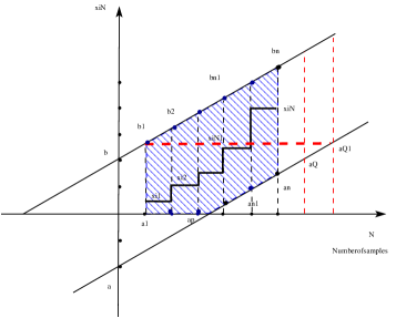
(a) Possible Paths from $\Omega^{(N)}~{}(N\leq Q)$.

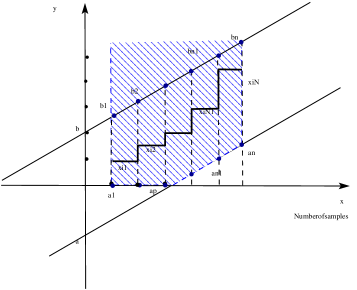
(b) Possible Paths from $\Pi_{{\mbox{\boldmath$a$}}^{N}_{0}}^{(N)}$.

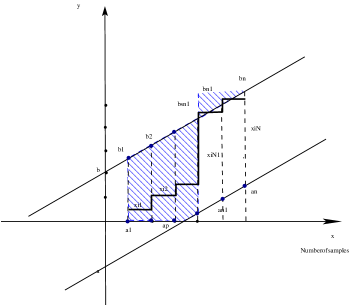
(c) Possible Paths from $\Xi_{n}^{(N)}$.

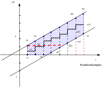
(d) Possible Paths from $\Omega^{(N)}~{}(N>Q)$.

Figure 3: An illustration for Proof of Lemma 2.

Let $\phi_{i},~{}i\in\aleph_{1}^{N}$, denote a sequence of real numbers with $0\leq\phi_{1}\leq\phi_{2}\leq\ldots\leq\phi_{N}$. Let us first define the following set,

$$\Pi^{(N-n)}_{\boldsymbol{\phi}_{n}^{N}}=\{ (\xi_{n+1},\xi_{n+2},\ldots,\xi_{N}):$$

$$0\leq\xi_{n+1}\leq\xi_{n+2}\ldots\leq\xi_{N};\phi_{i}<\xi_{i}\leq\xi_{i+1},i\in\aleph_{n+1}^{N-1};\phi_{N}<\xi_{N}<b_{N}\}$$ (50)

where $\boldsymbol{\phi}_{n}^{N}:=[\phi_{n+1},\ldots,\phi_{N}]$ is an $(N-n)$-dimensional real vector with the $i$th entry of the vector $\boldsymbol{\phi}_{n}^{N}$ being the lower bound of $\xi_{n+i}$ for $i\in\aleph_{1}^{N-n}$. We next define the following non-overlapping subsets of $\Pi_{{\mbox{\footnotesize\boldmath$a$}}_{0}^{N}}^{(N)}$,

$$\Xi^{(N)}_{n}:=\{ (\xi_{1},\ldots,\xi_{N}):(\xi_{1},\ldots,\xi_{N})\in\Pi_{{\mbox{\footnotesize\boldmath$a$}}_{0}^{N}}^{(N)},a_{i}<\xi_{i}<b_{i},i\in\aleph_{1}^{n};b_{n+1}\leq\xi_{n+1}\leq\xi_{n+2}\}$$ (51)

where $n\in\aleph_{0}^{N-2}$.

As can be seen from Figs. 3(b) and 3(c), $\Pi^{(N)}_{{\mbox{\footnotesize\boldmath$a$}}_{0}^{N}}$ contains all possible paths, $(\xi_{1},\xi_{2},\ldots,\xi_{N})$, which are lower-bounded by $(a_{1},a_{2},\ldots,a_{N})$ and upper-bounded by $(\xi_{2},\xi_{3},\ldots,\xi_{N},b_{N})$, whereas $\Xi^{(N)}_{n}$ for $n\in\aleph_{0}^{N-2}$ contains all possible paths $(\xi_{1},\xi_{2},\ldots,\xi_{N})$ having the property that the first $n$ variables lie in the set $\Omega^{(n)}$, i.e., $(\xi_{1},\ldots,\xi_{n})\in\Omega^{(n)}$, and the $(n+1)$th variable $\xi_{n+1}$ excesses the upper slant line, i.e., $\xi_{n+1}\geq b_{n+1}$. Again, it is clear from its definition that the set $\Omega^{(N)}$ is equal to the difference between the set $\Pi^{(N)}_{{\mbox{\footnotesize\boldmath$a$}}_{0}^{N}}$ and the union of $\Xi^{(N)}_{n}$ for $n\in\aleph_{0}^{N-2}$, i.e., $\Omega^{(N)}=\Pi^{(N)}_{{\mbox{\footnotesize\boldmath$a$}}_{0}^{N}}\cap\big{(}\cup_{n=0}^{N-2}\Xi^{(N)}_{n}\big{)}^{c}$. Thus, it follows from (22) that

$$I^{(N)}=\idotsint\limits_{\Pi^{(N)}_{{\mbox{\footnotesize\boldmath$a$}}_{0}^{N}}}d\boldsymbol{\xi}_{N}-\sum_{n=0}^{N-2}\idotsint\limits_{\Xi^{(N)}_{n}}d\boldsymbol{\xi}_{N}.$$ (52)

We now evaluate two terms on the right-hand side (RHS) of (52). It is clear from (18) and (B) that the first term on the RHS of (52) is nothing but $f_{{\mbox{\footnotesize\boldmath$a$}}_{0}^{N}}^{(N)}(b_{N})$. We next take a close look at the second term. The evaluation of the second term is categorized into the following two cases:

• Case 1: $N\leq Q$: In this case, we have $b_{n+1}>b_{1}\geq a_{n}$ for any $n\in\{1,\ldots,N\}$. It implies from (51) that we can express $\Xi^{(N)}_{n}$ as $\Xi^{(N)}_{n}=\Omega^{(n)}\times[b_{n+1},\xi_{n+2}]\times\cdots\times[b_{n+1},\xi_{N}]\times[b_{n+1},b_{N}]$ for $n=0,\ldots,N-2$ where $\Omega^{(0)}:=\emptyset$. According to (B), we have

  $$\Xi^{(N)}_{n}=\Omega^{(n)}\times\Pi^{(N-n)}_{b_{n+1}{\mathbf{1}}_{N-n}},~{}n\in\aleph_{0}^{N-2}.$$ (53)

  Since $\xi_{n+1}>b_{n+1}>b_{n}>\xi_{n}$, the integral over $\Omega^{(n)}$ and that over $\Pi^{(N-n)}_{b_{n+1}{\mathbf{1}}_{N-n}}$ are separable. Hence, relying on (24), (51) and (53), we have

  $$\idotsint\limits_{\Xi^{(N)}_{n}}d\boldsymbol{\xi}_{N}=\idotsint\limits_{\Pi^{(N-n)}_{b_{n+1}{\mathbf{1}}_{N-n}}}d\xi_{n+1}\cdots d\xi_{N}\times\idotsint\limits_{\Omega^{(n)}}d\xi_{1}\cdots d\xi_{n}=f^{(N-n)}_{b_{n+1}{\mathbf{1}}_{N-n}}(b_{N})I^{(n)}.$$ (54)

• Case 2: $N\geq Q+1$: The proof in this case follows the same line of argument as that in the previous case. The key difference is that because $N\geq Q+1$, some $a_{n}$ may be larger than $b_{n+1}$, as depicted in Fig. 3(d). To be specific, from the definition of $Q$, we have

  $$a_{Q}\leq b_{1}<a_{Q+1},\ldots,a_{Q+n}\leq b_{n+1}<a_{Q+n+1},\ldots,a_{N}\leq b_{N-Q+1}<a_{N+1}.$$

  1) For $n\in\aleph_{0}^{N-Q-1}$, we have

  $$\Xi^{(N)}_{n}=\Omega^{(n)}\times\underset{Q}{\underbrace{[b_{n+1},\xi_{n+2}]\times\cdots\times[b_{n+1},\xi_{n+Q+1}]}}\times\underset{N-Q-n}{\underbrace{[a_{Q+n+1},\xi_{Q+n+2}]\times\cdots\times[a_{N-1},\xi_{N}]\times[a_{N},b_{N}]}}.$$

  Equivalently, $\Xi_{n}^{(N)}=\Omega^{(n)}\times\Pi^{(N-n)}_{\boldsymbol{\psi}_{n,a_{N}}^{N}}$ with $\boldsymbol{\psi}_{n,a_{N}}^{N}=[\underset{Q}{\underbrace{b_{n+1},\ldots,b_{n+1}}},\underset{N-Q-n}{\underbrace{a_{Q+n+1},\ldots,a_{N}}}]$.

  2) For $n\in\aleph_{N-Q}^{N-2}$, we have $a_{N}\leq b_{n+1}$. Due to $a_{i}\leq a_{N}$ for $i\in\aleph_{1}^{N-1}$, we have $a_{i}\leq b_{n+1}$ for all $i\in\aleph_{1}^{N-1}$. Since any $(\xi_{n+1},\ldots,\xi_{N})\in\Pi^{(N-n)}_{\boldsymbol{\psi}_{n,a_{N}}^{N}}$ belongs to a Cartesian product of $(N-n)$ intervals (a hyper-rectangle) $[b_{n+1},\xi_{n+2}]\times\ldots\times[b_{n+1},\xi_{N}]\times[b_{n+1},b_{N}]$ having the same lower limit $b_{n+1}$, this case is the same as Case 1. Equivalently, $\Xi_{n}^{(N)}=\Omega^{(n)}\times\Pi^{(N-n)}_{\boldsymbol{\psi}_{n,a_{N}}^{N}}$ with $\boldsymbol{\psi}_{n,a_{N}}^{N}=b_{n+1}{\mathbf{1}}_{N-n}$. Summarizing the preceding results for Case 2, we have

  $$\idotsint\limits_{\Xi^{(N)}_{n}}d\boldsymbol{\xi}_{N}=\idotsint\limits_{\Pi^{(N-n)}_{\boldsymbol{\psi}_{n,a_{N}}^{N}}}d\xi_{n+1}\cdots d\xi_{N}\times\idotsint\limits_{\Omega^{(n)}}d\xi_{1}\cdots d\xi_{n}=f^{(N-n)}_{\boldsymbol{\psi}_{n,a_{N}}^{N}}(b_{N})I^{(n)}$$ (55)

  where $\boldsymbol{\psi}_{n,a_{N}}^{N}=[\underset{Q}{\underbrace{b_{n+1},\ldots,b_{n+1}}},\underset{N-Q-n}{\underbrace{a_{Q+n+1},\ldots,a_{N}}}]$ for $n\in\aleph_{0}^{N-Q-1}$ and $\boldsymbol{\psi}_{n,a_{N}}^{N}=b_{n+1}{\mathbf{1}}_{N-n}$ for $n\in\aleph_{N-Q}^{N-2}$.

The proof follows immediately from (52), (54), and (55) and the fact that the first term on the RHS of (52) is equal to $f_{{\mbox{\footnotesize\boldmath$a$}}_{0}^{N}}^{(N)}(b_{N})$. $\blacksquare$

Appendix C Proof of Lemma 3

Though the idea of the proof can be extended to a general case of $a_{N-1}\leq c$ and $a_{N}\leq d$, we will consider the following two cases: Case 1: $c:=\bar{\gamma}_{N}\leq b_{N}$ and $d:=\infty$, and Case 2: $c:=a_{N}$ and $d:=b_{N}$, which correspond to (26) and (27) respectively. Define the following sets

$$\Theta^{(N)}_{c,d}:=\{ (\xi_{1},\ldots,\xi_{N}):\xi_{0}\leq\xi_{1}\leq\ldots\leq\xi_{N};a_{i}<\xi_{i}\leq\xi_{i+1},i\in\aleph_{1}^{N-1},c<\xi_{N}<d\},$$ (56)

$$\Phi_{c,d}^{(N,n)}:=\{ (\xi_{1},\ldots,\xi_{N}):(\xi_{1},\ldots,\xi_{N})\in\Theta^{(N)}_{c,d};a_{i}<\xi_{i}<b_{i},i\in\aleph_{1}^{n};b_{n+1}<\xi_{n+1}\leq\xi_{n+2}\},$$ (57)

where $\Phi_{c,d}^{(N,n)}$ are non-overlapping subsets of $\Theta^{(N)}_{c,d}$ for $n\in\aleph_{0}^{N-2}$. The integral over $\Theta^{(N)}_{c,d}$ can be readily computed as

$$\idotsint\limits_{\Theta^{(N)}_{c,d}}e^{-\theta\xi_{N}}d\boldsymbol{\xi}_{N} =\int_{c}^{d}e^{-\theta\xi_{N}}d\xi_{N}\int^{\xi_{N}}_{a_{N-1}}d\xi_{N-1}\cdots\int^{\xi_{2}}_{a_{1}}d\xi_{1}$$

$$=\int_{c}^{d}e^{-\theta\xi_{N}}f^{(N-1)}_{{\mbox{\footnotesize\boldmath$a$}}^{N-1}_{0}}(\xi_{N})d\xi_{N}$$

$$=\sum_{i=1}^{N}{\theta^{-i}}\big{[}f^{(N-i)}_{{\mbox{\footnotesize\boldmath$a$}}_{0}^{N-i}}(c)e^{-\theta c}-f^{(N-i)}_{{\mbox{\footnotesize\boldmath$a$}}_{0}^{N-i}}(d)e^{-\theta d}\big{]}$$ (58)

where the equality in (C) is obtained by using integration by parts repeatedly and the differential property $df^{(k)}_{\boldsymbol{\chi}_{k}}(\xi)/d\xi=f^{(k-1)}_{\boldsymbol{\chi}_{k-1}}(\xi)$.

• Case 1: $a_{N}\leq\bar{\gamma}_{N}\leq b_{N}$ and $d=\infty$. Similarly to the argument used in Lemma 2, we have $\Upsilon^{(N)}_{\bar{\gamma}_{N},\infty}=\Theta^{(N)}_{\bar{\gamma}_{N},\infty}\bigcap\big{(}\cup_{n=0}^{N-2}\Phi_{\bar{\gamma}_{N},\infty}^{(N,n)}\big{)}^{c}$ and thus we have

  $$J_{\bar{\gamma}_{N},\infty}^{(N)}(\theta)=\idotsint\limits_{\Theta^{(N)}_{\bar{\gamma}_{N},\infty}}e^{-\theta\xi_{N}}d\boldsymbol{\xi}_{N}-\sum_{n=0}^{N-2}\idotsint\limits_{\Phi^{(N,n)}_{\bar{\gamma}_{N},\infty}}e^{-\theta\xi_{N}}d\boldsymbol{\xi}_{N}.$$ (59)

  Substituting $c=\bar{\gamma}_{N}$ and $d=\infty$ in (C) and using the fact that $e^{-\theta d}$ is zero for $\theta>0$, we have

  $$\idotsint\limits_{\Theta^{(N)}_{\bar{\gamma}_{N},\infty}}e^{-\theta\xi_{N}}d\boldsymbol{\xi}_{N}=\sum_{i=1}^{N}{\theta^{-i}}f^{(N-i)}_{{\mbox{\footnotesize\boldmath$a$}}^{N-i}_{0}}(\bar{\gamma}_{N})e^{-\theta\bar{\gamma}_{N}}.$$

  1) For $\bar{\gamma}_{N}\leq b_{1}$, we have $b_{1}\geq a_{N}$ since $\bar{\gamma}_{N}\geq a_{N}$. Since $\xi_{n}\leq b_{n}<b_{n+1}$, we have $\Phi_{\bar{\gamma}_{N},\infty}^{(N,n)}=\Omega^{(n)}\times\Pi^{(N-n)}_{b_{n+1}{\mathbf{1}}_{N-n}}$ and the integrations over $\Omega^{(n)}$ and $\Pi^{(N-n)}_{b_{n+1}{\mathbf{1}}_{N-n}}$ are separable. Thus, applying integration by parts and the fact $f^{(k)}_{\boldsymbol{\chi}_{k}}(\chi_{k})=0$, we obtain

  $$\idotsint\limits_{\Phi^{(N,n)}_{\bar{\gamma}_{N},\infty}}e^{-\theta\xi_{N}}d\boldsymbol{\xi}_{N} =\idotsint\limits_{\Pi^{(N-n)}_{b_{n+1}{\mathbf{1}}_{N-n}}}e^{-\theta\xi_{N}}d\xi_{n+1}\cdots d\xi_{N}\times\idotsint\limits_{\Omega^{(n)}}d\xi_{1}\cdots d\xi_{n}$$

  $$=I^{(n)}\int_{b_{n+1}}^{\infty}e^{-\theta\xi_{N}}f_{b_{n+1}{\mathbf{1}}_{N-n-1}}^{(N-n-1)}(\xi_{N})d\xi_{N}$$

  $$=I^{(n)}\theta^{n-N}e^{-\theta b_{n+1}}.$$ (60)

  2) For $\bar{\gamma}_{N}>b_{1}$, we have $s\geq 1$ since $b_{s}<\bar{\gamma}_{N}\leq b_{s+1}$. Similarly to the argument used in Case 2 of the proof of Lemma 2, we have $\Phi_{n}^{(N)}=\Omega^{(n)}\times\Pi^{(N-n)}_{{\boldsymbol{\psi}}_{n,\bar{\gamma}_{N}}^{N}}$,

  $$\idotsint\limits_{\Phi^{(N,n)}_{\bar{\gamma}_{N},\infty}}e^{-\theta\xi_{N}}d\boldsymbol{\xi}_{N}=\begin{cases}I^{(n)}\sum_{i=1}^{N-n}\theta^{-i}f^{(N-n-i)}_{{\boldsymbol{\psi}}_{n,\bar{\gamma}_{N}}^{N-i}}(\bar{\gamma}_{N})e^{-\theta\bar{\gamma}_{N}},&n\in\aleph_{0}^{s-1}\\ I^{(n)}\sum_{i=1}^{N-n}\theta^{-i}f^{(N-n-i)}_{{\boldsymbol{\psi}}_{n,\bar{\gamma}_{N}}^{N-i}}(b_{n+1})e^{-\theta b_{n+1}},&n\in\aleph_{s}^{N-2}\end{cases}.$$ (61)

  This concludes the proof for Case 1.

• Case 2: $c=a_{N}$ and $b=b_{N}$. Similarly to the method used in Case 1, we have $\Upsilon^{(N)}_{a_{N},b_{N}}=\Theta^{(N)}_{a_{N},b_{N}}\bigcap\big{(}\cup_{n=0}^{N-2}\Phi_{a_{N},b_{N}}^{(N,n)}\big{)}^{c}$ and thus we can express $J_{a_{N},b_{N}}^{(N)}(\theta)$ as

  $$J_{a_{N},b_{N}}^{(N)}(\theta)=\idotsint\limits_{\Theta^{(N)}_{a_{N},b_{N}}}e^{-\theta\xi_{N}}d\boldsymbol{\xi}_{N}-{\mathbb{I}}_{\{N\geq 2\}}\sum_{n=0}^{N-2}\idotsint\limits_{\Phi^{(N,n)}_{a_{N},b_{N}}}e^{-\theta\xi_{N}}d\boldsymbol{\xi}_{N}.$$ (62)

  The rest of the proof is analogous to that in Case 1. The key difference is that in Case 2, the term $e^{-\theta d}$ is no longer zero. From (C), the first term on the RHS of (62) can be readily obtained as

  $$\idotsint\limits_{\Theta^{(N)}_{a_{N},b_{N}}}e^{\theta\xi_{N}}d\boldsymbol{\xi}_{N}=\sum_{i=1}^{N}\theta^{-i}\big{[}f^{(N-i)}_{{\mbox{\footnotesize\boldmath$a$}}_{0}^{N-i}}(a_{N})e^{\theta a_{N}}-f^{(N-i)}_{{\mbox{\footnotesize\boldmath$a$}}_{0}^{N-i}}(b_{N})e^{-\theta b_{N}}\big{]}.$$ (63)

  Since $b_{N-Q}<a_{N}\leq b_{N-Q+1}$, we have $s=N-Q$ in this case. Similarly to the method used to derive (• ‣ C) and (61), we have

  $$\idotsint\limits_{\Phi^{(N,n)}_{a_{N},b_{N}}}e^{-\theta\xi_{N}}d\boldsymbol{\xi}_{N}$$

  $$=\begin{cases}\displaystyle I^{(n)}\Big{[}\theta^{n-N}e^{-\theta b_{n+1}}-\sum_{i=1}^{N-n}\theta^{-i}f^{(N-n-i)}_{b_{n+1}{\mathbf{1}}_{N-n-i}}(b_{N})e^{-\theta d}\Big{]},a_{N}\leq b_{1},n\in\aleph_{0}^{N-2}\\ \displaystyle I^{(n)}\sum_{i=1}^{N-n}\theta^{-i}\Big{[}f^{(N-n-i)}_{{\boldsymbol{\psi}}_{n,a_{N}}^{N-i}}(a_{N})e^{-\theta a_{N}}-f^{(N-n-i)}_{{\boldsymbol{\psi}}_{n,a_{N}}^{N-i}}(b_{N})e^{-\theta b_{N}}\Big{]},a_{N}>b_{1},n\in\aleph_{0}^{N-Q-1}\\ \displaystyle I^{(n)}\Big{[}\theta^{n-N}e^{-\theta b_{n+1}}-\sum_{i=1}^{N-n}\theta^{-i}f^{(N-n-i)}_{b_{n+1}{\mathbf{1}}_{N-n-i}}(b_{N})e^{-\theta b_{N}}\Big{]},a_{N}>b_{1},n\in\aleph_{N-Q}^{N-2}.\end{cases}$$ (64)

  The proof for Case 2 follows clearly from (62), (63), and (• ‣ C). $\blacksquare$

Appendix D Proof of Property 2

Note that $F_{N}=\mathcal{A}_{N}^{l_{N}}\cap\mathcal{B}_{N}^{l_{N}}$ and $\tilde{F}_{N}=\tilde{\mathcal{A}}^{l_{N}}_{N}\cap\tilde{\mathcal{B}}^{l_{N}}_{N}$. Applying the inclusion-exclusion identity [19, p. 80], we have $P_{H_{1}}(F_{N})=P_{H_{1}}(\mathcal{A}_{N}^{l_{N}})+P_{H_{1}}(\mathcal{B}_{N}^{l_{N}})-P_{H_{1}}(\mathcal{A}_{N}^{l_{N}}\cup\mathcal{B}_{N}^{l_{N}})$ and $P_{H_{1}}(\tilde{F}_{N})=P_{H_{1}}(\tilde{\mathcal{A}}_{N}^{l_{N}})+P_{H_{1}}(\tilde{\mathcal{B}}_{N}^{l_{N}})-P_{H_{1}}(\tilde{\mathcal{A}}_{N}^{l_{N}}\cup\tilde{\mathcal{B}}_{N}^{l_{N}})$. Thus, by using the triangle inequality, we have

$$|P_{H_{1}}(F_{N})-P_{H_{1}}(\tilde{F}_{N})|{\leq} |P_{H_{1}}({\mathcal{A}}_{N}^{l_{N}})-P_{H_{1}}(\tilde{\mathcal{A}}_{N}^{L_{N}})|+|P_{H_{1}}(\mathcal{B}_{N}^{L_{N}})-P_{H_{1}}(\tilde{\mathcal{B}}_{N}^{L_{N}})|$$

$$+|P_{H_{1}}(\mathcal{A}_{N}^{L_{N}}\cup\mathcal{B}_{N}^{L_{N}})-P_{H_{1}}(\tilde{\mathcal{A}}_{N}^{L_{N}}\cup\tilde{\mathcal{B}}_{N}^{L_{N}})|.$$ (65)

Since $1-\epsilon/(3M)\leq P_{H_{1}}(\mathcal{A}_{N}^{L_{N}})\leq 1$ and $1-\epsilon/(3M)\leq P_{H_{1}}(\tilde{\mathcal{A}}_{N}^{L_{N}})\leq 1$, we have $1-\epsilon/(3M)\leq P_{H_{1}}(\mathcal{A}_{N}^{L_{N}})\leq P_{H_{1}}(\mathcal{A}_{N}^{L_{N}}\cup\mathcal{B}_{N}^{L_{N}})\leq 1$ and $1-\epsilon/(3M)\leq P_{H_{1}}(\tilde{\mathcal{A}}_{N}^{L_{N}})\leq P_{H_{1}}(\tilde{\mathcal{A}}_{N}^{L_{N}}\cup\tilde{\mathcal{B}}_{N}^{L_{N}})\leq 1$. It can be readily inferred from the above inequalities that $|P_{H_{1}}(\mathcal{A}_{N}^{L_{N}})-P_{H_{1}}(\tilde{\mathcal{A}}_{N}^{L_{N}})|\leq\epsilon/(3M)$ and $|P_{H_{1}}(\mathcal{A}_{N}^{L_{N}}\cup\mathcal{B}_{N}^{L_{N}})-P_{H_{1}}(\tilde{\mathcal{A}}_{N}^{L_{N}}\cup\tilde{\mathcal{B}}_{N}^{L_{N}})|\leq\epsilon/(3M)$. This, along with the inequality (D) and the assumption $|P_{H_{1}}(\mathcal{B}_{N}^{L_{N}})-P_{H_{1}}(\tilde{\mathcal{B}}_{N}^{L_{N}})|\leq\epsilon/(3M)$, implies that $|P_{H_{1}}(F_{N})-P_{H_{1}}(\tilde{F}_{N})|<\epsilon/M$. Hence, we have

$$|\beta_{\text{ssct}}-\tilde{\beta}_{\text{ssct}}|\leq\sum_{i=1}^{M}|P_{H_{1}}(F_{N})-P_{H_{1}}(\tilde{F}_{N})|\leq\epsilon.$$

. $\blacksquare$

TABLE I: SCCT Versus Energy Detection

${\tt{SNR}}_{m}~{}\text{(dB)}$ $0$ $-5$ $-10$ $-15$ $\bar{\gamma}$ $-8.5$ $-5.69$ $-4$ $-1.897$ $\bar{b}$ $27$ $35.32$ $69.30$ $158.47$ $\bar{\Delta}$ $3$ $2.316$ $2.100$ $2.032$ $\alpha_{\text{ssct}}~{}(\text{Monte Carlo})$ $0.011$ $0.055$ $0.103$ 0.153 $\alpha_{\text{ssct}}~{}(\text{Numerical})$ $0.011$ $0.055$ $0.103$ 0.153 $\alpha_{\text{ed}}~{}(\text{Energy Detect.})$ $0.011$ $0.055$ $0.101$ 0.150 $\beta_{\text{ssct}}~{}(\text{Monte Carlo})$ $0.008$ $0.046$ $0.099$ 0.154 $\beta_{\text{ssct}}~{}(\text{Numerical})$ $0.008$ $0.047$ $0.100$ 0.156 $\beta_{\text{ed}}~{}(\text{Energy Detect.})$ $0.008$ $0.046$ $0.096$ 0.149 $\text{ASN}~{}(\text{Monte Carlo})$ $26$ $95$ $509$ $3154$ $\text{ASN}~{}(\text{Numerical})$ $26$ $96$ $515$ $3185$ $M$ (Energy Detect.) $40$ $140$ $730$ $4450$ $\text{Efficiency}~{}\eta$ $35\%$ $32\%$ $30\%$ $29\%$

TABLE II: Detection Performance Without Knowing Modulation Types of the Primary Signals

$\text{SNR}_{m}$ (dB) $0$ $-5$ $-10$ $-15$ $\beta_{\text{ssct}}~{}(\text{QPSK,Monte Carlo})$ $0.008$ $0.046$ $0.099$ $0.154$ $\beta_{\text{ssct}}~{}(\text{QPSK,Numerical})$ $0.008$ $0.047$ $0.100$ $0.156$ $\beta_{\text{ed}}~{}(\text{QPSK,Energy Detect.})$ $0.008$ $0.046$ $0.096$ $0.149$ $\beta_{\text{ssct}}~{}(\text{64-QAM,Monte Carlo})$ $0.012$ $0.048$ $0.099$ $0.154$ $\beta_{\text{ssct}}~{}(\text{64-QAM,Numerical})$ $0.012$ $0.050$ $0.103$ $0.157$ $\beta_{\text{ssct}}~{}(\text{64-QAM,Energy Detect.})$ $0.012$ $0.047$ $0.096$ $0.149$ $\text{ASN}~{}(\text{QPSK,Monte Carlo})$ $26$ $95$ $509$ $3154$ $\text{ASN}~{}(\text{QPSK,Numerical})$ $26$ $96$ $515$ $3185$ $\text{ASN}~{}(\text{64-QAM,Monte Carlo})$ $26$ $95$ $509$ $3154$ $\text{ASN}~{}(\text{64-QAM,Numerical})$ $26$ $96$ $514$ $3190$

TABLE III: Mismatch between $\text{SNR}_{m}$ and $\text{SNR}_{o}$ ($\text{SNR}_{m}=-15$ ${\tt{dB}}$)

$\text{SNR}_{o}$ (dB) $-12$ $-13$ $-14$ $-15$ $\beta_{\text{ssct}}~{}(\text{Monte Carlo})$ $0.0018$ $0.0153$ $0.0629$ $0.154$ $\beta_{\text{ssct}}~{}(\text{Numerical})$ $0.0017$ $0.0151$ $0.0628$ $0.156$ $\beta_{\text{ed}}~{}(\text{Energy Detect.})$ $0.0012$ $0.0131$ $0.0584$ $0.149$ $\text{ASN}~{}(\text{Monte Carlo})$ $2425$ $2686$ $2948$ $3154$ $\text{ASN}~{}(\text{Numerical})$ $2499$ $2769$ $3035$ $3185$ $M~{}\text{(Energy Detect.)}$ $4450$ $4450$ $4450$ $4450$ $\text{Efficiency}~{}(\eta)$ $46\%$ $40\%$ $34\%$ $29\%$

TABLE IV: Impacts of Truncation Size $M$ ($\text{SNR}=-5~{}{\tt{dB}}$, Monte Carlo Simulation)

$M$ $\bar{a}$ $\bar{b}$ $\bar{\gamma}$ ASN $T_{p}$ $\eta$ $M=140$ $-35.32$ $35.32$ $-5.69$ $95.4$ $26.8\%$ $32\%$ $M=160$ $-28.95$ $23.16$ $-5.50$ $76.7$ $9.2\%$ $45\%$ $M=180$ $-27.33$ $21.54$ $-6.00$ $73.1$ $5.1\%$ $48\%$ $M=200$ $-26.40$ $20.85$ $-6.32$ $71.2$ $3.0\%$ $49\%$ $M=500$ $-25.48$ $19.69$ $-6.32$ $68.8$ $0.005\%$ $51\%$ $M=1000$ $-25.42$ $19.63$ $-6.32$ $68.6$ $0$ $51\%$ SPRT (non-truncated) $-$ $-$ $-$ $67.9$ $0$ $52\%$

References

- [1] Federal Communications Commission, “Spectrum policy task force,” Rep. ET Docket, pp. 1–135, Nov. 2002.
- [2] Y.-C. Liang, Y. Zeng, E. Peh, and A. Hoang, “Sensing-throughput tradeoff for cognitive radio networks,” IEEE Trans. Wireless Commun., vol. 7, no. 4, pp. 1326–1337, Apr. 2008.
- [3] Z. Quan, S. Cui, and A. Sayed, “Optimal linear cooperation for spectrum sensing in cognitive radio networks,” IEEE J. Select. Topics in Signal Processing, vol. 2, no. 1, pp. 28–40, Feb. 2008.
- [4] S. J. Kim and G. B. Giannakis, “Rate-optimal and reduced-complexity sequential sensing algorithms for cognitive ofdm radios,” in Proc. of 43rd Conf. on Info. Sciences and Systems, Johns Hopkins Univ., Baltimore, MD, Mar. 18 – 20, 2009.
- [5] L. Lai, Y. Fan, and H. Poor, “Quickest detection in cognitive radio: A sequential change detection framework,” in Proc. IEEE Global Telecommunications Conference (GLOBECOM), New Orleans, LA, Nov. 2008, pp. 1–5.
- [6] H. S. Chen, W. Gao, and D. G. Daut, “Signature based spectrum sensing algorithms for IEEE 802.22 WRAN,” in Proc. IEEE International Conference on Communications (ICC), Beijing, China, June 2008, pp. 6487–6492.
- [7] H. Urkowitz, “Energy detection of unknown deterministic signals,” Proc. IEEE, vol. 55, no. 4, pp. 523–531, Apr. 1967.
- [8] J. Lundn, V. Koivunen, A. Huttunen, and H. V. Poor, “Spectrum sensing in cognitive radios based on multiple cyclic frequencies,” in Proc. IEEE Cognitive Radio Oriented Wireless Networks and Communications (CrownCom), Orlando, FL, Aug. 2007, pp. 37–43.
- [9] R. Tandra and A. Sahai, “SNR walls for signal detection,” IEEE Journal of Selected Topics in Signal Processing, vol. 2, no. 1, pp. 4–17, Feb. 2008.
- [10] N. Kundargi and A. Tewfik, “Hierarchical sequential detection in the context of dynamic spectrum access for cognitive radios,” in Proc. IEEE 14th Int. Conf. on Electronics, Circuits and Systems, Marrakech, Morocco, Dec. 11-14, 2007, pp. 514–517.
- [11] B. Chen, J. Park, and K. Bian, “Robust distributed spectrum sensing in cognitive radio networks,” Technical Report TR-ECE-06-07, Dept. of Electrical and Computer Engineering, Virginia Tech, July 2006.
- [12] A. Wald, “Sequential tests of statistical hypothesis,” Ann. Math. Stat., vol. 17, pp. 117–186, 1945.
- [13] A. Wald and J. Wolfowitz, “Optimum character of the sequential probability ratio test,” Ann. Math. Stat., vol. 19, pp. 326–329, 1948.
- [14] S. M. Pollock and D. Golhar, “Efficient recursions for truncation of the SPRT,” Technical Report No. 85-24, Dept. of Industrial and Operations Engineering, University of Michigan, Aug. 1985.
- [15] R. C. Woodall and B. M. Kurkjian, “Exact operating characteristic for truncated sequential life tests,” Ann. Math. Stat., vol. 33, pp. 1403–1412, 1962.
- [16] L. A. Aroian, “Sequential analysis, direct method,” Technometrics, vol. 10, no. 1, pp. 125–132, Feb. 1968.
- [17] N. L. Johnson, “Sequential analysis: A survey,” Journal of the Royal Statistical Society. Series A (General), no. 3, pp. 372–411, 1961.
- [18] T. H. Lim, R. Zhang, Y.-C. Liang, and H. Zeng, “GLRT-based spectrum sensing for cognitive radio,” in Proc. IEEE Global Telecommunications Conference (GLOBECOM), New Orleans, LA, Nov. 2008, pp. 1–5.
- [19] B. Fristedt and L. Gray, A Modern Approach to Probability Theory. Boston: Birkhuser, 1997.