Accurate parameter estimation for star formation history in galaxies using SDSS spectra

Abstract

To further our knowledge of the complex physical process of galaxy formation, it is essential that we characterize the formation and evolution of large databases of galaxies. The spectral synthesis STARLIGHT code of Cid Fernandes et al. (2004) was designed for this purpose. Results of STARLIGHT are highly dependent on the choice of input basis of simple stellar population (SSP) spectra. Speed of the code, which uses random walks through the parameter space, scales as the square of the number of basis spectra, making it computationally necessary to choose a small number of SSPs that are coarsely sampled in age and metallicity. In this paper, we develop methods based on diffusion map (Lafon & Lee, 2006) that, for the first time, choose appropriate bases of prototype SSP spectra from a large set of SSP spectra designed to approximate the continuous grid of age and metallicity of SSPs of which galaxies are truly composed. We show that our techniques achieve better accuracy of physical parameter estimation for simulated galaxies. Specifically, we show that our methods significantly decrease the age-metallicity degeneracy that is common in galaxy population synthesis methods. We analyze a sample of 3046 galaxies in SDSS DR6 and compare the parameter estimates obtained from different basis choices.

1 Introduction

Determining the physical parameters of large samples of galaxies is crucial to constrain our knowledge of the complicated physical processes that govern the formation and evolution of these systems. Ultimately, we seek methods that quickly and effectively map observed data from $\sim 10^{6}$ galaxies to sets of parameters that describe the star formation and chemical histories of these galaxies. Due to the complexity of the mechanisms of galaxy evolution, it is critical that we adopt a model that uses few assumptions about how galaxies evolve. Moreover, full utilization of the available theoretical stellar models, avoiding ad hoc simplifications, is critical to obtaining accurate parameter estimates.

There has been a large amount of work dedicated to estimating the physical parameters of databases of galaxies using different types of data. For example, spectral indices (Worthey 1994; Kauffmann et al. 2003; Tremonti et al. 2004; Gallazzi et al. 2005; Chen et al. 2009), emission features (Mas-Hesse & Kunth 1991; Leitherer et al. 1995), and full high-resolution, broad-band spectra (Reichardt, Jimenez & Heavens 2001; Glazebrook et al. 2003; Panter, Heavens & Jimenez 2003; Cid Fernandes et al. 2004, 2005; Mathis, Charlot & Brinshmann 2006; Ocvirk et al. 2006; Asari et al. 2007) have all been utilized to estimate the star formation histories (SFHs) and metallicities of galaxies. Recently, due to the abundance of high-quality, homogeneous databases of galaxy spectra such as the Sloan Digital Sky Survey (SDSS, York et al. 2000; Strauss et al. 2002), which provides high-resolution spectra for hundreds of thousands of galaxies, the approach of full high-resolution spectral fitting is now possible to infer the properties of large populations of galaxies. Recent work has shown promise in the application of these methods to SDSS galaxy spectra (see Panter et al. 2007 and Asari et al. 2007 for reviews of results achieved by two such fitting methods). However, large-scale analyses, while possible, are not necessarily accurate, and can be computationally challenging. There is much room for improvement in accuracy of SFH parameter estimation. It is critical that we understand the shortcomings of the current models and improve their accuracy. At the same time, to achieve our goal of obtaining accurate SFH estimates for a large sample of galaxies, we cannot sacrifice the computational efficiency of current methods.

A common technique in the literature, called empirical population synthesis, is to model galaxies as mixtures of simple stellar populations (SSPs) with known physical parameters. Recent studies that have used this method are, e.g. Bica (1988), Pelat (1997), Cid Fernandes et al. (2001), and Moultaka et al. (2004). Under this model, galaxy data are treated as linear combinations of the observed properties of SSPs. Historically, SSP parameters and observables were derived from observations of well-understood stellar systems. More recent studies have instead used model-produced SSPs, such as those from the evolutionary population synthesis models of Bruzual & Charlot (2003). The STARLIGHT spectral fitting code, introduced by Cid Fernandes et al. (2004), fits observed spectra with linear combinations of SSPs from the models of Bruzual & Charlot (2003). In Cid Fernandes et al. (2005), it was shown that SFH parameters of simulated galaxy spectra could be recovered by STARLIGHT in the absence of noise. However, their simulated spectra were generated and fit with the same basis of 45 SSPs, rendering the results difficult to generalize to the expected performance on real galaxies, which can be composed of SSPs on infinitely fine grids of age and metallicity.

Results of the STARLIGHT fitting code are highly dependent on the choice of basis of SSP spectra. The database of SSPs available to us could theoretically be infinitely large, encompassing all combinations of age, metallicity, initial mass function, evolutionary prescription, etc. Including too many SSPs in our basis causes the code to be prohibitively slow and the solution to be degenerate due to the inclusion of SSPs with almost identical spectra. If, however, we simply hand-select a few SSPs on a coarse grid of age and metallicity with which to model our data, then we effectively ignore large subsets of our SSP parameter space, leading to suboptimal estimates for fits to databases of galaxies. Using a hand-selected basis of SSPs may also lead to the inclusion of multiple SSPs whose spectra are essentially identical, which can lead to degeneracies.

There is much room for improvement in the accuracy of SFH estimates by exploring numerical methods of selecting small bases of SSPs. In this paper, we propose a method of choosing a small set of prototype spectra from a large database of SSP spectra based on their observable quantities. Our method attempts to capture much of the variability of a large set of SSPs in a few numerically chosen prototype SSPs. The method is based on the diffusion map of Coifman & Lafon (2006) and Lafon & Lee (2006), a non-linear technique that seeks a simple, natural representation of data that are complex and high-dimensional, such as high-resolution astronomical spectra.

We utilize the diffusion $K$-means method to numerically find a basis of prototype SSPs with which we can fit galaxies to accurately estimate their SFHs. In a future study, we will consider the problem of computational speed in methods such as STARLIGHT, which takes $\gtrsim 5$ minutes to fit each SDSS galaxy spectrum for a basis of size 150, and show how to quickly extend the SFH estimates obtained by using the methods in this paper to a large database of galaxies by taking advantage of the geometry of the manifold on which the data lie.

The applicability of the methods introduced here extend beyond the problem of SFH estimation using high-resolution spectra. Any astronomical task where observed data (i.e. spectra, photometric data, spectral indices, etc.) are fit as linear combinations of observable data from simpler systems can benefit from intelligent numerical selection of prototypes.

The outline of the paper is as follows. In §2 we describe the STARLIGHT spectral synthesis code, discuss the drawbacks of SSP bases employed in the literature, and introduce the diffusion $K$-means method of prototype selection. We directly compare the basis of prototypes selected by our method to those used in the literature and those found using other methods. In §3 we fit several sets of realistic simulated galaxy spectra using the STARLIGHT code with different bases to directly compare the ability of each basis to accurately estimate galaxy parameters. In §4 we fit a set of SDSS galaxy spectra and analyse physical parameter estimates obtained by different bases. We conclude with some remarks and discussion of future directions in §5.

2 Methods

2.1 Spectral synthesis

2.1.1 Model and STARLIGHT fitting algorithm

We adopt the model of galaxy spectra as a mixture of simple systems introduced in Cid Fernandes et al. (2004):

$$M_{\lambda}=M_{\lambda_{0}}\left(\sum_{j=1}^{K}x_{j}\xi_{j,\lambda}r_{\lambda}\right)\otimes G(v_{*},\sigma_{*}),$$ (1)

where $M_{\lambda}$ is the model flux in wavelength bin $\lambda$. The component $\xi_{j}$ is the $j$th basis spectrum normalized at wavelength $\lambda_{0}$. The basis of SSP spectra $\mathbf{\xi}=\{\mathbf{\xi}_{1},...,\mathbf{\xi}_{K}\}$ is chosen before performing the analysis. The scalar $x_{j}\in[0,1]$ is the proportion of flux contribution of the $j$th component at $\lambda_{0}$, where $\sum_{j=1}^{K}x_{j}=1$; the vector $\mathbf{x}$ with components $x_{j},(j=1,...,K)$ is the population vector of a galaxy. These flux fractions can be converted to mass fractions, $\mu_{i}$, using the light-to-mass ratios of each basis spectrum $\xi_{j}$ at $\lambda_{0}$. To describe the SFH of a galaxy, we will use time-binned versions of $\mathbf{x}$ and $\mathbf{\mu}$, denoted $\mathbf{x}_{c}$ and $\mathbf{\mu}_{c}$, respectively. Using binned population vectors lets us avoid degeneracies that can occur in the estimation of the original population vectors.

Other components of the model in (1) are the scaling parameter $M_{\lambda_{0}}$, the reddening term, $r_{\lambda}=10^{-0.4(A_{\lambda}-A_{\lambda_{0}})}$, and the Gaussian convolution, $G(v_{*},\sigma_{*})$. The reddening term describes distortion in the observed spectrum due to foreground dust, and is modeled by the extinction law of Cardelli, Clayton & Mathis (1989) with $R_{V}=3.1$. The Gaussian convolution, $G(v_{*},\sigma_{*})$, accounts for movement of stars within the observed galaxy with respect to our line-of-sight, and is parametrized by a central velocity $v_{*}$ and dispersion $\sigma_{*}$.

To fit individual galaxies, we use the STARLIGHT fitting routine introduced by Cid Fernandes et al. (2005). The code uses a Metropolis algorithm plus simulated annealing to find the minimum of

$$\chi^{2}(\mathbf{x},M_{\lambda_{0}},A_{V},v_{*},\sigma_{*})=\sum_{\lambda=1}^{N_{\lambda}}[(O_{\lambda}-M_{\lambda})w_{\lambda}]^{2},$$ (2)

where $O_{\lambda}$ is the observed flux in the wavelength bin $\lambda$, $M_{\lambda}$ is the model flux in (1), and $w_{\lambda}$ is the inverse of the noise in the measurement $O_{\lambda}$. The summation is over the $N_{\lambda}$ wavelength bins in the observed spectrum. The minimization of (2) is performed over $K+4$ parameters: $x_{1},...,x_{K},M_{\lambda_{0}},A_{V},v_{*}$, and $\sigma_{*}$, where $K$ is the number of basis spectra in $\mathbf{\xi}$. The speed of the algorithm scales as $K^{2}$. For the analysis of, e.g. $\simeq 10^{6}$ galaxy spectra in the SDSS database, it is crucial to pick a basis with a small number of spectra.

In, for example, Cid Fernandes et al. (2004) and Cid Fernandes et al. (2005), the STARLIGHT model (1) and fitting algorithm are tested using simulations. The simulated spectra are generated from the model in (1) using $K=30$ SSPs from Tremonti (2003) and $K=45$ SSPs from Bruzual & Charlot (2003), respectively. These authors fit the simulations using the same basis of SSPs that was used to generate the simulations. From their analyses, they conclude that in the absence of noise, the algorithm accurately recovers the input parameters. In the presence of noise, the population vector $\mathbf{x}$ is not recovered, and it is advised that a time-binned description of the SFH be adopted. Although their use of the same basis for both generating and fitting simulated spectra is an appropriate test that the algorithm works, it is not a fair assessment of the expected performance of the methods for a database of real galaxy spectra. In §2.1.2 we discuss our concerns with their simulation assessments. In §2.2 we present a new suite of methods that we test with several sets of simulated galaxy spectra. These simulations, which are described in §3, are designed to be more representative of a large database of galaxy spectra, such as SDSS.

2.1.2 Stellar population models

In reality, the population of all observed galaxies is not constrained to be mixtures of a small number of SSPs on a discrete grid of age and metallicity. A more physically accurate representation of galaxies is as mixtures of an infinitely large basis of SSPs on a continuous grid of age and metallicity and, depending on the complexity of the underlying physics, a possibly infinite grid of prescriptions for initial mass function and evolutionary track. In our simulations in §3 we simulate galaxies from a large database of $\sim 10^{3}$ SSPs on a fine grid of age and metallicity to determine whether we can accurately describe their SFHs, metallicities, and kinematic parameters using an appropriately chosen, computationally tractable basis of $K=45$ or 150 spectra.

We adopt a SSP database containing 1278 spectra. This set of spectra is used to both choose an appropriate basis (§2.2) and generate simulated spectra (§3). The database is meant to represent the large population of SSPs from which observed galaxies can be composed. We use the spectra from the models of Bruzual & Charlot (2003), computed for a Chabrier (2003) IMF, ‘Padova 1994’ evolutionary tracks (Alongi et al. 1993; Bressan et al. 1993; Fagotto et al. 1994a, b; Girardi et al. 1996), and STELIB library (Le Borgne et al. 2003). Theoretically, we could also vary the IMF and evolutionary tracks across spectra and use the same methods developed in §2.2, but for simplicity decide to fix them in this study. The SSPs in our database are generated on a grid of 213 approximately evenly log-spaced time bins from 0 to 18 Gyrs and 6 different metallicities: $Z$ = 0.0001, 0.0004, 0.004, 0.008, 0.02 and 0.05, where $Z$ is the fraction of the mass of a star composed of metals ($Z_{\odot}=0.02$). This grid is designed to approximate a continuous variation across age and $Z$. The coarseness in the current $Z$ grid is due to limitations in the current stellar population models. Again, a finer grid of age and $Z$ can be implemented with the techniques that we develop in §2.2.

2.2 Choosing an appropriate basis of prototype spectra

In previous studies using the STARLIGHT code, researchers hand-selected sets of SSP spectra to use in the model fitting. According to Cid Fernandes et al. (2004), “the elements of the base should span the range of spectral properties observed in the sample galaxies and provide enough resolution in age and metallicity to address the desired scientific questions.” In this same paper, they claim that their basis of $K=30$ SSPs adequately recovers parameters of age and metallicity in their simulations. However, as discussed in §2.1, these simulations are unrealistic since they employ the same basis to both generate and fit the simulated spectra.

In this section we present methods to numerically determine a basis $\mathbf{\xi}$ of a small number of prototype spectra, $\xi_{j}$, from a large set of SSP spectra. The resultant basis of prototype spectra will be designed to capture a large proportion of the variation of the set of SSPs, which is chosen to span the range of observed spectral properties of a data set of galaxies at a high resolution in age and metallicity, such as the database of 1278 SSPs described in §2.1.2. The numerically chosen basis of prototype spectra, $\mathbf{\xi}$, should recover physical parameters better than any hand-chosen basis of the same size because hand-selected bases ignore subsets of the parameter space and may cause the solution to be degenerate by including multiple SSPs with nearly identical spectra. In §3 we show that the bases computed from our numerical methods outperform hand-selected bases used in the literature in parameter estimation for simulated galaxies.

2.2.1 Diffusion $K$-means

Diffusion map is a popular new technique for data parametrization and dimensionality reduction that has been developed by Coifman & Lafon (2006) and Lafon & Lee (2006), and was recently used by Richards et al. (2009) to analyse SDSS spectra and Freeman et al. (2009) to estimate photometric redshifts. As shown in these latter works, diffusion map has the powerful ability to uncover simple structure in complicated, high-dimensional data. These analyses demonstrate that this simple structure can be used to make precise statistical inferences about the data.

In the problem at hand, we begin with a set $\mathbf{B}$ of high-resolution broad-band SSP spectra $\mathbf{b}_{i},i=1,...,N$, where $N$ can be very large and each $\mathbf{b}_{i}$ has flux measurements in $p\gtrsim 10^{3}$ wavelength bins. From this set, our goal is to derive a small basis of $K$ prototype spectra, $\mathbf{\xi}=\{\mathbf{\xi}_{1},...,\mathbf{\xi}_{K}\}$, each of length $p$, that captures most of the variability in $\mathbf{B}$. In what follows, we briefly review the basics of the diffusion map technique and then show how it can be used to find an appropriate basis $\mathbf{\xi}$.

The main idea of the diffusion map is that it finds a parametrization of a data set that preserves the connectivity of data points in a way that is dependent only on the relationship of each datum to points in a local neighborhood. By preserving the local interactions in a data set, diffusion map is able to learn, e.g. a natural parametrization of the of the spiral in Fig. 1 of Richards et al. (2009) where other methods, such as principal components analysis, fail.

Starting with our set of SSP spectra, $\mathbf{B}$, in units of $L_{\odot}$/Å per initial $M_{\odot}$, we normalize the spectra at $\lambda_{0}$ to ensure that we are not confused by absolute scale differences between individual spectra. We retain the scaling factors $\gamma_{i,\lambda_{0}}$ for later use to convert back to the original units. Next, we select a discrepancy measure between SSPs, i.e.

$$s(\mathbf{b}_{i},\mathbf{b}_{j})=\sqrt{\sum_{\lambda=1}^{p}(b_{i,\lambda}-b_{j,\lambda})^{2}},$$ (3)

which is the Euclidean distance between two SSP spectra. The specific choice of $s(\mathbf{b}_{i},\mathbf{b}_{j})$ is often not crucial to the diffusion map; any reasonable measure of discrepancy will return similar results. It is important to note here the flexibility of the diffusion map method. For each problem, we can define a different discrepancy measure based on the type of data available to us and the types of information we want to incorporate. For example, we could define our measure $s$ by weighting more heavily those regions around absorption lines which are highly correlated with stellar age and metallicity. Contrast this flexibility with the rigidity of principal components analysis, which is only based on the correlation structure of the data.

From our discrepancy measure in (3), we construct a weighted graph on our data set $\mathbf{B}$, where the nodes are the individual SSP spectra and the weights on the edges of the graph reflect the amount of similarity between pairwise spectra. We define the weights as

$$w(\mathbf{b}_{i},\mathbf{b}_{j})=\exp\left(-\frac{s(\mathbf{b}_{i},\mathbf{b}_{j})^{2}}{\epsilon}\right)$$ (4)

where $\epsilon$ should be small enough such that $w(\mathbf{b}_{i},\mathbf{b}_{j})\approx 0$ unless $\mathbf{b}_{i}$ and $\mathbf{b}_{j}$ are similar, but large enough so that the entire graph is connected (i.e. every SSP has at least one non-zero weight to another SSP). In practice, we choose $\epsilon$ that produces a basis that achieves the best fits to galaxy spectra (see §3). By normalizing the rows of the weight matrix, $\mathbf{W}$, to sum to unity, we can define a Markov random walk on the graph where the probability of going from $\mathbf{b}_{i}$ to $\mathbf{b}_{j}$ in one step is $p_{1}(\mathbf{b}_{i},\mathbf{b}_{j})=w(\mathbf{b}_{i},\mathbf{b}_{j})/\sum_{k}w(\mathbf{b}_{i},\mathbf{b}_{k})$. We store all of these one-step probabilities in a matrix $\mathbf{P}$.

By the theory of Markov chains, the $t$-step transition probabilities are defined by $\mathbf{P}^{t}$. In the previous analyses in Richards et al. (2009) and Freeman et al. (2009), the authors fixed $t$. In these previous papers, the choice of $t$ was unimportant because the task was linear regression on the diffusion coordinates, in which the multipliers $\lambda_{j}^{t}$ of the diffusion map were absorbed into the linear regression coefficients $\beta_{j}$. In the present work, our task is to determine a set of $K$ prototype spectra. The tool we use is $K$-means clustering in diffusion space, where results are dependent upon intra-point Euclidean distances of the diffusion map, which in turn are dependent on $t$.

In this paper we introduce a diffusion operator that considers all scales $t=1,2,3,...$ simultaneously. We define the multi-scale diffusion map as

$$\mathbf{\Psi}:\mathbf{b}_{i}\mapsto\left[\frac{\lambda_{1}}{1-\lambda_{1}}\psi_{1}(\mathbf{b}_{i}),\frac{\lambda_{2}}{1-\lambda_{2}}\psi_{2}(\mathbf{b}_{i}),\cdots,\frac{\lambda_{m}}{1-\lambda_{m}}\psi_{m}(\mathbf{b}_{i})\right].$$ (5)

where $\psi_{j}$ and $\lambda_{j}$ are the right eigenvectors and eigenvalues of $\mathbf{P}$, respectively, in a bi-orthogonal decomposition. Euclidean distance in the $m$-dimensional space described by equation (5) approximates the multi-scale diffusion distance, a distance measure that utilizes the geometry of the data set by simultaneously considering all possible paths between any two data points at all scales $t$, in the Markov random walk constructed above. An advantage to using the multi-scale diffusion map, besides elimination of the tuning parameter $t$, is that it gives a more robust description of the structure of the data by considering the propagation of local interactions of data points through all scales.

We also have three other tuning parameters: $\epsilon$, $m$ (dimensionality of the diffusion map), and $K$ (number of prototypes) over which to optimize the fits to galaxy spectra. For simplicity, we fix $m$ by choosing the dimensionality of the diffusion map to coincide with a 95% drop-off in the eigenvalue multipliers in the multi-scale diffusion map. This is reasonable because most of the information about the structure of the data will be in the few dimensions with large eigenvalue multipliers. Simulations show that this choice of $m$ produces results comparable to optimizing over a large grid of $m$. For the parameter $K$, fits should improve as the basis gets larger. However, we want to keep $K$ small both for computational reasons and to avoid the occurrence of nearly identical spectra in our basis, which can cause degeneracies in our fits. In practice, we choose $K$=45 or 150 to directly compare our results with the bases used by Cid Fernandes et al. (2005) (CF05) and Asari et al. (2007) (Asa07). This leaves us with only one tuning parameter, $\epsilon$, over which to optimize the diffusion $K$-means basis in fits to galaxy spectra.

Finally, we determine a set of $K$ prototype spectra by performing $K$-means clustering in the $m$-dimensional diffusion map representation (5) of the SSP spectra, $\mathbf{B}$. The $K$-means algorithm is a standard machine learning method used to cluster $N$ data points into $K$ groups. It works by minimizing the total intra-cluster variance,

$$V=\sum_{j=1}^{K}\sum_{i:\mathbf{b}_{i}\in S_{j}}||\mathbf{\Psi}(\mathbf{b}_{i})-\mathbf{c}(S_{j})||_{2}^{2}$$ (6)

where $S_{j}$ is the set of points in the $j$th cluster and $\mathbf{c}(S_{j})$ is the $m$-dimensional geometric centroid of the set $S_{j}$. As described in §3.2 of Lafon & Lee (2006), for diffusion maps

$$\mathbf{c}(S_{j})=\sum_{i:\mathbf{b}_{i}\in S_{j}}\frac{\phi_{0}(\mathbf{b}_{i})\mathbf{\Psi}(\mathbf{b}_{i})}{\sum_{\mathbf{b}_{i}\in S_{j}}\phi_{0}(\mathbf{b}_{i})},$$ (7)

where $\phi_{0}$ is the trivial left eigenvector of $\mathbf{P}$. The $K$-means algorithm begins with an initial partition of the data and alternately computes cluster centroids and reallocates points to the cluster with the nearest centroid. The algorithm stops when no points are allocated differently in two consecutive iterations. The final centroids define the $K$ prototypes to be used in our basis.

In Fig. 1, we plot the mapping of 1278 SSP spectra into the $m=3$ dimensional diffusion space described by (5). The large black dots denote the $K$-means centroids for $K=45$. Individual SSPs are coloured by cluster membership. The $K$ prototypes capture the variability of the SSP spectra along a low-dimensional manifold in diffusion space. Note that the density of prototypes varies along different parts of the manifold. This is due both to the local complexity of the manifold and the sampling of the original base of SSPs. This latter effect, that we tend to obtain more prototypes in areas where there are more SSPs in our basis, can easily be corrected for by using a weighted $K$-means method, described in §2.2.3, that accounts for varying density of SSPs along the manifold.

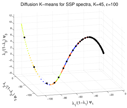
Figure 1: Diffusion $K$-means for SSP spectra. Representation of 1278 SSP spectra in 3-dimensional diffusion space. Large black dots denote the $K=45$ centroids. Individual SSPs are coloured by cluster membership. The SSPs reside on a simple, low-dimensional manifold which is captured by the $K$ prototypes.

The last step of the diffusion $K$-means algorithm is to determine the $K$ protospectra and their properties. First, the normalization constant for the $j$th prototype spectrum is

$$\widehat{\gamma}_{j}=\sum_{\mathbf{b}_{i}\in S_{j}}\frac{\phi_{0}(\mathbf{b}_{i})\gamma_{i}(\mathbf{b}_{i})}{\sum_{\mathbf{b}_{i}\in S_{j}}\phi_{0}(\mathbf{b}_{i})}$$ (8)

and the $j$th protospectrum is

$$\mathbf{\xi}_{j}=\widehat{\gamma}_{j}\sum_{\mathbf{b}_{i}\in S_{j}}\frac{\phi_{0}(\mathbf{b}_{i})\mathbf{b}_{i}}{\sum_{\mathbf{b}_{i}\in S_{j}}\phi_{0}(\mathbf{b}_{i})}$$ (9)

Similarly, the age, metallicity, and “stellar-mass fraction”—the percent of the initial stellar mass still in stars—of prototype $j$ are naturally defined as

$$t(\mathbf{\xi}_{j}) = \sum_{\mathbf{b}_{i}\in S_{j}}\frac{\phi_{0}(\mathbf{b}_{i})t(\mathbf{b}_{i})}{\sum_{\mathbf{b}_{i}\in S_{j}}\phi_{0}(\mathbf{b}_{i})}$$ (10)

$$Z(\mathbf{\xi}_{j}) = \sum_{\mathbf{b}_{i}\in S_{j}}\frac{\phi_{0}(\mathbf{b}_{i})Z(\mathbf{b}_{i})}{\sum_{\mathbf{b}_{i}\in S_{j}}\phi_{0}(\mathbf{b}_{i})}$$ (11)

$$f_{\star}(\mathbf{\xi}_{j}) = \sum_{\mathbf{b}_{i}\in S_{j}}\frac{\phi_{0}(\mathbf{b}_{i})f_{\star}(\mathbf{b}_{i})}{\sum_{\mathbf{b}_{i}\in S_{j}}\phi_{0}(\mathbf{b}_{i})}$$ (12)

where $t(\mathbf{b}_{i}),Z(\mathbf{b}_{i})$, and $f_{\star}(\mathbf{b}_{i})$ are the age, metallicity and stellar-mass fraction of the $i$th SSP, respectively. Equations (10)-(12) are natural definitions of the prototype parameters in the sense that the fit of this basis to a galaxy would yield exactly the same parameter estimates as the equivalent mixture of the original set of SSPs, $\mathbf{B}$.

In Fig. 2 we plot the 45 SSP spectra in CF05 and the 45 prototype spectra found by diffusion $K$-means. All spectra are normalized to 1 at $\lambda_{0}$=4020Å  and are coloured by log age. The diffusion $K$-means prototypes spread themselves evenly over the range of spectral profiles, capturing a gradual trend from young to old spectra. On the other hand, the CF05 basis includes many similar spectra from younger populations and sparsely covers the range of spectral profiles of older populations.

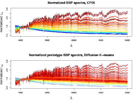
Figure 2: Basis spectra for CF05 and Diffusion $K$-means, coloured by $\log t$. All spectra are normalized to 1 at $\lambda_{0}=4020$ Å. The diffusion $K$-means basis covers the spectral range in gradual increments while the CF05 basis includes many young spectra with similar spectral properties and sparsely covers the spectral range of older populations.

See Algorithm 1 for a summary of the diffusion $K$-means algorithm. Sample Matlab and R code is available on the web at http://www.stat.cmu.edu/~annlee/software.htm. The diffusionMap R package is available at http://cran.r-project.org/.

Algorithm 1 Diffusion $K$-means

1:  Normalize SSP spectra, $\mathbf{B}$, at $\lambda_{0}$, fix $\epsilon>0$

2:  Compute similarity matrix, $\mathbf{S}$ (3) and weight matrix $\mathbf{W}$ (4)

3:  Compute $\mathbf{P}$: $p_{1}(\mathbf{b}_{i},\mathbf{b}_{j})=w(\mathbf{b}_{i},\mathbf{b}_{j})/\sum_{k}w(\mathbf{b}_{i},\mathbf{b}_{k})$

4:  Decompose $\mathbf{P}$: $p_{1}(\mathbf{b}_{i},\mathbf{b}_{j})=\sum_{k}\lambda_{k}\psi_{k}(\mathbf{b}_{i})\phi_{k}(\mathbf{b}_{j})$

5:  Project $\mathbf{B}$ to the $m$-dimensional diffusion map, $\mathbf{\Psi}$ (5)

6:  $K$-means:

7:        Set $k$=1. Fix $K$.

8:        Randomly partition data into sets $S_{1}^{(0)},...,S_{K}^{(0)}$

9:        while $S_{j}^{(k-1)}\neq S_{j}^{(k)}$ for some $j$

10:              $k=k+1$

11:              Compute cluster centroids, $\mathbf{c}(S_{j}^{(k)})$ (7)

12:              Partition the data so that

$$\mathbf{b}_{i}\in\textrm{argmin}_{S_{j}^{(k)}}||\mathbf{\Psi}(\mathbf{b}_{i})-\mathbf{c}(S_{j}^{(k)}))||_{2}^{2}$$

13:        end while

14:  return $K$ protospectra (9) and corresponding parameters (10-12)

2.2.2 Other $K$-means algorithms

In §3, we compare the fits obtained by the diffusion $K$-means basis to those found by two other numerical methods: principal components (PC) $K$-means and standard $K$-means. Each of these two methods is similar to diffusion $K$-means, but both have critical drawbacks.

PC $K$-means works similarly to diffusion $K$-means (Algorithm 1) except that $K$-means is performed on the projection of the normalized SSP spectra into principal components (PC) space, not diffusion space. For an example of the application of principal components analysis to SSP spectra see Ronen, Aragón-Salamanca & Lahav (1999). The main drawback to PC $K$-means is its assumption that the SSP spectra lie on a linear subspace of the original $p\gtrsim 10^{3}$ dimensional space. If the SSPs actually lie on a non-linear manifold, then the $K$ prototypes may poorly capture the intrinsic variation of the original SSPs because the non-linear structure will have been inappropriately collapsed on to a linear space by the principal components projection.

Standard $K$-means is also similar to Algorithm 1, except that $K$-means is performed in the original $N_{\lambda}\simeq 10^{3}$ dimensional space; i.e., no reduction in dimensionality is done before running $K$-means. There are two obvious drawbacks to this procedure. First, the algorithm generally is slow because distance computations are cumbersome in high dimensions and $K$-means usually takes more iterations to converge. For comparison, the dimensionality of the spaces used by diffusion and PC $K$-means are each $\lesssim 10$, a factor of 100 smaller than $p$. Second, and more importantly, appropriate prototype spectra are difficult to find by standard $K$-means because Euclidean distances, used by $K$-means to define clusters, are only physically meaningful over short distances. Diffusion $K$-means avoids this problem by clustering in diffusion space, in which Euclidean distance approximates diffusion distance, a measure that has physical meaning on all scales. The result is that standard $K$-means inappropriately relates SSPs that are not physically similar.

In Fig. 3, we plot $\log Z$ versus $\log t$ for $K$=150 prototypes in Asa07 and diffusion, standard, and PC $K$-means. Notably, diffusion $K$-means finds a much higher density of prototypes with high $\log Z$ or high $\log t$, reflecting the complicated manner in which SSPs with those properties vary with respect to $Z$ and $t$. At the other extreme, the Asa07 prototypes reside on a regular grid, and thus include many prototype spectra that are essentially identical and also exclude prototypes that have unique spectral properties. The standard and PC $K$-means prototypes also estimate more high $\log Z$ and high $\log t$ prototypes than a regular grid.

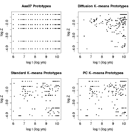
Figure 3: Plot of $\log Z$ versus $\log t$ for $K$=150 prototypes in Asa07 and $K$-means bases. There is a high density of diffusion $K$-means prototypes along a curve that encompasses large ages and metallicities. Due to the complicated manner in which those SSP spectra vary, many more prototypes are needed to span that spectral range. Contrast this to the regular grid of Asa07 prototypes.

2.2.3 Incorporating other information

The methods introduced above use only the observable properties of SSPs to choose representative prototypes. It may be the case that we want to incorporate other a priori information that we have about the SSPs and their relationship with the galaxies we are fitting. For instance, we might know that a SSP with a particular age and metallicity is generally found in the types of galaxies we are trying to fit, and hence will want to include in our basis a prototype with characteristics closely matching those of this SSP. This information can easily be incorporated with the framework introduced above by defining an a priori weight, $w_{i}\geq 0$ for each SSP in our database, where higher weights signify more importance of the SSP.

By modifying the definition of the diffusion map geometric centroid (7) to be

$$\mathbf{c}_{w}(S_{j})=\sum_{i:\mathbf{b}_{i}\in S_{j}}\frac{w_{i}\phi_{0}(\mathbf{b}_{i})\mathbf{\Psi}(\mathbf{b}_{i})}{\sum_{\mathbf{b}_{i}\in S_{j}}w_{i}\phi_{0}(\mathbf{b}_{i})},$$ (13)

and altering the $K$-means algorithm to minimize

$$V_{w}=\sum_{j=1}^{K}\sum_{i:\mathbf{b}_{i}\in S_{j}}w_{i}||\mathbf{\Psi}(\mathbf{b}_{i})-\mathbf{c}_{w}(S_{j})||_{2}^{2}$$ (14)

instead of $V$ in (6), we choose a basis that reflects both the numerical observable properties of the SSPs and our a priori knowledge.

This weighted $K$-means algorithm can be used to correct for the tendency of the prototype SSPs to depend on the specific set of SSPs, $\mathbf{B}$, chosen. If, for example, we define $w_{i}$ as the inverse of the local density of SSP $i$, then the prototype SSPs in Fig. 1 would more uniformly cover the manifold of SSPs in diffusion space, and not tend to more heavily sample denser regions of the SSP manifold. In this manner, the prototype spectra will only depend on the spectral properties, and not the particular sampling of the set of SSPs.

3 Simulations

We use simulations to assess the performance of the diffusion $K$-means method for selection of a basis of prototype SSP spectra compared to bases derived by other $K$-means methods and the bases of $K=45$ used by CF05 and $K=150$ used by Asa07. We analyse the performance of these methods on physically-motivated simulated spectra from two different prescriptions. All simulated galaxy spectra are generated as mixtures of a fine grid of 1278 SSP spectra from the model of Bruzual & Charlot (2003), as described in §2.1.2. We construct the simulated spectra with a fine grid of SSPs because we expect real galaxies to consist of sub-populations of stars on a continuous grid of age and $Z$. This approach differs significantly from the simulation prescriptions of, for example, Cid Fernandes et al. (2004) and Cid Fernandes et al. (2005) as discussed in §2.1.2.

Like Cid Fernandes et al. (2005), we simulate spectra over the range 3650-8000 Å. We bin all spectra to one measurement every 1 Å. For each simulated galaxy, we independently sample the reddening parameter, $A_{V}$, and velocity dispersion, $\sigma_{*}$, from a realistic distribution based on fits to a large sample of SDSS galaxies by the STARLIGHT code that was performed by the SEAGal (Semi Empirical Analysis of Galaxies) Group and is available on the web at www.starlight.ufsc.br. We add Gaussian noise following the normalized mean SDSS error spectrum with specified S/N at $\lambda_{0}=4020$ Å. We mask out any spectral bins around emission lines, as done in Cid Fernandes et al. (2005).

To choose the optimal value of $\epsilon$ for the diffusion $K$-means basis, we fit simulations to each basis from a grid of $\epsilon$ values and find the basis for which the fits achieve the smallest median $\chi^{2}$ value, (2). Although we choose the optimal $\epsilon$ by minimizing $\chi^{2}$, our ultimate goal is accurate estimation of the SFH and physical parameters for each galaxy. However, we find that bases that achieve small $\chi^{2}$ values tend to have small errors in their physical parameter estimates.

To compare results across different bases, we compare the errors in physical parameter and SFH estimation. Our ultimate goal is to find the basis that most accurately describes the star formation and metallicity history of each galaxy. In this study, our main parameters of interest are

$$\langle\log t\rangle_{L} = \sum_{j=1}^{K}x_{j}\log(t(\xi_{j})),$$ (15)

$$\log\langle Z\rangle_{L} = \log\left(\sum_{j=1}^{K}x_{j}Z(\xi_{j})\right),$$ (16)

$A_{V}$, and $\sigma_{*}$. To test the ability of different bases to estimate these parameters, we compute the mean square error (MSE) of the estimates across the simulated galaxies. To characterize the ability to recover SFH, we compute condensed population vectors by binning both $\mathbf{x}$ and $\mathbf{\mu}$ into 5 logarithmically spaced time bins and then comparing these true condensed vectors, $\mathbf{x}_{c}$ and $\mathbf{\mu}_{c}$ to the estimated condensed vectors, $\mathbf{\widehat{x}}_{c}$ and $\mathbf{\widehat{\mu}}_{c}$. Other techniques have proposed different schemes for compressing the SFH information retrieved by spectral fitting (see Asari et al. 2007 for an overview of the different compression methods employed in current spectral synthesis codes). Our choice of 5 age bins is an attempt to avoid the degeneracies that are likely if the population vector were gridded into very fine age bins while still retaining a sufficient number of age bins to detect significant recent starburst events. Admittedly, the choice of 5 age bins is ad hoc. However, because we are only interested in comparing the ability of different bases of prototype spectra to recover SFH, any reasonable parametrization of the SFH will allow us to perform this analysis.

3.1 Exponentially decreasing SFH

In the first set of simulations, we choose a SFH with exponentially decaying star formation rate (SFR): SFR $\propto\exp(\gamma t)$, where $t$ is the age of the SSP in Gyr and we use SSPs up to a maximum of 14 Gyrs. Like Tojeiro et al. (2007), we set $\gamma=0.3\textrm{Gyr}^{-1}$ to have a SFH that is neither dominated by recent star formation nor too similar to a single old burst galaxy. In our simulations, we consider specific SFR (SSFR) as defined in Asari et al. (2007) by normalizing all simulated spectra to have the same mass. This is reasonable because in practice we are interested in how the SFH varies across many galaxies, and therefore wish to remove the absolute mass-scale dependence of each object’s SFR. We have SSPs from 196 time bins where each bin’s metallicity is randomly chosen from 6 different values. We test our methods on 50 simulated spectra. Across different spectra the SFH is the same, while $\log\langle Z_{*}\rangle_{L},A_{V},\sigma_{*}$ and the random noise all vary. Each spectrum has S/N=10 at $\lambda_{0}$.

3.1.1 Results

The following bases of prototype spectra are used to fit each simulated spectrum: 1) the CF05 basis, 2) diffusion $K$-means, 3) PC $K$-means, and 4) standard $K$-means. Each basis contains $K=45$ prototype spectra. For diffusion $K$-means, we perform fits over a grid of values of $\epsilon$ to study how parameter estimates vary as a function of $\epsilon$.

In Fig. 4 we show the error in spectral fits using diffusion $K$-means for different values of $\epsilon$. Also plotted is the error in the standard $K$-means (sK) and PC $K$-means (PC) bases. All errors are plotted as the ratio of the $\chi^{2}$ statistic to the $\chi^{2}$ from the CF05 basis fit. In the vast majority of the simulated spectra, all three of the techniques considered produce better spectral fits than the CF05 basis. There are no significant differences between spectral fit errors for the diffusion $K$-means bases as $\epsilon$ varies. The minimum median $\chi^{2}$ for diffusion $K$-means is achieved at $\epsilon=750$.

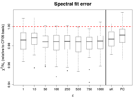
Figure 4: Spectral fit errors to simulated spectra with exponentially decreasing SFH, $\gamma=0.3$. Errors are plotted relative to the error obtained by the CF05 basis (dashed line). For each value of $\epsilon$, diffusion $K$-means outperforms the CF05 basis, as do both standard $K$-means (sK) and PC $K$-means (PC).

We plot the MSE of our estimates for $\langle\log t_{*}\rangle_{L},\log\langle Z_{*}\rangle_{L},A_{V}$, and $\sigma_{*}$ in Fig. 5. For each parameter, the CF05 basis predictions are the worst in terms of MSE. The performance of the diffusion $K$-means basis is not very dependent on the particular choice of $\epsilon$. This is a nice property, as any reasonable choice of $\epsilon$ will give us good results, and we need not spend computing time searching for an optimal value of $\epsilon$. Diffusion $K$-means bases tend to find the best estimates of $\langle\log t_{*}\rangle_{L}$, $A_{V}$, and $\sigma_{*}$, and performs competitively with the other $K$-means bases for $\log\langle Z_{*}\rangle_{L}$ estimation.

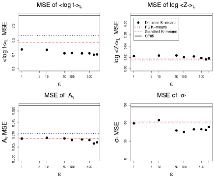
Figure 5: MSE of four parameter estimates, for simulated spectra with exponentially-decaying SFH, $\gamma=0.3$. MSE is computed across 50 simulated spectra with S/N=10. Parameter estimates from the diffusion $K$-means bases (solid dots) are plotted along with those from the CF05 basis (solid line), standard $K$-means basis (dashed line), and PC $K$-means basis (dotted line). The diffusion $K$-means basis generally outperforms the other bases considered; CF05 estimates poorly for all 4 parameters.

We compare the condensed SFH estimates across bases. Plots of the recovered $\mathbf{\widehat{x}}_{c}$ and $\mathbf{\widehat{\mu}}_{c}$ vectors in Fig. 6 show that the CF05 basis tends to significantly underestimate the contributions of the oldest population while overestimating the contribution of the second oldest population. All three $K$-means bases find estimates that are closer to the true $\mathbf{\widehat{x}}_{c}$, but tend to underestimate the contribution of the oldest $\mathbf{\widehat{x}}_{c}$ component. All three $K$-means bases find very accurate estimates of $\mathbf{\widehat{\mu}}_{c}$. The bias in $\mathbf{\widehat{x}}_{c}$ estimation occurs for at least two reasons. First, since the simulations are generated from SSPs on a fine age grid, it is intrinsically difficult to estimate all of the contributions of the subpopulations. Second, due to the exponential form of the SFR, older populations are the most important in the SFH, making it easy to underestimate their importance and almost impossible to overestimate their contribution.

Figure 6: Estimated star formation histories for simulated spectra with exponentially-decaying SFH, $\gamma=0.3$. The estimated SFHs for 4 different bases are plotted as dots with dashed lines to denote the median estimated contribution of galaxy light (left column) and galaxy mass (right column) formed in each time bin for fits to 50 simulations. Error bars denote the 90% prediction intervals for the fits. The true, underlying model, SFR $\propto\exp(\gamma t)$, is plotted as a solid line. The CF05 basis performs much worse than the $K$-means bases, confusing old populations for younger ones.

For this simple prescription of galaxy evolution, bases constructed using $K$-means methods find significantly better estimates of physical parameters and SFH than the CF05 basis. Next, we test our methods on a slightly more complicated set of simulations and also compare bases of size 45 and 150 to characterize the advantage, if any, of using a larger basis and whether this advantage is worth the extra expenditure in computation time.

3.2 Exponentially decreasing SFH with random starbursts

In our second set of simulations, we use a prescription similar to Chen et al. (2009) to create a set of more realistic spectra on which to test our methods. The added SFH complexities over the simulations in §3.1 are:

1. The time $t_{form}$ when a galaxy begins star formation is distributed uniformly between 0 and 5.7 Gyr after the Big Bang, where the Universe is assumed to be 13.7 Gyr old.

2. We again have SFR $\propto\exp(\gamma t)$, but now allow $\gamma$ to vary between galaxies. For each galaxy we draw $\gamma$ from a uniform distribution between 0.7 and 1 $\textrm{Gyr}^{-1}$.

3. We allow for starbursts with equal probability at all times. The probability a starburst begins at time $t$ is normalized so that the probability of no starbursts in the life of the galaxy is 33%. The length of each burst is distributed uniformly between 0.03 and 0.3 Gyr and the fraction of total stellar mass formed in the burst in the past 0.5 Gyr is distributed logarithmically between 0 and 0.1. The SFR of each starburst is constant throughout the length of the burst.

As above, each galaxy spectrum is generated as a mixture of SSPs of up to 196 time bins, with a randomly drawn metallicity in each bin. Allowing for random starbursts over the exponential SFH increases the importance of younger populations in the simulated galaxies. We test our methods on 500 simulated spectra, 250 with S/N=10 and 250 with S/N=20 at $\lambda_{0}$. Across each spectrum, SFH, $\log\langle Z\rangle_{L},A_{V},\sigma_{*}$ and the random noise all vary. We fit bases of size 45 and 150.

3.2.1 Results

For this set of simulations, we only look at results for the diffusion $K$-means $\epsilon$ that achieves the lowest $\chi^{2}$ fit error for each $K$; the optimal values are $\epsilon$=250 for the $K=45$ basis and $\epsilon$=500 for the $K=150$ basis. As before, results are not very sensitive to the specific choice of $\epsilon$. Note that the $\epsilon$=250 basis of size 45 also achieved good fits to the simpler simulations in §3.1. In Fig. 7 we plot the MSE of the physical parameter estimates for each of the 4 bases for $K$=45 and 150. The diffusion $K$-means bases perform significantly better than all other bases for mean age and $A_{V}$ estimation and achieve similar results as the other $K$-means bases for $\log\langle Z_{*}\rangle_{L}$ and $\sigma_{*}$ estimation. The $K$-means bases heavily outperform the hand-chosen bases (CF05 & Asa07) for each parameter. The same trends are seen for error in estimation of time-binned star formation histories (Fig. 8). The error estimates for all bases, split into S/N=10 and S/N=20 galaxy spectra, are in Table 1.

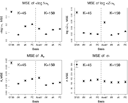
Figure 7: MSE of four parameter estimates for simulated spectra with exponentially decreasing SFH and random starbursts. Plotted for each basis is the MSE plus standard error across 500 simulations. The $K$-means bases outperform bases from the literature for both choices of $K$. Diffusion $K$-means tends to find the best parameter estimates, showing no significant change in accuracy between $K$=45 and 150.

Figure 8: Error in SFH estimation for simulated spectra with exponentially decreasing SFH and random starbursts. Average discrepancies of the estimated condensed light fraction ($\mathbf{\widehat{x}}_{c}$) and condensed mass fraction ($\mathbf{\widehat{\mu}}_{c}$) vectors to the truth, averaged across 500 simulations. Diffusion $K$-means generally produces more accurate SFH estimates than the other bases considered. All $K$-means bases find much more accurate estimates than the literature bases.

Table 1: Summary of parameter error estimates for simulated spectra with exponentially decreasing SFH and random starbursts.

		S/N=10						S/N=20
$K$	Basis	$\langle\log t_{*}\rangle_{L}$	$\log\langle Z_{*}\rangle_{L}$	$A_{V}$	$\sigma_{*}$	$\mathbf{x}_{c}$	$\mathbf{\mu}_{c}$	$\langle\log t_{*}\rangle_{L}$	$\log\langle Z_{*}\rangle_{L}$	$A_{V}$	$\sigma_{*}$	$\mathbf{x}_{c}$	$\mathbf{\mu}_{c}$
	CF05	0.368	0.089	0.025	369.0	0.664	0.349	0.360	0.089	0.022	229.6	0.675	0.333
45	dM	0.074	0.024	0.007	156.4	0.195	0.059	0.074	0.025	0.007	93.3	0.213	0.059
	sK	0.194	0.021	0.010	171.7	0.219	0.046	0.169	0.022	0.009	97.3	0.191	0.030
	PC	0.222	0.020	0.012	174.6	0.212	0.046	0.193	0.020	0.010	107.6	0.187	0.029
	Asa07	0.167	0.059	0.013	169.6	0.421	0.175	0.134	0.056	0.010	77.4	0.390	0.150
150	dM	0.093	0.018	0.007	153.1	0.213	0.067	0.068	0.018	0.005	70.1	0.182	0.050
	sK	0.150	0.021	0.008	153.4	0.303	0.118	0.124	0.020	0.007	69.5	0.292	0.105
	PC	0.163	0.029	0.009	160.9	0.317	0.117	0.130	0.029	0.007	71.1	0.301	0.099

An interesting trend appears in Figs. 7-8. For the hand-chosen bases, we see considerable reduction in the estimation error of every parameter in going from the $K$=45 basis of CF05 to the $K$=150 basis of Asa07. However, in the $K$-means bases, and particularly for the diffusion $K$-means basis, there is no substantial lowering of the MSE of any parameter in increasing from $K$=45 to $K$=150. This tells us that even with as few as 45 prototypes, diffusion $K$-means provides us a basis that can successfully fit these particular simulations. Moving to $K$=150 prototypes allows us no significant gains in parameter estimation while costing us $\sim$10 times the computational time. Note, however, that although a basis of size 45 may be sufficient for this set of simulations, a set of real galaxy spectra may be more complicated and require a larger basis of prototypes to achieve good fits.

A common difficulty in population synthesis studies is the so-called age-metallicity degeneracy, where young, metal-rich SSPs are confused with old, metal-poor SSPs. Using a regular grid of SSP prototypes in population synthesis can exacerbate this problem because several SSPs with nearly identical spectra (but different ages and metallicities) will likely be included, inducing degeneracy in the spectral model (1), and causing the estimated SFH parameters for each galaxy to be highly variable. A diffusion $K$-means basis, on the other hand, picks SSP prototypes whose spectra more evenly span the range of spectral characteristics, minimizing the inclusion of very similar spectra and thus decreasing the degeneracy effects in the minimization of (2). In Fig. 9 we see that the age-Z degeneracy is much smaller in diffusion $K$-means bases, quantified by the slope of the linear trend in $\Delta\log\langle Z_{*}\rangle_{L}$ versus $\Delta\langle\log t_{*}\rangle_{L}$. Some degeneracy in age-metallicity still exists for the diffusion $K$-means bases, but the magnitude of the slope of the trend is half.

One may note that both $\log\langle Z_{*}\rangle_{L}$ and $\langle\log t_{*}\rangle_{L}$ are significantly biased for all 4 bases in Fig. 9. This probably occurs due to the simulation prescription, which includes mostly old SSPs from a large, fine grid of age and Z. One may be inclined to use these estimated biases to correct the estimates of real galaxy spectra. However, the amount of bias is dependent on the particular prescription of SFH in the simulations. Since there is no general model that describes galaxy SFH for a wide range of galaxies, there is no straightforward way to estimate the bias, if any, that will occur.

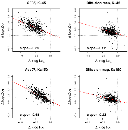
Figure 9: Age-metallicity degeneracy in parameter estimation for simulated spectra with exponentially decreasing SFH and random starbursts. Diffusion $K$-means bases show significantly less degeneracy in parameter estimates than the literature bases, shown by a smaller slope in the linear trend. Diffusion $K$-means bases also produce less biased estimates of both parameters.

4 Application to SDSS spectra

In this section, we apply the fitting techniques to a sample of SDSS spectra to compare the results using different bases. We compare the physical parameters estimated from each of three different bases: Asa07, diffusion map with $K$=45, and diffusion map with $K$=150. We also compare parameter estimates to those estimated with the MPA/JHU data base. Our goal in this section is to study how the choice of basis affects the final parameter estimates for a large set of real galaxy spectra.

4.1 Data preparation

Our data sample consists of spectra from ten arbitrarily chosen spectroscopic plates of SDSS DR6 (0266$-$0274 inclusive, and 0286; Adelman-McCarthy et al. 2008) that are classified as galaxy spectra. The goal is to test our methods on a sample that is large enough that we include galaxies with a broad range of star formation and metallicity histories but not so large that analysis is computationally cumbersome. In a future work, we will present results for the more than 700k galaxy spectra in SDSS DR7.

We remove spectra from this sample by applying three cuts. The first, motivated by aperture considerations, is to analyse only spectra whose SDSS redshift estimates $\geq$ 0.05. Second, we determine the proportion of the 3850 wavelength bins that are flagged as bad. If this proportion exceeds 10%, we remove the spectrum from the sample; if not, we retain the spectrum for further analysis. Third, we select galaxy spectra with a SDSS redshift confidence level $\geq$ 0.35. These cuts leave us with a sample of 3046 galaxy spectra.

We bring all spectra to rest frame using the SDSS redshift estimates. In the fitting routines, we exclude any spectral bins with SDSS flag $\geq$ 2. This eliminates any sky residuals, bad pixels, and artefacts from the data reduction. We additionally mask the pixels in the regions within and around emission lines as in Cid Fernandes et al. (2005). Results of the STARLIGHT spectral fits give a mean $\chi^{2}/N_{\lambda}$ of 1.03 for each of the three bases used, close to a value of 1 that would be expected if wavelength bin fluxes were independently distributed Gaussian random variables. Note that this value varies considerably from the mean value of 0.78 found in the analysis of 50362 SDSS spectra by Cid Fernandes et al. (2005). This difference can be attributed to our careful handling of spectral bin error estimates in our rebinning of the spectra to a dispersion of 1 measurement per Å.

4.2 Parameter estimates

The STARLIGHT fitting routine is used to fit all 3046 SDSS spectra with each of the three bases. Each basis yields parameter estimates that are substantially different. In Fig. 10 we plot each galaxy’s $\log\langle Z_{*}\rangle_{L}$ versus $\langle\log t_{*}\rangle_{L}$ estimate for each basis. There are several notable differences in the $\log\langle Z_{*}\rangle_{L}-\langle\log t_{*}\rangle_{L}$ plane for each basis. First, both diffusion map bases produce estimates that are tightly centered around an increasing linear trend while the Asa07 estimates are diffusely spread around such a trend. Moreover, the direction of discrepancy in the Asa07 estimates from the linear trend corresponds exactly with the direction of degeneracy between old, metal-poor and young, metal-rich galaxies. This suggests that the observed variability along this direction is not due to the physics of these galaxies, but rather is caused by confusion stemming from the choice of basis.

Secondly, the slopes of the estimated trends produced by the diffusion map bases (0.146 for $K$=45 and 0.180 for $K$=150) are considerably smaller than the slope of the trend in the Asa07 estimates (0.250). These estimates have implications for the physical models that govern galaxy evolution. Finally, the $K$=45 diffusion map basis estimates no young, metal-poor galaxies, showing a sharp decline from densely-populated regions of the parameter space to vacant regions. This suggests that this small number of prototypes is not sufficient to cover the parameter space; particularly, young, metal-poor SSPs have been neglected in the basis.

Figure 10: Estimated ages and metallicities for 3046 SDSS galaxies. Diffusion $K$-means estimates tend to lie tightly around a linear trend in this plane while Asa07 estimates show large dispersion in the perpendicular direction, which corresponds to the direction of age-Z degeneracy in galaxy population synthesis studies.

Next we compare kinematic parameter estimation. Fig. 11 shows that the Asa07 basis tends to consistently estimate slightly larger values of $A_{V}$ than either diffusion map basis. On average, Asa07 estimates of $A_{V}$ are 0.045 larger than diffusion map $K$=45 estimates and 0.024 larger than diffusion map $K$=150 estimates. Estimates of $\sigma_{*}$ are consistent between all three bases.

Finally, we compare age-binned SFH estimates found by each basis. Like Cid Fernandes et al. (2005), we condense the SFH to three parameters: old, $x_{\textrm{o}}$ ($t_{j}>10^{9}$ yr), intermediate, $x_{\textrm{i}}$ ($10^{8}\leq t_{j}\leq 10^{9}$ yr), and young, $x_{\textrm{y}}$ ($t_{j}<10^{8}$ yr). Plots of diffusion map estimates of each component versus Asa07 estimates are in Fig. 12. The estimated SFHs show a high degree of correspondence between the bases. On average, each diffusion map basis obtains slightly higher estimates of $x_{\textrm{o}}$ and slightly lower estimates of both $x_{\textrm{i}}$ and $x_{\textrm{y}}$.

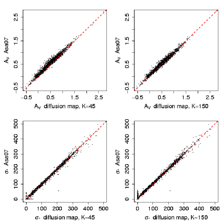
Figure 11: Estimated $A_{V}$ and $\sigma_{*}$ parameters for 3046 SDSS galaxies. The Asa07 $A_{V}$ estimates tend to be larger than the corresponding diffusion map estimates. The $\sigma_{*}$ estimates agree for all 3 bases.

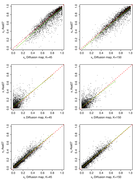
Figure 12: Age-binned population vector for 3046 SDSS galaxies. Plotted are the Asa07 estimates of the 3-dimensional age-binned population vector versus those of two diffusion $K$-means bases. Diffusion map tends to find slightly smaller contributions of the oldest populations.

4.3 Comparisons to the MPA/JHU data base

We compare the SDSS parameters estimated with the three different choices of STARLIGHT basis with parameters obtained using measured emission line and continua values from the MPA/JHU data base. The MPA/JHU collaboration has made their SDSS spectral measurements publicly available on the MPA SDSS website (Kauffmann et al. 2003; Brinchmann et al. 2004; Tremonti et al. 2004). Although we do not expect any of the basis choices to produce estimates that perfectly correspond to the independent MPA/JHU estimates, we analyse the relationships between the estimates as a further test of the accuracy of each basis.

4.3.1 $A_{V}$ and $A_{V}^{\rm neb}$

We use the Balmer emission-line ratio $H\alpha/H\beta$ to estimate the nebular extinction, $A_{V}^{\rm neb}$ , of each galaxy. Following Osterbrock (1989), we assume case B recombination, a density of 100 cm^-3 and a temperature of 10⁴ K to compute $A_{V}^{\rm neb}$ according to (17)-(18):

$$A_{V}^{\rm neb} = c\times 3.1/1.47$$ (17)

$$c = -2.70(2.86-\log(H\alpha/H\beta)_{\rm obs})$$ (18)

where we have used the same constants used in Chen et al. (2009).

Fig. 13 shows plots of the values of $A_{V}^{\rm neb}$ computed from the MPA/JHU data base versus the values of the stellar extinction, $A_{V}$, computed by each of the three different bases in the STARLIGHT code. We have only plotted the 1755 SDSS galaxies in our sample whose $H\alpha$ and $H\beta$ emission line measurements both have signal-to-noise ratio $\geq 3$. We find that $A_{V}^{\rm neb}$ and $A_{V}$ are loosely linearly related for each basis. The estimated Spearman correlation is 0.51 for the Asa07 basis and 0.52 for each diffusion map basis. The slope of the linear trend is slightly higher for the Asa07 basis (1.21) than for the diffusion map bases (1.16 for each basis). All three bases obtain stellar extinction estimates that are consistent with the nebular extinction values $A_{V}^{\rm neb}$, and there are no significant differences between the strength of the relationships between the estimates of each basis and the nebular extinction estimates.

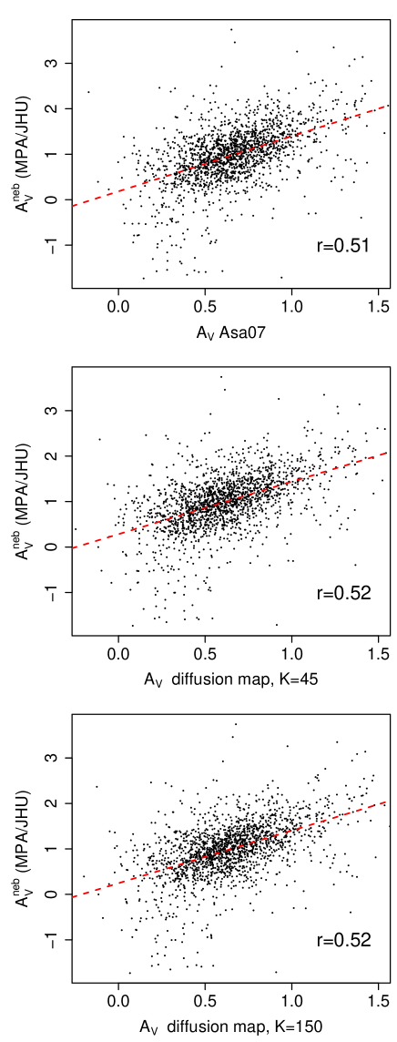
Figure 13: MPA/JHU versus population synthesis reddening estimates for SDSS galaxies. All three bases considered find estimates that are generally consistent with the independent MPA/JHU emission line estimates.

4.3.2 $\langle\log t_{*}\rangle_{L}$ and $D_{n}(4000)$ & $H\delta_{A}$

As in Chen et al. (2009), we compare our spectral synthesis estimates to two age indicators from the MPA/JHU database: $D_{n}(4000)$ (Balogh et al. 1999) and $H\delta_{A}$ (Worthey & Ottaviani 1997). The value $D_{n}(4000)$ describes the break in the 4000 Å  region of the galaxy spectrum; higher values generally correspond to increasing ages of the galaxy’s stellar subpopulations. Larger strength of the $H\delta$ absorption line, $H\delta_{A}$, indicates higher star formation rates in the past 0.1-1 Gyr of a galaxy’s lifetime. Hence, we expect our estimates of $\langle\log t_{*}\rangle_{L}$ to correlate positively with $D_{n}(4000)$ and negatively with $H\delta_{A}$.

In Fig. 14, we see that the $\langle\log t_{*}\rangle_{L}$ estimates show the expected relationships with both $D_{n}(4000)$ and $H\delta_{A}$ for each of the three bases. Correlations are strongly positive for the $D_{n}(4000)-\langle\log t_{*}\rangle_{L}$ trend and strongly negative for the $H\delta_{A}-\langle\log t_{*}\rangle_{L}$ trend. We have plotted the 3031 galaxies in our sample that have reliable $D_{n}(4000)$ and $H\delta_{A}$ measurements in the MPA/JHU catalogue. There is no significant difference in each relation between the bases.

Figure 14: MPA/JHU versus population synthesis age indicators for SDSS galaxies. All three bases considered retrieve estimates that are consistent with two different MPA/JHU indicators of age of stellar population.

4.3.3 $\langle Z_{*}\rangle_{M}$ and $Z_{\rm neb}^{\rm o3n2}$

Lastly, we compare our STARLIGHT estimates of $\langle Z_{*}\rangle_{M}$ with a measure of nebular metallicity based on the ratio of emission lines [OIII]$\lambda 5007$ and [NII]$\lambda 6583$, provided by MPA/JHU. Particularly, the quantity $Z_{\rm neb}$ measures the oxygen abundance of a galaxy, and is defined as

$$Z_{\rm neb}=-3.45-.25\times{\rm O}_{3}{\rm N}_{2}$$ (19)

where O₃N${}_{2}=\log([{\rm OIII}]\lambda 5007/[{\rm NII}]\lambda 6583)$ (Pettini & Pagel 2004). All emission line fluxes are first corrected for extinction using the $A_{V}$ estimates found in STARLIGHT fits. We would expect $\langle Z_{*}\rangle_{M}$ to be positively related to $Z_{\rm neb}$, as the former measures stellar metallicity and the latter measures nebular oxygen abundance.

In Fig. 15 we see that all three bases find $\langle Z_{*}\rangle_{M}$ estimates that correlate positively with $Z_{\rm neb}$, and that the $Z$=150 diffusion map basis estimates correlate more strongly with $Z_{\rm neb}$, with Spearman correlation coefficient of 0.21, compared to the Asa07 basis estimates, which have a correlation of 0.12 with the $Z_{\rm neb}$ estimates. Furthermore, the best-fit linear trend of the $Z_{\rm neb}$ versus diffusion map $K$=150 estimates has a significantly higher slope, 0.128 than the linear trend of $Z_{\rm neb}$ vs. Asa07 basis, 0.056. This result suggests that the diffusion map basis obtains more reliable metallicity estimates than the Asa07 basis.

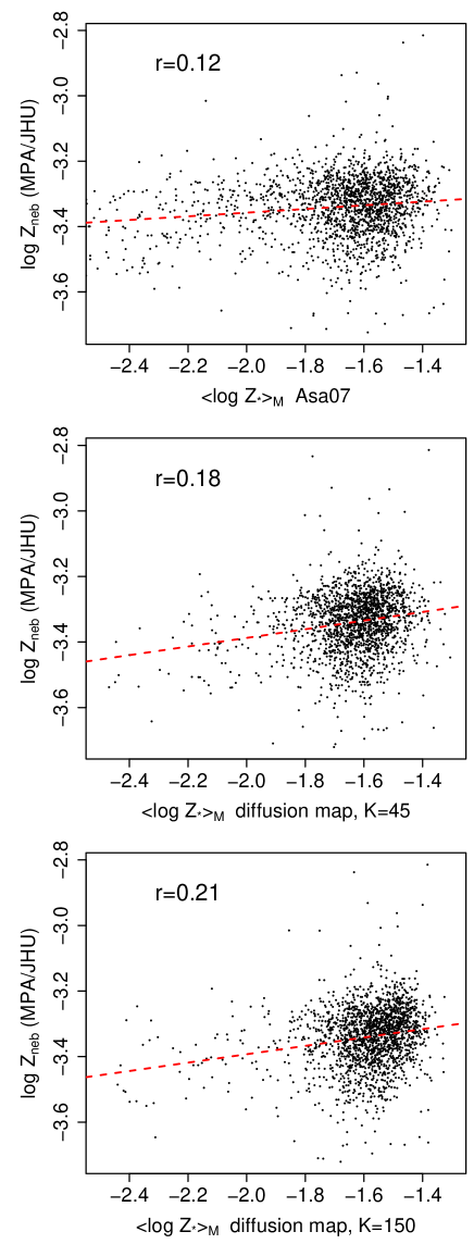
Figure 15: MPA/JHU versus population synthesis metallicity estimates for SDSS galaxies. MPA/JHU estimates of nebular oxygen abundance correlate more strongly with diffusion $K$-means estimates of stellar metallicity than the Asa07 estimates.

5 Discussion

We have presented a method to choose an appropriate basis of SSP prototypes to be used in population synthesis models of observed galaxy spectra. Particularly, we have used the STARLIGHT fitting routines of Cid Fernandes et al. (2005) to study the ability of both literature and diffusion $K$-means bases to model both simulated and SDSS galaxy spectra. On simulated galaxies, our diffusion $K$-means basis outperforms hand-chosen literature bases as well as bases constructed from standard $K$-means or PC $K$-means. For real SDSS galaxy spectra, we show that the diffusion $K$-means basis finds parameter estimates that differ substantially from the estimates retrieved by the basis of Asari et al. (2007). The diffusion $K$-means estimates seem to alleviate the age-metallicity degeneracy that has been detrimental to previous population synthesis studies of large data bases of galaxies.

At this point, more discussion of the age-metallicity degeneracy is warranted. Degeneracy arises because several SSPs have very similar spectral characteristics, but different ages and metallicities. When degenerate SSPs are included, estimates can be highly variable. This is shown in the first panel in Fig. 10 and in the STARLIGHT code itself, which in the presence of degeneracy tends to converge to different solutions due to the random walk taken through the parameter space by the Metropolis algorithm. The diffusion $K$-means algorithm, on the other hand, includes only the mean spectrum and mean parameters of each set of degenerate spectra. This choice minimizes the statistical risk of the final solution by decreasing the variance and bias of the estimates (our measure of statistical risk is the MSE, which is the sum of the variance and squared bias of an estimate), as seen in simulations (Figs. 5-9). Our SFH estimates for SDSS spectra are significantly less variable in the direction of the age-Z degeneracy, as seen in Fig. 10, while the relative amount of bias is impossible to quantify without knowledge of the true SFH of each galaxy.

In the face of degeneracies and with no other outside information available, our proposed method (of picking the mean of several degenerate solutions) is the best one can do in terms of minimizing the statistical risk of the estimates. However, with more information about what features in the SSP spectra are most strongly related to their ages and metallicities, we could potentially improve our estimates by incorporating such information in the construction of the similarity measure $s(\mathbf{b}_{i},\mathbf{b}_{j})$ in (3). The weight matrix produced by an expert-produced similarity measure may produce a more complete coverage of the parameter space in our SSP prototypes and help to remove degeneracies in the parameter estimates. Further study is required in this direction.

The ultimate goal of this project is to be able to quickly and accurately estimate physical property and SFH parameters for a large data base of galaxies. As an extension of this work, we plan to study how to quickly and effectively extend estimates found for a small set of galaxies using the computationally intensive STARLIGHT routine to a large database of galaxies. To achieve this goal, we must exploit the low-dimensional structure of these data. This approach was taken by Richards et al. (2009) in galaxy redshift estimation. These methods must be further developed and refined to reliably estimate SFH parameters.

The methods presented in this paper are applicable in a wide range of problems in astrophysical data analysis. Diffusion map is a powerful tool to uncover simple structure in complicated, high-dimensional data, whether they be spectra, photometric colours, two-dimensional images, data cubes, etc. Specifically, diffusion map is both more flexible and more widely applicable than PCA, which relies on the linear correlation structure of the data and assumes that the data reside on a low-dimensional, linear manifold. The diffusion $K$-means method can be used in a variety of problems often encountered in astrophysics where a large set of observed or model data are described with a few prototype examples.

Future work will attempt to more concretely define criteria for the performance of algorithms that define $K$ prototypes from $N$ data points and to theoretically justify the use of diffusion $K$-means. We plan to explore more deeply the relationship between the $K$-means methods introduced here and to compare the methods introduced in this paper to other methods of basis selection, such as Basis Pursuit and Matching Pursuit. We also will investigate how meaningful standard errors can be attached to our parameter estimates using any choice of basis.

References

- Adelman-McCarthy et al. (2008) Adelman-McCarthy, J. K., et al. 2008, ApJS, 175, 297
- Alongi et al. (1993) Alongi, M., Bertelli, G., Bressan, A., Chiosi, C., Fagotto, F., Greggio, L., and Nasi, E., 1993, A&AS, 97, 851
- Asari et al. (2007) Asari, N. V., Cid Fernandes, R., Stasińska, G., Torres-Papaqui, J. P., Mateus, A., Sodré, L., Schoenell, W., and Gomes, J. M., 2007, MNRAS, 381, 263
- Balogh et al. (1999) Balogh, M. L., Morris, S. L., Yee, H. K. C., Carlberg, R. G. and Ellingson, E., 1999, ApJ, 527, 54
- Bica (1988) Bica, E., 1988, A&A, 195, 76
- Bressan et al. (1993) Bressan, A., Fagotto, F., Bertelli, G., Chiosi, C., 1993, A&AS, 100, 647
- Brinchmann et al. (2004) Brinchmann, J., Charlot, S., White, S. D. M., Tremonti, C., Kauffmann, G., Heckman, T., and Brinkmann, J., 2004, MNRAS, 351, 1151
- Bruzual & Charlot (2003) Bruzual, G., and Charlot, S., 2003, MNRAS, 344, 1000
- Cardelli, Clayton & Mathis (1989) Cardelli, J. A., Clayton, G. C., and Mathis, J. S., 1989, ApJ, 345, 245
- Chabrier (2003) Chabrier, G., 2003, PASP, 115, 763
- Chen et al. (2009) Chen, X. Y., Liang, Y. C., Hammer, F., Zhao, Y. H. and Zhong, G. H., 2009, A&A, 495, 457
- Cid Fernandes et al. (2001) Cid Fernandes, R., Sodre, L., Schmitt, H. R., Leao, J. R. S., 2001, MNRAS, 325, 60
- Cid Fernandes et al. (2004) Cid Fernandes, R., Gu, Q., Melnick, J., Terlevich, E., Terlevich, R., Kunth, D., Rodrigues Lacerda, R., and Joguet, B., 2004, MNRAS, 355, 273
- Cid Fernandes et al. (2005) Cid Fernandes, R., Mateus, A., Sodré, L., Stasińska, G., and Gomes, J. M., 2005, MNRAS, 358, 363
- Coifman & Lafon (2006) Coifman, R. R., & Lafon, S., 2006, Appl. Comput. Harmon. Anal., 21, 5
- Fagotto et al. (1994a) Fagotto, F., Bressan, A., Bertelli, G., Chiosi, C., 1994a, A&AS, 104, 365
- Fagotto et al. (1994b) Fagotto, F., Bressan, A., Bertelli, G., Chiosi, C., 1994b, A&AS, 105, 29
- Freeman et al. (2009) Freeman, P. E., Newman, J. A., Lee, A. B., Richards, J. W., and Schafer, C. M., in preparation.
- Gallazzi et al. (2005) Gallazzi, A., Charlot, S., Brinchmann, J., White, S. D. M., and Tremonti, C. A., 2005, MNRAS, 362, 41
- Girardi et al. (1996) Girardi, L., Bressan, A., Chiosi, C., Bertelli, G., and Nasi, E., 1996, A&AS, 117, 113
- Glazebrook et al. (2003) Glazebrook, K., et al., 2003, ApJ, 587, 55
- Kauffmann et al. (2003) Kauffmann, G. et al., 2003, MNRAS, 341, 33
- Lafon & Lee (2006) Lafon, S., & Lee, A., 2006, IEEE Trans. Pattern Anal. and Mach. Intel., 28, 1393
- Le Borgne et al. (2003) Le Borgne, J.-F., et al., 2003, A&A, 402, 433
- Leitherer et al. (1995) Leitherer, C., Robert, C., Heckman, T. M., 1995, ApJS, 99, 173
- Mas-Hesse & Kunth (1991) Mas-Hesse, J. M.& Kunth, D., 1991, A&AS, 88, 399
- Mathis, Charlot & Brinshmann (2006) Mathis, H., Charlot, S., and Brinshmann, J., 2006, MNRAS, 365, 385
- Moultaka et al. (2004) Moultaka, J., Boisson, C., Joly, M., Pelat, D., 2004, A&A, 420, 459
- Ocvirk et al. (2006) Ocvirk, P., Pichon, C., Lancon, A., and Thiebaut, E., 2006, MNRAS, 365, 46
- Osterbrock (1989) Osterbrock, D. E., 1989, Astrophysics of Gaseous Nebulae and Active Galactic Nuclei (Mill Valley: University Science Books)
- Panter, Heavens & Jimenez (2003) Panter, B., Heavens, A. F., and Jimenez, R., 2003, MNRAS, 343, 1145
- Panter et al. (2007) Panter, B., Jimenez, R., Heavens, A. F. and Charlot, S., 2007, MNRAS, 378, 1550
- Pelat (1997) Pelat, D., 1997, MNRAS, 284, 365
- Pettini & Pagel (2004) Pettini, M. and Pagel, B. E. J., 2004, MNRAS, 348, L59
- Reichardt, Jimenez & Heavens (2001) Reichardt, C., Jimenez, R., and Heavens, A. F., 2001, MNRAS, 327, 849
- Richards et al. (2009) Richards, J. W., Freeman, P. E., Lee, A. B., Schafer, C. M., 2009, ApJ, 691, 32
- Ronen, Aragón-Salamanca & Lahav (1999) Ronen, S., Aragón-Salamanca, A., and Lahav, O., 1999, MNRAS, 303, 284
- Strauss et al. (2002) Strauss, M. A. et al., 2002, AJ, 124, 1810
- Tremonti (2003) Tremonti, C., 2003, PhD thesis, Johns Hopkins Univ.
- Tremonti et al. (2004) Tremonti, C. A. et al., 2004, ApJ, 613, 898
- Tojeiro et al. (2007) Tojeiro, R., Heavens, A. F., Jimenez, R., and Panter, B., 2007, MNRAS, 381, 1252
- Worthey (1994) Worthey, G., 1994, ApJS, 94, 687
- Worthey & Ottaviani (1997) Worthey, G. and Ottaviani, D. L., ApJS, 111, 377
- York et al. (2000) York, D. G. et al., 2000, AJ, 120, 1579