Random Number Generators: A Survival Guide for Large Scale Simulations

Stephan Mertens

Institute for Theoretical Physics
Otto-von-Guericke University Magdeburg
D-39106 Magdeburg
Germany

Santa Fe Institute
1982 Hyde Park Road
Santa Fe, NM 87501
U.S.A.

Abstract.

Monte Carlo simulations are an important tool in statistical physics, complex systems science, and many other fields. An increasing number of these simulations is run on parallel systems ranging from multicore desktop computers to supercomputers with thousands of CPUs. This raises the issue of generating large amounts of random numbers in a parallel application. In this lecture we will learn just enough of the theory of pseudo random number generation to make wise decisions on how to choose and how to use random number generators when it comes to large scale, parallel simulations.

1 Introduction

The Monte Carlo method is a major industry and random numbers are its key resource. In contrast to most commodities, quantity and quality of randomness have an inverse relation: The more randomness you consume, the better it has to be. The quality issue arises because simulations only approximate randomness by generating a stream of deterministic numbers, named pseudo-random numbers, with successive calls to a subroutine called pseudo-random number generator (PRNG). Due to the ever increasing computing power, however, the quality of PRNGs is a moving target. Simulations that consume $10^{10}$ pseudo-random numbers were considered large-scale Monte Carlo simulation a few years ago. On a present-day desktop machine this is a 10-minute run.

More and more large scale simulations are run on parallel systems like multicore computers, networked workstations or supercomputers with thousands of CPUs. In a parallel environment the quality of a PRNG is even more important, to some extent because feasible sample sizes are easily $10\ldots 10^{5}$ times larger than on a sequential machine. The main problem is the parallelization of the PRNG itself, however. Some good generators are hardly parallelizable, others lose their efficiency, their quality or even both when being parallelized.

In this lecture we will discuss the generation of random numbers with a particular focus on parallel simulations. We will see that there are ready-to-use software packages of parallelizable PRNGs, but the proper use of these packages requires some background knowlegde. And this knowledge is provided in this lecture.

2 Recurrent Randomness

Most programming languages come with a command like rand() that returns a “random” number each time it is invoked. How does this work? One possible mechanism is that rand() accesses some device in the computer that produces random bits, pretty much like time() accesses the hardware clock to read the current time. In fact there are electronic devices designed to produce randomness. In these devices, the thermal noise in a resistor or the shot noise of a diode is measured and turned into a stream of random bits. On Unix machines, there is a device called /dev/random that returns “random” numbers based on environmental noise like keystrokes, movements of the mouse, or network traffic. The leftmost set of points in Figure 1 has been generated with random numbers from /dev/random.

Figure 1: Points in the unit square, generated from different (pseudo)random sources.

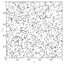
These more or less fundamental, physical sources of randomness are not behind functions like rand(), however. The randomness used in simulations is generated mathematically, not physically. And this is where the term “pseudo” comes from. Contrary to the impression you might have gotten in high school, mathematical procedures are deterministic, not random. So why do people not use physical noise in simulations?

One reason is speed: accessing an external device and postprocessing the noisy signal is much slower than having the CPU perform a few simple calculations. Another reason is reproducibility. With physical noise, each run of a simulation yields a different result. But a numerical experiment like a simulation should be reproducible. You might object that real, physical experiments are always subject to uncontrollable noise. That’s right, but the experimentalists work hard to reduce this noise as much as possible. And the advantage of numerical experiments is that we can control everything, including the noise. And we don’t want to give up this position. And, of course, reproducibility is mandatory when it comes to debugging.

So how does a purely mathematical random number generator work? The main idea is to generate a sequence $(r)=r_{1},r_{2},\ldots$ of pseudo-random numbers by a recurrence

$$r_{i}=f(r_{i-1},r_{i-2},\ldots,r_{i-n})\,,$$ (1)

and the art of random number generation lies in the design of the function $f$. Note that we need to provide the first $n$ numbers to get this recurrence off the ground. This is called seeding, and your favourite programming language has a command for this, like srand(seed) in C. Since (1) is deterministic, the only randomness involved is the choice of the seed, which is then “spread out” over a whole, usually very long sequence of numbers. It is quite surprising that this bold approach actually works!

2.1 Linear Recurrences and Randomness

We can mimic true randomness by pseudo randomness well enough, provided our recurrence is properly designed. One method to generate pseudo random integers between $0$ and some prime number $p$ is the linear recurrence

$$r_{i}=a_{1}r_{i-1}+a_{2}r_{i-2}+\ldots+a_{n}r_{i-n}\bmod p\,.$$ (2)

Here it is the $\bmod$ operation that introduces some randomness by mimicking the circular arrangement of a roulette wheel. The quality of this method depends on the magic numbers $a_{1},\ldots,a_{k}$, and to some extent on $n$ and $p$. Sequences generated by (2) are called linear feedback shift register sequences, or LFSR sequences for short.

Figure 2: Sequences generated by $x_{k}=x_{k-1}+4x_{k-2}\bmod 5$ (left) and $x_{k}=x_{k-1}+3x_{k-2}\bmod 5$ (right).

Obviously, any sequence generated by (2) is periodic. As a basic requirement we want the period of the sequence to be as large as possible. The tuple $(r_{i-1},\ldots,r_{i-n})$ can take on $p^{n}$ different values, and the all zero tuple is a fixed point. Hence the maximum period of the sequence is

$$T=p^{n}-1\,.$$ (3)

Can we choose the coefficients $a_{i}$ such that the period takes on the maximum value?

As a toy example consider the LFSR sequence

$$x_{k}=x_{k-2}+4x_{k-1}\bmod 5\,.$$

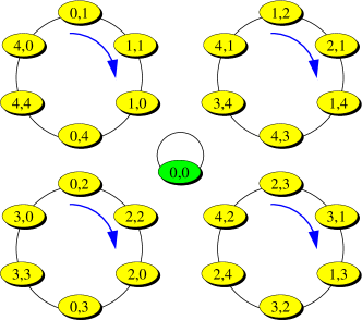
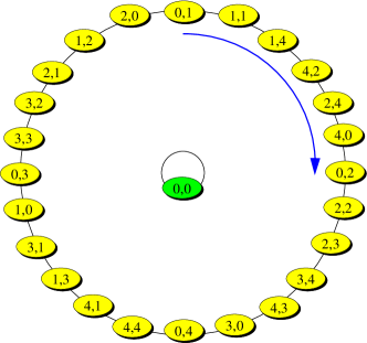
The configuration space of this recurrence is composed of $4$ sequences of period $T=6$ each, and the fixed point $(0,0)$ (Figure 2). The slightly modified recurrence

$$x_{k}=x_{k-2}+3x_{k-1}\bmod 5$$

achieves the maximum period $T=5^{2}-1$ and traces the whole configuration space except $(0,0)$ (Figure 2).

The theory behind this requires some bits of the mathematics of finite fields. Remember that the set of integers $\{0,\ldots,p-1\}$ together with addition and multiplication modulo $p$ form a finite field $\mathbb{F}_{p}$ if $p$ is prime. The corresponding theorem is this:

Theorem 2.1

The LFSR sequence (2) has maximum period $p^{n}-1$ if and only if the characteristic polynomial

$$f(x)=x^{n}-a_{1}x^{n-1}-a_{2}x^{n-2}-\ldots-a_{n}$$ (4)

is primitive modulo $p$.

A monic polynomial $f(x)$ of degree $n$ over $\mathbb{F}_{p}$ is primitive modulo $p$, if it is irreducible (i.e., cannot be factorized over $\mathbb{F}_{p}$), and if it has a primitive element of the extension field $\mathbb{F}_{p^{n}}$ as one of its roots. An element $\alpha$ of a field $\mathbb{F}$ is primitive if the powers of $\alpha$ generate $\mathbb{F}\setminus 0$. Primitive polynomials are not hard to find, and there are plenty of them for given values of $p$ and $n$.

In our toy example above, $f(x)=x^{2}-x-4$ is irreducible, but not primitive. Let $\alpha$ be a root of $f$, i.e., $\alpha^{2}=\alpha+4$. Then

$\alpha^{1}=\alpha$	$\alpha^{2}=4+\alpha$	$\alpha^{3}=4$
$\alpha^{4}=4\alpha$	$\alpha^{5}=1+4\alpha$	$\alpha^{6}=1$

hence $\alpha$ does generate only 6 of the 24 elements of $\mathbb{F}_{5^{2}}\setminus 0$. Here the order of $\alpha$ equals the period of the LFSR sequence, and this is true in general.

The roots of the irreducible $f(x)=x^{2}-x-3$ are primitive (exercise), hence the corresponding LFSR sequence has maximum period.

The following two theorems tell us that LFSR sequences with maximum period share some features with sequences of truly random numbers.

Theorem 2.2

Let $(r)$ be a LFSR sequence (2) with period $T=p^{n}-1$. Then each $k$-tuple $(r_{i+1},\ldots,r_{i+k})\in\{0,1,\ldots,p-1\}^{k}$ occurs $p^{n-k}$ times per period for $k\leq n$, except the all zero tuple for $k=n$, which never occurs.

If a tuple of $k$ successive terms $k\leq n$ is drawn from a random position of $(r)$, the outcome is uniformly distributed over all possible $k$-tuples in $\mathbb{F}_{p}$. This is exactly what one would expect from a truly random sequence.

Theorem 2.3

Let $(r)$ be a LFSR sequence (2) with period $T=p^{n}-1$ and let $\alpha$ be a complex $p$th root of unity and $\overline{\alpha}$ its complex conjugate. Then

$$C(h):=\sum_{i=1}^{T}\alpha^{r_{i}}\cdot\overline{\alpha}^{r_{i+h}}=\begin{cases}T&\text{if $h=0\bmod T$}\\ -1&\text{if $h\neq 0\bmod T$}\end{cases}\,.$$ (5)

$C(h)$ can be interpreted as the autocorrelation function of the sequence, and Theorem 2.3 tells us that LFSR sequences with maximum period have a flat autocorrelation function. Again this is a property (white noise) that is also observed in truly random sequences.

Theorems 2.2 and 2.3 are the reason why LFSR sequences with maximum period are called pseudonoise sequences. As you can guess by now, they are excellent recipes for PRNGs.

2.2 Yet Another Random Number Generator

If you check the internet or consult textbooks on random number generation, you will usually find all sorts of nonlinear generators. The rationale for going nonlinear is that linear recurrences have some known weaknesses. Another motivation is the belief that more complicated rules generate more random output. If you agree with the latter statement, have a look at [9], in which Donald Knuth tells the story how he designed a tremendously involved algorithm which one can’t even write down as a simple recurrence. His goal was to create an “extremely random” PRNG, but to his surprise, his rule runs into a fixed point after just a few iterations. It was completely useless as a PRNG. The moral of this story:

Random number generators should not be chosen at random.

Some theory should be used. Unfortunately, the theory of nonlinear recurrences is much less developed than the theory of linear recurrences. So let’s stick for the moment with linear pseudonoise sequences and have a look at their weaknesses.

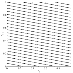
The points in the middle of Figure 1 have been generated by taking two consecutive and properly scaled values of the linear recurrence

$$r_{i+1}=95r_{i}\bmod 1999$$ (6)

as coordinates. This is a pseudonoise sequence, but it doesn’t look random at all, at least not in this experiment. The linear structure that survives the $\bmod$-operation is clearly visible. We can get rid of this effect by using a linear recurrence with more feedback taps, i.e., with $n>1$. But the linear structure reappears when we sample points in $d$ dimensional space with $d>n$.

Theorem 2.2 tells us that pseudonoise sequences, when used to sample coordinates in $d$-dimensional space, cover every point for $d<n$, and every point except $(0,0,\ldots,0)$ for $d=n$. For $d>n$ the set of positions generated is obviously sparse, and the linearity of the rule (2) leads to the concentration of the sampling points on $n$-dimensional hyperplanes. This phenomenon, first noticed by Marsaglia in 1968 [10], motivates one of the well known empirical tests for PRNGs, the so-called spectral test [9]. The spectral test checks the behavior of a generator when its outputs are used to form $d$-tuples. Linear sequences can fail the spectral test in dimensions larger than the register size $n$. Closely related to this mechanism are the observed correlations in other empirical tests like the birthday spacings test and the collision test. Nonlinear generators do quite well in all these tests, but compared to linear sequences they have much less nice and provable properties. And they cannot be properly parallelized, as we will see below.

To get the best of both worlds we can use a delinearization that preserves all the nice properties of linear pseudonoise sequences:

Theorem 2.4

Let $(q)$ be a linear pseudonoise sequence in $\mathbb{F}_{p}$, and let $g$ be a generating element of the multiplicative group $\mathbb{F}^{*}_{p}$. Then the sequence $(r)$ with

$$r_{i}=\begin{cases}g^{q_{i}}\bmod p&\text{if $q_{i}>0$}\\ 0&\text{if $q_{i}=0$}\end{cases}$$ (7)

is a pseudonoise sequence, too.

The proof of this theorem is trivial: since $g$ is a generator of $\mathbb{F}^{*}_{p}$, the map (7) is bijective. We call a generator based on (7) YARN generator (yet another random number).

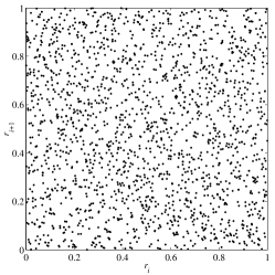
The exponentiation largely destroys the linear structure. This can be seen in the rightmost plot in Figure 1, which has been generated by

$$q_{i} =95q_{i-1}\bmod 1999$$

$$r_{i} =1099^{q_{i}}\bmod 1999\,.$$

Visually, this delinearized sequence scatters the points much more randomly than the underlying linear version. In fact, YARN type generators pass the corresponding empirical tests (spectral tests, coupon collector, etc.) with flying colors, but there is an even more convincing argument that exponentiation removes all traces of linearity. This argument is based on the following theorem:

Theorem 2.5

All finite length sequences and all periodic sequences over a finite field $\mathbb{F}_{p}$ can be generated by a linear recurrence (2).

This theorem implies that any recurrent sequence of integer numbers of a finite domain, i.e., every sequence that a computer program can generate, is equivalent to some linear recurrence in $\mathbb{F}_{p}$. In this sense, pseudorandomness is always linear.

Prima facie, Theorem 2.5 is counterintuitive. But note that it says nothing about order of the linear recurrence. The linear complexity of a sequence is the minimum order of a linear recurrence that generates this sequence. Consider the hardest case: a sequence of $\ell$ truly random numbers between $0$ and $p-1$. A truly random sequence of $\ell$ numbers cannot be compressed, i.e., expressed by less than $\ell$ numbers. Hence we expect the linear complexity of $\ell$ random numbers to be $\ell/2$: half of the information is contained in the coefficients, the other half in in the seed. In fact one can prove that the average linear complexity of an $\ell$ element random sequence is $\ell/2$.

Typically the linear complexity of a nonlinear sequence is of the same order of magnitude as the period of the sequence. Since the designers of PRNGs strive for “astronomically” large periods, implementing nonlinear generators as a linear recurrences is not tractable. As a matter of principle, however, any nonlinear recurrence can be seen as an efficient implementation of a large order linear recurrence. The popular “Mersenne Twister” [11] for example is an efficient nonlinear implementation of a linear recurrence in $\mathbb{F}_{2}$ of order 19 937.

The coefficients and the initial seed of the minimum order linear recurrence can be calculated very efficiently, i.e., polynomially in the minimum order, using the Berlekamp-Massey algorithm [8].

Figure 3: Linear complexity profile $L_{(r)}(l)$ of a YARN sequence, produced by the recurrence $q_{i}=173\cdot q_{i-1}+219\cdot q_{i-2}\bmod 317$ and $r_{i}=151^{q_{i}}\bmod 317$. The period of this sequence is $T=317^{2}-1$.

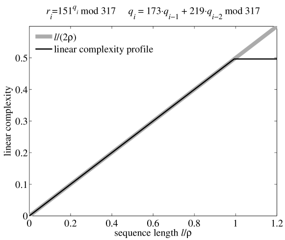
If we feed a stream of numbers from a PRNG to the Berlekamp-Massey algorithm, we get its linear complexity as a function of the length $\ell$ of the stream. For a LFSR sequence (2), this linear complexity profile quickly reaches a plateau at $\ell=n$, whereas for a truly random stream we expect the profile to grow like $\ell/2$. Figure 3 shows that the linear complexity of a YARN generator does grow like $\ell/2$ for $\ell\leq T/2$. Measured in terms of linear complexity, YARN generators are as random and nonlinear as it can get.

3 Parallelization

In parallel applications we need to generate streams $t_{j,i}$ of random numbers, where $j=0,1,\dots,p-1$ numbers the streams for each of the $p$ processes. We require statistical independency of the $t_{j,i}$ within each stream and between the streams.

Since random numbers are very often needed in the innermost loop of a simulation, efficiency of a PRNG is very important. We require that a PRNG can be parallelized without loosing its efficiency.

And there is a third requirement besides quality and speed: we want the simulation to play fair. We say that a parallel Monte Carlo simulation plays fair, if its outcome is strictly independent of the underlying hardware, where strictly means deterministically, not just statistically. Fair play implies the use of the same pseudo random numbers in the same context, independently of the number of parallel processes. It is mandatory for debugging, especially in parallel environments where the number of parallel processes varies from run to run, but another benefit of playing fair is even more important: Fair play guarantees that the quality of a PRNG with respect to an application does not depend on the degree of parallelization. In this sense, fair play conserves quality.

It is not always easy to implement a Monte Carlo simulation such that it plays fair. For some Monte Carlo algorithms it may even be impossible. But for many simulation algorithms it is possible—provided the underlying PRNG supports fair parallelization. We will see that some straightforward parallelization techniques for PRNGs prevent fair play even in the simplest simulation, while others support fair play in moderately complicated situations.

3.1 Random Seeding and Parameterization

One parallelization technique is random seeding: All processes use the same PRNG but a different “random” seed. The hope is that they will generate non-overlapping and uncorrelated subsequences of the original PRNG. This hope, however, has little theoretical foundation. Random seeding is a clear violation of Don Knuth’s advice cited above. Yet this approach is frequently used in practice because it works with any PRNG, is easy to program and comes without any penalty on the efficiency. With random seeding, however, no simulation can play fair.

Another parallelization technique is parameterization: All processes use the same type of generator but with different parameters for each processor. Example: linear congruential generators with additive constant $b_{j}$ for the $j$th stream

$$t_{j,i}=a\cdot t_{j,i-1}+b_{j}\bmod m\,,$$ (8)

where the $b_{j}$’s are different prime numbers just below $\sqrt{m/2}$. Another variant uses different multipliers $a$ for different streams. The theoretical foundation of these methods is weak, and empirical tests have revealed serious correlations between streams. On massive parallel system you may need thousands of parallel streams, and it is not trivial to find a type of PRNG with thousands of “well tested” parameter sets.

Like random seeding, parameterization prevents fair play. Therefore both methods should be avoided.

3.2 Block Splitting and Leapfrogging

Block splitting is the idea to break up a single stream of random numbers into non-overlapping, consecutive blocks of numbers and assign each block to one of the processes.

Let $M$ be the maximum number of calls to a PRNG by each processor, and let $p$ be the number of processes. Then we can split the sequence $(r)$ of a sequential PRNG into consecutive blocks of length $M$ such that

$$\begin{split}t_{0,i}&=r_{i}\\ t_{1,i}&=r_{i+M}\\ &\dots\\ t_{p-1,i}&=r_{i+M(p-1)}\,.\end{split}$$ (9)

This method works only if we know $M$ in advance or can at least safely estimate an upper bound for $M$. For an efficient block splitting, it is necessary to jump from the $i$th random number to the $(i+M)$th number without calculating the numbers in between. Block splitting is illustrated in Figure 4.

The leapfrog method distributes a sequence $(r)$ of random numbers over $d$ processes by decimating this base sequence such that

$$\begin{split}t_{0,i}&=r_{di}\\ t_{1,i}&=r_{di+1}\\ &\dots\\ t_{d-1,i}&=r_{di+(d-1)}\,.\end{split}$$ (10)

Leapfrogging is illustrated in Figure 4. It does not require an a priori estimate of how many random numbers will be consumed by each processor.

Figure 4: Parallelization by block splitting (left) and leapfrogging (right).

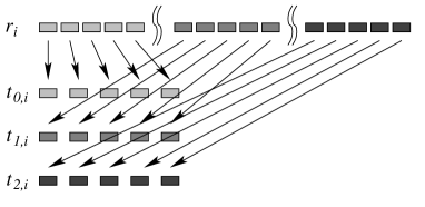
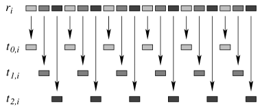
Note that for a periodic sequence $(r)$ the substreams derived from block-splitting are cyclic shifts of the original sequence $(r)$, and for $p$ not dividing the period of $(r)$, the leapfrog sequences are cyclic shifts of each other. Hence the leapfrog method is equivalent to block-splitting on a different base sequence.

Leapfrog and block splitting support fair play, i.e., they allow us to program parallel simulations that use the same random numbers in the same context idependently of the number of parallel streams.

As an illustrative example we consider the site percolation problem. A site in a lattice of size $N$ is occupied with some probability, and the occupancy is determined by a pseudo random number. $M$ random configurations are generated.

A fair playing percolation simulation can be organized by leapfrogging on the level of lattice configurations. Here each process consumes distinct contiguous blocks of numbers from the sequence $(r)$, and the workload is spread over $d$ processors in such a way that each process analyses each $d$th lattice. If we number the processes by their rank $i$ from $0$ to $d-1$ and the lattices from $0$ to $M-1$, each process starts with a lattice whose number equals its own rank. That means process $i$ has to skip $i\cdot N$ random numbers before the first lattice configuration is generated. Thereafter each process can skip $d-1$ lattices, i. e., $(d-1)\cdot N$ random numbers, and continue with the next lattice.

Organizing simulation algorithms such that they play fair is not always as easy as in the above example, but with a little effort one can achieve fair play in more complicated situations, too. This may require the combination of block splitting and the leapfrog method, or iterated leapfrogging. Sometimes it is also necessary to use more than one stream of random numbers per process, as we will see below.

3.3 Parallelization of Linear Recurrences

We can “simulate” block splitting and leapfrogging by throwing away all random numbers that are not from the right block or from the right leapfrog subsequence. This works for any PRNG, but it is not very efficient and foils parallelization. For an efficient parallelization, we should be able to modify a PRNG to generate directly only every $d$th element of the original sequence (for leapfrogging) or to directly advance the PRNG by $M$ steps (for block splitting). For LFSR sequences (2), both can be achieved very efficiently.

Let’s start with block splitting, i.e., with jumping ahead in a linear recurrence. Note that by introducing a companion matrix $A$ the linear recurrence (2) can be written as a vector matrix product:

$$\begin{pmatrix}r_{i-(n-1)}\\ \vdots\\ r_{i-1}\\ r_{i}\end{pmatrix}=\underbrace{\begin{pmatrix}0&1&\dots&0\\ \vdots&\vdots&\ddots&\vdots\\ 0&0&\dots&1\\ a_{n}&a_{n-1}&\dots&a_{1}\end{pmatrix}}_{\displaystyle A}\begin{pmatrix}r_{i-n}\\ \vdots\\ r_{i-2}\\ r_{i-1}\end{pmatrix}\bmod p$$ (11)

From this formula it follows immediately that the $M$-fold successive iteration of (2) may be written as

$$\begin{pmatrix}r_{i-(n-1)}\\ \vdots\\ r_{i-1}\\ r_{i}\end{pmatrix}=A^{M}\begin{pmatrix}r_{i-M-(n-1)}\\ \vdots\\ r_{i-M-1}\\ r_{i-M}\end{pmatrix}\bmod p\,.$$ (12)

Matrix exponentiation can be accomplished in $\mathcal{O}\left(n^{3}\ln M\right)$ steps via binary exponentiation, also known as exponentiation by squaring.

Implementing leapfrogging efficiently is less straightforward. Calculating $t_{j,i}=r_{di+j}$ via

$$\begin{pmatrix}r_{di+j-(n-1)}\\ \vdots\\ r_{di+j-1}\\ r_{di+j}\end{pmatrix}=A^{d}\begin{pmatrix}r_{d(i-1)+j-(n-1)}\\ \vdots\\ r_{d(i-1)+j-1}\\ r_{d(i-1)+j}\end{pmatrix}\bmod m$$ (13)

is no option, because $A^{d}$ is usually a dense matrix, in which case calculating a new element from the leapfrog sequence requires $\mathcal{O}(n^{2})$ operations instead of $\mathcal{O}(n)$ operations as in the base sequence.

Obviously the linear complexity of a leapfrog subsequence cannot be larger than the linear complexity of the underlying base sequence, which for LFSR sequences is $n$. Hence all we need to do is to generate at most $2n$ elements of the leapfrog sequence and feed them to the Berlekamp-Massey algorithm. This yields the coefficients and the seed for an LFSR generator that produces the leapfrog subsequence. This is how leapfrogging for LFSR sequences is done in practice.

Note that the techniques for block splitting and for leapfrogging of LFSR sequences also work for YARN generators by simply applying them to the underling LFSR sequence.

4 From Theory to Practice: TRNG

We will illustrate the use of pseudo random generators in parallel simulations by means of TRNG, a C++ library for sequential and parallel Monte-Carlo simulations. TRNG has several outstanding features that set it apart from other random number libraries:

1. Its current version (4.7) contains a collection of different PRNGs, like various LFSR and YARN generators, lagged Fibonacci sequences, 32-bit and 64-bit implementations of the Mersenne-Twister, etc.

2. Its C++ interface makes it very easy to switch PRNGs in your simulation, even if your program is completely written in C (see below).

3. Parallelization by leapfrogging and block-splitting is fully supported for all generators that can be parallelized.

4. The internal state of each PRNG can be written to and read from a file. This allows us to stop a simulation and carry on later, which is especially useful for long running simulations that face the risk of hardware failure or system maintenance before they are done.

5. TRNG implements a large variety of distributions, from standard distributions like uniform, exponential or Poisson distributions to lesser known distributions like Fisher-Snedecor- and Rayleigh-distributions. Each distribution comes with functions to calculate its probability density, its cumulative distribution and, in the case of continuous distributions, its inverse cumulative distribution.

6. The interface of TRNG complies to the ISO C++ standard for PRNGs [3] and to the random number generator interface defined in the Standard Template Library (STL) for C++ [7].

7. Last but not least: TRNG is free. You can get the source code and the documentation from trng.berlios.de.

4.1 Basics

TRNG is a set of classes of two types: random number engines (the actual PRNGs) and probability distributions. Each class is defined in its own header file. Lets suppose that we want to use random number generators of the YARN type (for the parallel part) and a Mersenne twister generator for the sequential part. We will generate uniform variates from the interval $[0,1)$ and Poisson variates. The corresponding header files read

   #include <trng/yarn2.hpp>
   #include <trng/mt19937.hpp>
   #include <trng/uniform01_dist.hpp>
   #include <trng/poisson_dist.hpp>

and the PRNGs and distributions are declared as

   trng::yarn2 rand1, rand2;  // two generators of type YARN
   trng::mt19937 rand3;       // Mersenne twister
   trng::uniform01_dist<double> uniform;
   trng::poisson_dist poisson(2.0);  // mean value is 2.0

Note that we specified the uniform distribution to return numbers of type double. Alternatively we could have specified float or long double. The Poisson distribution returns integer values, of course.

The ’2’ in the classname yarn2 denotes the order of the underlying LFSR. The feedback parameters are set to well chosen default values, but TRNG allows users to supply their own paremeters.

The use of the generators is very simple:

   k = poisson(rand3);  // use Mersenne twister to generate Poisson variate
   ...
   if (uniform(rand1) < 0.5) {
     // do this with probability one half
     ...
   }

Most of the random number engines in TRNG are parallelizable, i.e., they have member functions for leapfrogging and block-splitting. Let nprocs denote the total number of parallel processes, and let rank denote the ordinal number of the current process. A parallel simulation code typically contains lines like

  rand1.split(nprocs,rank);

This line modifies the random number engine rand1 such that it generates leapfrog substream rank out of nprocs total substreams.

For block-splitting there exist two functions:

  rand1.jump(M); // advance by M steps
  rand2.jump1(n); // advance by 2^n steps

4.2 Example: Broken Triangles

To see how TRNG is used in a concrete situation, let’s develop a parallel Monte Carlo code to analyse the following problem:

If two points are independently and uniformly located in the unit interval, they divide that interval into three segments. What is the probability that those three segments form a triangle? And what is the probability that the triangle is obtuse?

The mathematical background of this problem is very simple: Line segments of lengths $a$, $b$ and $c$ can be arranged as a triangle if and only if all lengths obey the triangle inequality, i.e., if and only if

$$a\leq b+c\qquad b\leq a+c\qquad c\leq a+b\,.$$ (14)

We recall from high school geometry that the interior angles of a triangle $\alpha$, $\beta$ and $\gamma$ are given by

$$\cos\alpha=\frac{b^{2}+c^{2}-a^{2}}{2bc},\qquad\cos\beta=\frac{a^{2}+c^{2}-b^{2}}{2ac},\qquad\cos\gamma=\frac{a^{2}+b^{2}-c^{2}}{2ab}\,.$$ (15)

A triangle is obtuse if one of the angles is larger than $90$, i.e., if one of the nominators is negative.

In our Monte Carlo algorithm for the triangle problem, we generate two random numbers $r_{1}$ and $r_{2}$ uniformly and independently from the unit interval and calculate the lengths of the segments

$$a=\min(r_{1},r_{2})\qquad b=\max(r_{1},r_{2})-\min(r_{1},r_{2})\qquad c=1-\max(r_{1},r_{2})\,.$$

Then we check (14) and the nominators of (15) to see whether the segments form an (obtuse) triangle. We repeat this experiment over and over again and count the fraction of (obtuse) triangles.

Once again we assume that the number of running processes and the rank of a process are stored in the variables nprocs and rank. The core part of our parallel simulation then reads

  trng::yarn2 r1, r2;

  r1.seed (seed);

  // first splitting yields two random sources for the two cuts
  r2 = r1;
  r1.split (2,0); r2.split (2,1); // ...

  // second splitting for parallelization
  r1.split (nprocs,rank); r2.split (nprocs,rank);

  // main loop
  triangles = 0; obtuse = 0;
  for (k = 0; k < MCS; k += nprocs) { // MCS: number of total samples
    a = uniform(r1);
    b = uniform(r2);
    if (a > b) {c = a; a = b; b = c;} // ensure a <= b
    c = 1.0 - b;
    b = b-a;
    if ((a+b >= c) && (a+c >= b) && (b+c >= a)) {
      triangles++;
      if ((a*a+b*b < c*c) || (a*a+c*c < b*b) || (b*b+c*c < a*a)) obtuse++;
    }
  }

We used leapfrogging twice. The first split creates two sequences, one for each random cut into the unit interval. Then both sequences are split according to the number of parallel processes. The loop is written such that each process gets the same workload.

The complete program has additional code for getting the values for nprocs and rank, for distributing the seed among all processes and for collecting the results from all processes. Since this part depends on the parallel machinery (like MPI or OpenMP), we will not discuss it here. But you are encouraged to complete the program and run it.

Here is the output of a MPI implementation running on 20 processes, with seed $141164$ and using $10000$ samples:

  /home/mertens> mpirun -np 20 mpi_triangle -S 141164 -M 10000
  # number of processes: 20
  # PRNG: yarn2 from TRNG 4.7
  # seed    = 141164
  # samples = 10000
  # fraction of triangles: 0.2481
  # fraction of obtuse triangles: 0.1725

This result is within the error bars of the exact values

$$p(\text{triangle})=\frac{1}{4}\qquad p(\text{obtuse triangle})=\frac{9}{4}-3\ln 2=0.170558\ldots\,,$$

hence we are confident that our program is correct. But if we run it with exactly the same parameters on 30 processes, we get

  /home/mertens> mpirun -np 30 mpi_triangle -S 141164 -M 10000
  # number of processes: 30
  # PRNG: yarn2 from TRNG 4.7
  # seed    = 141164
  # samples = 10000
  # fraction of triangles: 0.2486
  # fraction of obtuse triangles: 0.1728

The deviation from the previous run is small and well within the statistical error. But wait! We are running a fair simulation. The output must not depend on the number of parallel processes. The tiny deviation tells us that our program is not correct. Try to find the bug in the code above!

4.3 Final Remarks

“Which random number generator is the best? Which one shall I use in my simulations?” These questions are inevitably asked after each and every talk on PRNGs. The answer is simple: There is no such thing as the “best” generator. Most generators are advertised with a phrase like “this generator has passed a battery of statistical tests”. But a generator that has passed $N-1$ statistical tests may fail the $N$th test—your simulation. And LFSR sequences that fail the spectral test, work perfectly in most applications that do not sample points in high dimensional space. The rule is, that your simulation should not be sensitive to the inevitable correlations in a PRNG [1]. But how can we know? By following rule number one:

Rule I:

Run your simulation at least twice, each time with a different type of PRNG.

If the results of all runs agree within the statistical error, we are on the safe side.

In order to enable others to repeat your numerical experiments, the type of PRNG must be published along with the results. In addition, the PRNG and the seed used in the run should be stored with the data:

Rule II:

The type of PRNG that has been used must be published along with the results. The seed must be stored in the original data files.

Quite often, Monte Carlo simulations screw up not because of a bad PRNG but because of the bad usage of a PRNG. The classical example is to (mis)use a $32$-bit random integer to sample a list of $2^{36}$ elements. Such a list corresponds to $64$ GBytes, which is not an uncommon size. This brings us to

Rule III:

Know your PRNG, especially its limitations (numerical resolution, period length, statistical quality of low order bits, etc.).

Last but not least:

Rule IV:

Parallel simulations should be programmed to play fair, and fair play should explicitely be checked.

5 Further Reading

This lecture is mainly based on the paper that introduces the YARN generator and the concept of fair play in Monte-Carlo simulations [2]. The references in this paper can be used as a starting point for a journey into the wondrous world of pseudo randomness. Another good starting point is Brian Hayes’ nice essay “Randomness as a Resource” [6].

If you want to learn more about the theory behind pseudo random number generators, Donald Knuth’s classical tome [9] is the right choice. An excellent introduction to finite fields is Jungnickel [8].

Every physicist who is using random number generators should know about the Ferrenberg affair: In 1992, Alan Ferrenberg, David Landau and Joanna Wong discovered that a family of established random number generators yield wrong results in Monte Carlo simulations of the Ising model [4]. This was a shock to the community because up to this moment, everybody trusted PRNGs that had passed the infamous “battery of statistical tests”. Read Brian Hayes’ depiction of the Ferrenberg affair and its aftermath [5]. The forensic analysis of the affair is also recommended reading [12].

If you want to see how (and why) well established PRNGs fail dramatically even in very simple simulations, you will enjoy [1].

Bibliography

- [1] Heiko Bauke and Stephan Mertens. Pseudo random coins show more heads than tails. J. Stat. Phys., 114:1149–1169, 2004.
- [2] Heiko Bauke and Stephan Mertens. Random numbers for large scale distributed Monte Carlo simulations. Phys. Rev. E, 75:066701, 2007.
- [3] Walter E. Brown, Mark Fischler, Jim Kowalkowski, and Marc Paterno. Random Number Generation in C++0X: A Comprehensive Proposal, version 2, 2006. http://www.open-std.org/jtc1/sc22/wg21/docs/papers/2006/n2032.pdf.
- [4] Alan M. Ferrenberg and David P. Landau and Y. Joanna Wong. Monte carlo simulations: Hidden errors from “good” random number generators. Physical Review Letters, 69(23):3382–3384, 1992.
- [5] Brian Hayes. The wheel of fortune. American Scientist, 81(2):114–118, March/April 1993.
- [6] Brian Hayes. Randomness as a resource. American Scientist, 89(4):300–304, July/August 2001.
- [7] Nicolai Josuttis. The C++ Standard Library. Addison Wesley, Boston, 1999.
- [8] Dieter Jungnickel. Finite Fields: Structure and Arithmetics. Bibliographisches Institut, 1993.
- [9] Donald E. Knuth. The Art of Computer Programming, volume 2: Seminumerical Algorithms. Addison Wesley Professional, 3rd edition, 1998.
- [10] George Marsaglia. Random numbers fall mainly in the planes. Proceedings of the National Academy of Sciences, 61:25–28, 1968.
- [11] Makoto Matsumoto and Takuji Nishimura. Mersenne twister: A 623-dimensionally equidistributed uniform pseudo-random number generator. ACM Transactions on Modeling and Computer Simulation, 8(1):3–30, 1998.
- [12] Stephan Mertens and Heiko Bauke. Entropy of pseudo random number generators. Phys. Rev. E, 69:055702(R), 2004.