Security Analysis of an Untrusted Source for Quantum Key Distribution: Passive Approach

Abstract

We present a passive approach to the security analysis of quantum key distribution (QKD) with an untrusted source. A complete proof of its unconditional security is also presented. This scheme has significant advantages in real-life implementations as it does not require fast optical switching or a quantum random number generator. The essential idea is to use a beam splitter to split each input pulse. We show that we can characterize the source using a cross-estimate technique without active routing of each pulse. We have derived analytical expressions for the passive estimation scheme. Moreover, using simulations, we have considered four real-life imperfections: Additional loss introduced by the “plug & play” structure, inefficiency of the intensity monitor, noise of the intensity monitor, and statistical fluctuation introduced by finite data size. Our simulation results show that the passive estimate of an untrusted source remains useful in practice, despite these four imperfections. Also, we have performed preliminary experiments, confirming the utility of our proposal in real-life applications. Our proposal makes it possible to implement the “plug & play” QKD with the security guaranteed, while keeping the implementation practical.

1 Introduction

Quantum key distribution (QKD) provides a means of sharing a secret key between two parties, a sender Alice and a receiver Bob, securely in the presence of an eavesdropper, Eve [1, 2, 3]. The unconditional security of QKD has been rigorously proved [4], even when implemented with imperfect real-life devices [5, 6]. Decoy state method was proposed [7, 8, 9, 10, 11, 12] and experimentally demonstrated [13, 14] as a means to dramatically improve the performance of QKD with imperfect real-life devices with unconditional security still guaranteed [5, 9].

A large class of QKD setups adopts the so-called “plug & play” architecture [15, 16]. In this setup, Bob sends strong pulses to Alice, who encodes her quantum information on them and attenuates these pulses to quantum level before sending them back to Bob. Both phase and polarization drifts are intrinsically compensated, resulting in a very stable and relatively low quantum bit error rate (QBER). These significant practical advantages make the “plug & play” very attractive. Indeed, most current commercial QKD systems are based on this particular scheme [17, 18].

The security of “plug & play” QKD was a long-standing open question. A major concern arises from the following fact: When Bob sends strong classical pulses to Alice, Eve can freely manipulate these pulses, or even replace them with her own sophisticatedly prepared pulses. That is, the source is equivalently controlled by Eve in the “plug & play” architecture. In particular, it is no longer correct to assume that the photon number distribution is Poissonian, as is commonly assumed in standard security proof. This is a major reason why standard security proofs such as GLLP [5] does not appear to apply directly to the “plug and play” scheme.

It might be tempting to apply the central limit theorem [19] to the current problem. That is, the photons contained in a pulse after heavy attenuation obeys a Gaussian distribution asymptotically. The central limit theorem was adopted in [20].

However, the central limit theorem does not apply to the situation that the current paper is addressing. The current paper, as well as a previous work [21], does not rely on the central limit theorem and removes the assumption on the input photon number distribution. i.e., our analysis applies to sources with an arbitrary photon number distribution. For example, imagine a source that follows a dual-delta distribution (i.e., the pulses sent by the source contain either $n_{1}$ or $n_{2}$ photons, where $n_{1}$ and $n_{2}$ are large and different integers). In this case, even if Alice applies heavy attenuation on the input pulses, the resulting photon number per pulse distribution would be the sum of two Gaussian distributions, which in general is not a Gaussian distribution.

The dual-delta distributed source is of significant practical meaning rather than a purely imaginary source. Consider the case of the Trojan horse attack [20]: An eavesdropper occasionally sends bright pulse to Alice and splits the corresponding output signal from Alice. In this case, the input photon number per pulse distribution on Alice’s side would have two peaks: one corresponds to the photon number of the authentic source, and one corresponds to the sum of the photon numbers from the two pulses (one from the authentic source and the other one from the eavesdropper’s probing pulse). The security analysis that is based on the central-limit theorem (e.g., Ref. [20]) may not be directly applicable to this case. However, the analysis proposed in [21] and in the current paper can analyze such case simply by defining an appropriate input photon number range of the untagged bits such that most input pulses are included. Note that, the input photon number range for the untagged bits is defined in the post-processing stage, during which Alice has already collected the photon number distribution of the samples.

Figure 1: A general schematic of secure QKD with unknown and untrusted source. The Filter guarantees the single mode assumption. The Phase Randomizer guarantees the phase randomization assumption. The Photon Number Analyzer (PNA) estimates photon number distribution of the source. Various PNAs are shown in Figure 2.

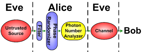
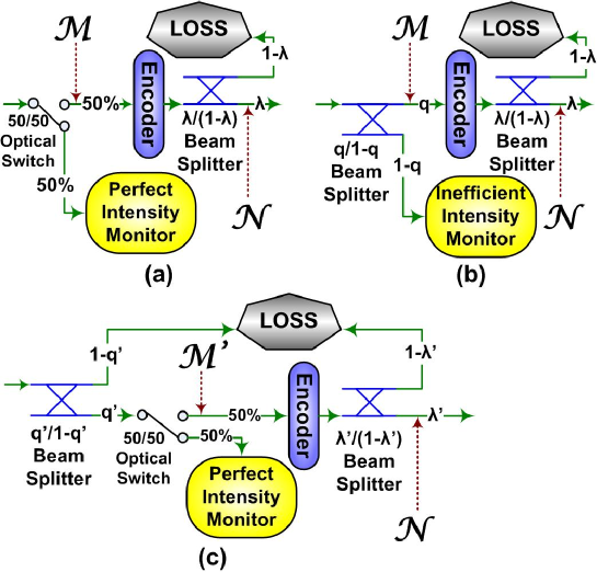
The unconditional security of “plug & play” QKD scheme has been recently proven in [21]. The basic idea is illustrated in Figure 1. A Filter guarantees the single mode assumption. A Phase Randomizer guarantees the phase randomization assumption. Note that for the state that is accessible to the eavesdropper, Alice’s phase randomization is equivalent to a quantum non-demolition (QND) measurement of the photon numbers of the optical pulses. See A for details. Therefore, from now on, without loss of generality, we will assume that Alice’s input signal is a classical mixture of Fock states and, similarly Alice’s output signal is also a classical mixture of Fock states. A Photon Number Analyzer (PNA) estimates photon number distribution of the source. Detail of the PNA in [21] is shown in Figure 2(a).

Figure 2: Different schemes to estimate photon number distribution. $\mathcal{M}$, $\mathcal{M^{\prime}}$, and $\mathcal{N}$ are random variables for input photon number, virtual input photon number, and output photon number, respectively. All the internal loss of Alice is modeled as a $\lambda/1-\lambda$ beam splitter (in (a) and (b)) or a $\lambda^{\prime}/1-\lambda^{\prime}$ beam splitter (in (c)). (a) active scheme; (b) passive scheme; (c) hybrid scheme. $q^{\prime}=\eta_{\mathrm{IM}}(1-q)$, where $\eta_{\mathrm{IM}}\leq 1$ is the efficiency of the imperfect intensity monitor. $\lambda^{\prime}=q\lambda/q^{\prime}$. Note that the scheme shown in (c) is a virtual set-up that has features from both the active scheme (a) and the passive scheme (b). The purpose of introducing this virtual scheme (c) is to bridge the active scheme (a) and the passive scheme (b).

The analysis presented in [21] applies to a general class of QKD with unknown and untrusted sources besides “plug & play” QKD. For example, many QKD implementations use pulsed laser diodes as the light source. These laser diodes are turned on and off frequently to generate laser pulse sequence. However, such laser pulses are not in coherent state and the photon number per pulse does not obey Poisson distribution [21]. Moreover, the go-and-return scheme is also adopted by the recently proposed ground-satellite QKD project [22], in which the source is also equivalently unknown and untrusted.

[21] analyzes the photon number distribution of an untrusted source in the following manner: Each input pulse will be randomly routed to either an Encoder in Figure 2(a) as a coding pulse, or a Perfect Intensity Monitor in Figure 2(a) as a sampling pulse. The photon numbers of each sampling pulse are individually measured by the intensity monitor. In particular, one can obtain an estimate of the fraction of coding pulses that has a photon number $m\in[(1-\delta)M,(1+\delta)M]$ (here $\delta$ is a small positive real number, and $M$ is a large positive integer. Both $\delta$ and $M$ are chosen by Alice and Bob). These bits are defined as “untagged bits”. The details of security analysis results of [21] are presented in B. We note that some security analyses about QKD with a fluctuating source have been reported recently [23, 24, 25, 26].

It is challenging and inefficient to implement the scheme proposed in [21], which is referred to as an active scheme, for the following reasons: 1) The Optical Switch in Figure 2(a) is an active component and requires real-time control. The design and manufacture of the optical switch and its controlling system can be very challenging in high-speed QKD systems, which can operate as fast as 10 GHz [27]. 2) The random routing of optical pulses requires a high-speed sampling quantum random number generator (sampling QRNG), which does not yet exist for Gb/s systems. 3) The number of pulses sent to Bob is only a constant fraction (say half) of the number of pulses generated by the source, which means the key generation rate per pulse sent by the source is reduced by that fraction.

Naturally, the optical switch can be replaced by a beam splitter, which will passively split every input pulse, sending a portion into the intensity monitor and the rest to the encoder. This is referred to as a passive scheme. In this scheme, the sampling QRNG is not required.

A very recent work proposed some preliminary analysis on the passive estimation of an untrusted source using inverse Bernoulli transformation, and performed some experimental tests [28]. It is very encouraging to see that it is possible to prove the security of the passive estimate scheme for QKD with an untrusted source. As acknowledged by the authors of [28], the inverse Bernoulli transformation is beyond the computational power of current computers, and the required photon number resolution is beyond the capabilities of practical photo diodes. Owing to the above challenges, the experimental data reported in [28] were not analyzed by the analysis proposed in the same paper.

In this paper, we propose a passive scheme to estimate the photon number distribution of an untrusted source together with a complete proof of its unconditional security. We show that the unconditional security can still be guaranteed without routing each input optical pulse individually. Our analysis provides both an analytical method to calculate the final key rate and an explicit expression of the confidence level. Moreover, we considered the inefficiency and finite resolution of the intensity monitor, making our proposal immediately applicable. In the numerical simulation, we considered the additional loss introduced by the “plug & play” structure and the statistical fluctuation introduced by the finite data size. We also gave examples of imperfect intensity monitors in the simulation, in which a constant Gaussian noise is considered.

This paper is organized in the following way: in Section II, we will propose a modified active estimate method; in Section III, we will establish the equivalence between the modified active scheme proposed in Section II and passive estimate scheme; in Section IV, we will present a more efficient passive estimate protocol than the one proposed in Section III; in Section V, we will present the numerical simulation results of the protocol proposed in Section IV and compare the efficiencies of active and passive estimates; in Section VI, we will present a preliminary experiment based on our proposed passive estimate protocol.

2 Modified Active Estimate

In [21], it is shown that Alice can randomly pick a fixed number of input pulses as sampling pulses, and measure the number of untagged sampling bits. One can then estimate the number of untagged coding bits.

We find that we can modify the scheme proposed in [21] by drawing a non-fixed number of input pulses as samples. A passive estimate can be built on top of this modified active estimate scheme. Note that we only modified the way to estimate the number of untagged coding bits. Once the number of untagged coding bits is estimated, the security analysis proposed in [21] is still applicable to calculate the lower bound of secure key rate.

Lemma 1.

Consider that $k$ pulses are sent to Alice from an unknown and untrusted source, within which $V$ pulses are untagged. Alice randomly assigns each bit as either a sampling bit or a coding bit with equal probabilities (both are 1/2). In total, $V_{\mathrm{s}}$ sampling bits and $V_{\mathrm{c}}$ coding bits are untagged. The probability that $V_{\mathrm{c}}\leq V_{\mathrm{s}}-\epsilon k$ satisfies

$$P(V_{\mathrm{c}}\leq V_{\mathrm{s}}-\epsilon k)\leq\exp(-\frac{k\epsilon^{2}}{2})$$ (1)

where $\epsilon$ is a small positive real number chosen by Alice and Bob.

That is, Alice can conclude that $V_{\mathrm{c}}>V_{\mathrm{s}}-\epsilon k$ with confidence level

$$\tau>1-\exp(-\frac{k\epsilon^{2}}{2})$$ (2)

Proof.

See C. ∎

Note that the right hand side of Equation (1) is independent of $V$. This is important because Alice does not know the exact value of $V$, while Eve may know, and may even manipulate the value of $V$. Nonetheless, the inequality suggested in Equation (1) holds for any possible value of $V$. Therefore, Alice can always estimate that the $V_{\mathrm{c}}>V_{\mathrm{s}}-\epsilon k$ with confidence level $\tau_{\mathrm{a}}\geq 1-\exp(-\frac{k\epsilon^{2}}{2})$. Note that the estimate given in Lemma 1 is actually quite good for us because we will mainly be interested in the case where $V$ is close to $k$.

Figure 3: A schematic diagram of our proposed secure QKD scheme with passive estimate on an unknown and untrusted source. The Filter guarantees the single mode assumption, and the $q/1-q$ Beam Splitter and the Intensity Monitor are used to passively estimate the photon number of input pulses. All the internal losses inside Alice’s local lab is modeled as a $\lambda/(1-\lambda)$ beam splitter. That is, any input photon has $\lambda$ probability to get encoded and sent from Alice to Bob, and $1-\lambda$ probability to be lost.

3 From Active Estimate to Passive Estimate

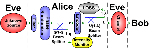
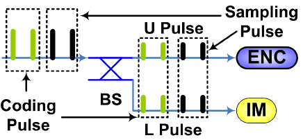
The PNA of our proposed scheme is shown in Figure 2 (b) and the entire scheme is shown in Figure 3. We replaced the 50/50 Optical Switch in Figure 2 (a) by a $q/1-q$ Beam Splitter in Figure 2 (b). In this scheme, each input pulse is passively split into two: One (defined as U pulse) is sent to the encoder and transmitted to Bob, and the other (defined as L pulse) is sent to the intensity monitor. The visualization of U/L pulses is shown in Figure 4.

One may naïvely think that since the beam splitting ratio $q$ is known, one can easily estimate the photon number of the U pulse from the measurement result of photon number of the corresponding L pulse. However, this is not true. Any input pulse, after the phase randomization, is in a number state. Therefore, for a pair of U and L pulses originating from the same input pulse, the total photon number of the two pulses is an unknown constant. This restriction suggests that we should not treat the photon numbers of such two pulses as independent variables, and the random sampling theorem cannot be directly applied.

Figure 4: Visualization of different types of pulses. BS: Beam Splitter. ENC: Encoder. IM: Intensity Monitor. Each input pulse is randomly assigned as either a coding pulse or a sampling pulse. After entering the beam splitter, each pulse is split into a U pulse that enters the encoder, and an L pulse that enters the intensity monitor. As a result, there are four types of pulse: coding U pulse, coding L pulse, sampling U pulse, and sampling L pulse.

To bridge the active scheme (in Figure 2 (a)) and the passive scheme (in Figure 2 (b)), we introduce a virtual setup (in Figure 2 (c)). We call such a virtual set-up a “hybrid” scheme because it has features from both the active and the passive schemes.

We assume that the inefficiency of the intensity monitor can be modeled as an additional loss [28]. In the passive scheme (Figure 2 (b)), assuming that the efficiency of the intensity monitor is $\eta_{\mathrm{IM}}\leq 1$, the probability that an input photon is detected is

$$q^{\prime}=(1-q)\eta_{\mathrm{IM}}.$$ (3)

Therefore, we could model the $q/1-q$ beam splitter and the inefficient intensity monitor in Figure 2 (b) as a $q^{\prime}/1-q^{\prime}$ beam splitter and a perfect intensity monitor as in Figure 2 (c).

The above modification changes the probability that an input photon is sent to Bob. To ensure that an identical attenuation is applied to the coding pulses in both the passive scheme (in Figure 2 (b)) and the hybrid scheme (in Figure 2 (c)), we re-define the internal transmittance in the virtual setup as

$$\lambda^{\prime}=q\lambda/q^{\prime}\leq 1$$ (4)

For a given input photon number distribution, the output photon number distribution is determined by the internal loss [21]. Since the internal losses in the passive scheme and the hybrid scheme are identical, for a given input photon number distribution (which can be unknown), the output photon number distributions of the passive scheme is identical to that of the hybrid scheme. Moreover, the photon number distributions obtained by the intensity monitors are also identical for these two schemes.

Note that this virtual set-up is not actually used in an experiment, but is purely for building the equivalence between the active and the passive schemes.

By putting Equations (3) and (4) together, we have one constraint:

$$\lambda^{\prime}=\frac{q\lambda}{(1-q)\eta_{\mathrm{IM}}}\leq 1.$$ (5)

This constraint is very easy to meet in an actual experiment as $\lambda$ can be lower than $10^{-6}$ in a practical set-up [21], $q/(1-q)\leq 100$ in typical beam splitters, and $\eta_{\mathrm{IM}}$ can be greater than 50% in commercial photo diodes .

The resolution of the intensity monitor is another important imperfection. In a real experiment, the intensity monitor may indicate a certain pulse contains $m^{\prime}$ photons. Here we refer to $m^{\prime}$ as the measured photon number in contrast to the actual photon number $m$. However, due to the noise and the inaccuracy of the intensity monitor, this pulse may not contain exactly $m^{\prime}$ photons. To quantify this imperfection, we introduce a term “the conservative interval” $\varsigma$. We then define $\underline{V}^{\mathrm{L}}$ as the number of L pulses with measured photon number $m^{\prime}\in[(1-\delta)M+\varsigma,(1+\delta)M-\varsigma]$. One can conclude that, with confidence level $\tau_{\mathrm{c}}=1-c(\varsigma)$, the number of untagged L bits $V^{\mathrm{L}}\geq\underline{V}^{\mathrm{L}}$. One can make $c(\varsigma)$ arbitrarily close to 0 by choosing large enough $\varsigma$ . The conservative interval is a statistical property rather than an individual property. That is, for one individual pulse, the probability that $|m-m^{\prime}|>\varsigma$ can be non-negligible.

In the virtual setup, input pulses are treated in the same manner as in the active estimate scheme: Coding pulses are routed to the encoder and then sent to Bob, while the sampling pulses are routed to the perfect intensity monitor to measure their photon numbers. We can use the measurement results of sampling pulses to estimate the number of untagged bits in the coding pulses. Knowing the number of untagged bits, one can easily calculate the upper and lower bounds of the output photon number probabilities [21].

Since the passive scheme and the hybrid scheme share the same source, the output photon number distribution is solely determined by the internal loss. The internal transmittances for the coding bits are the same ($q^{\prime}\lambda^{\prime}=q\lambda$) for both schemes. Therefore, the upper and lower bounds of output photon number probabilities estimated from the hybrid scheme are also valid for those of the passive scheme.

Corollary 1.

Consider $k$ pulses sent from an unknown and untrusted source to Alice, where $k$ is a large positive integer. Alice randomly assigns each input pulse as either a sampling pulse or a coding pulse with equal probabilities. Define variables $V_{\mathrm{s}}^{\mathrm{L}}$ and $V_{\mathrm{c}}^{\mathrm{U}}$ as the number of untagged sampling L pulses and the number of untagged coding U pulses, respectively. Here U pulses are defined as pulses sent to the Encoder in Figure 4, and L pulses are defined as pulses sent to the Intensity Monitor in Figure 4. Alice can conclude that $V_{\mathrm{c}}^{\mathrm{U}}>V_{\mathrm{s}}^{\mathrm{L}}-\epsilon_{1}k$ with confidence level $\tau_{1}\geq 1-e^{-k\epsilon_{1}^{2}/2}$. Here $\epsilon_{1}$ is a small positive real number chosen by Alice and Bob. To calculate the upper and lower bounds of output photon number probabilities, one should use equivalent internal transmittance $\lambda^{\prime}$, which is given in Equation (5), instead of actual internal transmittance $\lambda$.

Proof.

The sampling L pulses are sent to a perfect intensity monitor with a probability $q^{\prime}=q\eta_{\text{IM}}$. If we apply the same transmittance $q^{\prime}$ to the coding U pulses, we can consider that sampling L pulses and the coding U pulses as a group of pulses that go through the same attenuation, and we randomly assign each pulse in the group as either a sampling L pulse or a coding U pulse with equal probabilities. Therefore, one can conclude that $V_{\mathrm{c}}^{\mathrm{U}}>V_{\mathrm{s}}^{\mathrm{L}}-\epsilon_{1}k$ with confidence level $\tau_{1}\geq 1-e^{-k\epsilon_{1}^{2}/2}$ by applying Lemma 1. Since the overall transmittance for the U pulses is $q\lambda$, the internal transmittance for the untagged coding U pulses should be considered as $\lambda^{\prime}=q\lambda/q^{\prime}$. ∎

There is no physical location (eg. between the Beam Splitter and the Encoder in Figure 4) where the U pulses see a transmittance of $q^{\prime}$ in the passive scheme. The output photon number probabilities of the coding U pulses are analyzed in the following manner: The coding U pulses, after propagating through a virtual transmittance $q^{\prime}$, contains $V_{\text{c}}^{\text{U}}$ untagged bits. These coding U pulses then propagate through another virtual transmittance $\lambda^{\prime}$, and we can calculate the output photon number probabilities, which is identical to the output photon number probabilities generated by sending the coding U pulses through the real transmittance $q\lambda=q^{\prime}\lambda^{\prime}$.

Note that, it is not clear to us how to use random sampling theorem to estimate the number of untagged coding “U” pulses from the number of untagged coding “L” pulses. This is due to the correlations between corresponding “L” and “U” pulses. As discussed before, their photon numbers are not independent variables. We are applying a restricted sampling where we draw only one sample from each pair of U and L pulses.

A common imperfection is the inaccuracy of beam splitting ratio $q$. One can calibrate the value of $q$, but only with a finite resolution. In the security analysis, one should pick the most conservative value of $q$ within the calibrated range. That is, the value of $q$ that suggests the lowest key generation rate. Similar strategy should be applied to the inaccuracy of internal transmittance $\lambda$.

4 Efficient Passive Estimate on Untrusted Source

In the above analysis, only half pulses (coding pulses) are used to generate the secure key. Note that we can also use the measurement result of coding “L” pulses to estimate the number of untagged sampling “U” pulses as there is no physical difference between sampling pulses and coding pulses. Note that Alice has the knowledge of the number of untagged coding “L” pulses. We have the following statement:

Corollary 2.

Consider $k$ pulses sent from an unknown and untrusted source to Alice, where $k$ is a large positive integer. Alice randomly assigns each input pulse as either a sampling pulse or a coding pulse with equal probabilities. Define variables $V_{\mathrm{c}}^{\mathrm{L}}$ and $V_{\mathrm{s}}^{\mathrm{U}}$ as the number of untagged coding L pulses and the number of untagged sampling U pulses, respectively. Here U pulses are defined as pulses sent to the Encoder in Figure 4, and L pulses are defined as pulses sent to the Intensity Monitor in Figure 4. Alice can conclude that $V_{\mathrm{s}}^{\mathrm{U}}>V_{\mathrm{c}}^{\mathrm{L}}-\epsilon_{2}k$ with confidence level $\tau_{2}\geq 1-e^{-k\epsilon_{2}^{2}/2}$. Here $\epsilon_{2}$ is a small positive real number chosen by Alice and Bob.

A natural question is: Since Alice has the knowledge about both $V_{\mathrm{s}}^{\mathrm{L}}$ and $V_{\mathrm{c}}^{\mathrm{L}}$, how can she estimate the number of total untagged U pulses, $V^{\mathrm{U}}(=V_{\mathrm{s}}^{\mathrm{U}}+V_{\mathrm{c}}^{\mathrm{U}})$?

Combining all untagged U bits is not entirely trivial. Consider that the untrusted source generates $k$ pulses. Each of them is divided into 2 pulses. Therefore Alice and Bob have $2k$ pulses to analyze. However, these $2k$ pulses are not independent because the beam splitter clearly creates correlations between the corresponding L pulse and U pulse. A naïve application of the random sampling theorem, ignoring the correlation between U pulses and L pulses, may lead to security loophole.

Lemma 2.

Consider $k$ pulses sent from an unknown and untrusted source to Alice. Alice randomly assigns each input pulse as either a sampling pulse or a coding pulse with equal probabilities. Each input pulse is split into a U pulse and an L pulse (see Figure 4 for visualization). The probability that $V^{\mathrm{U}}\leq V_{\mathrm{s}}^{\mathrm{L}}+V_{\mathrm{c}}^{\mathrm{L}}-\epsilon_{1}k-\epsilon_{2}k$ satisfies:

$$P(V^{\mathrm{U}}\leq V_{\mathrm{s}}^{\mathrm{L}}+V_{\mathrm{c}}^{\mathrm{L}}-(\epsilon_{1}+\epsilon_{2})k)\leq\exp(\frac{-k\epsilon_{1}^{2}}{2})+\exp(\frac{-k\epsilon_{2}^{2}}{2}).$$ (6)

Proof.

See D. ∎

In real experiment, it is convenient to count all the untagged L pulses, defined as variable $V^{\mathrm{L}}(=V_{\mathrm{s}}^{\mathrm{L}}+V_{\mathrm{c}}^{\mathrm{L}})$. Can we estimate $V^{\mathrm{U}}$ directly from $V^{\mathrm{L}}$?

Proposition 1.

Consider $k$ pulses sent from an unknown and untrusted source to Alice. Alice randomly assigns each input pulse as either a sampling pulse or a coding pulse with equal probabilities. The probability that $V^{\mathrm{U}}\leq V^{\mathrm{L}}-\epsilon k$ satisfies:

$$P(V^{\mathrm{U}}\leq V^{\mathrm{L}}-\epsilon k)\leq 2\exp(\frac{-k\epsilon^{2}}{4})$$ (7)

That is, Alice can conclude that $V^{\mathrm{U}}>V^{\mathrm{L}}-\epsilon k$ with confidence level

$$\tau>1-2\exp(\frac{-k\epsilon^{2}}{4})$$ (8)

Proof.

This is a natural conclusion from Lemma 2. Note that $V^{\mathrm{L}}=V_{\mathrm{s}}^{\mathrm{L}}+V_{\mathrm{c}}^{\mathrm{L}}$. If Alice chooses $\epsilon_{1}=\epsilon_{2}=\epsilon/2$, Equation (6) reduces to Equation (7). ∎

Once the number of untagged bits that are sent to Bob is estimated, the final key generation rate can be calculated [21].

5 Numerical Simulation

We performed numerical simulation to test the efficiencies of the active and passive estimates. Here, we define the key generation rate as secure key bits per pulse sent by the source, which may be controlled by an eavesdropper. This is different from the definition used in [21], where the key generation rate is defined as secure key bit per pulse sent by Alice. Note that, in the passive scheme, all the pulses sent by the source are sent from Alice to Bob, while in active scheme, only half of the pulses sent by the source are sent from Alice to Bob. Therefore, for the same set-up, we can expect the key generation rate suggested by the passive scheme to be roughly twice as high as that by the active scheme. However, the equivalent input photon number in the passive scheme is lower than that of the active scheme, which introduces a competing factor. The comparison between passive and active estimates is discussed in following sections.

5.1 Simulation Techniques

The simulation technique in this paper is similar to that presented in [21] with a few improvements. Here we briefly reiterate it: First, we simulate the experimental outputs based on the parameters reported by [29], which are shown in Table 1. At this stage, we assume that the source is Poissonian with an average output photon number $M$. For a QKD setup with channel transmittance $\eta(=e^{-\alpha l}$, where $\alpha$ is the fiber loss coefficient, and $l$ is the fiber length between Alice and Bob), Bob’s quantum detection efficiency $\eta_{\text{Bob}}$, detector intrinsic error rate $e_{\text{det}}$ and background rate $Y_{0}$, the gain [30] and the QBER of the signals are expected to be [10]

$$Q_{e} =Y_{0}+1-\exp(-\eta\eta_{\text{Bob}}M\lambda),$$ (9)

$$E_{e} =\frac{e_{0}Y_{0}+e_{\text{det}}[1-\exp(-\eta\eta_{\text{Bob}}M\lambda)]}{Q_{e}},$$

respectively. Here $Q_{e}$ and $E_{e}$ refer to the experimentally measured overall properties rather than the properties of the untagged bits. Second, we calculate the secure key generation rate. The general expression of secure key generation rate per pulse sent by Alice is given by [5, 9]

$$R\geq\frac{1}{2}[-Q_{e}f(E_{e})H_{2}(E_{e})+Q_{1}(1-H_{2}(e_{1}))],$$ (10)

where $f(\geq 1)$ is the bi-directional error correction inefficiency ($f=1$ iff the error correction procedure achieves the Shannon limit), $H_{2}$ is the binary Shannon entropy, $Q_{1}$ is the gain of the single photon state in untagged bits, and $e_{1}$ is the QBER of the single photon state in untagged bits. $Q_{e}$ and $E_{e}$ can be experimentally measured. Here, we use Equations (9) to simulate the experimental outputs.

$Q_{1}$ and $e_{1}$ need to be estimated. Here, we use the method described in B. The key assumption for decoy state QKD with an untrusted source is that $Y_{m,n}$ is identical for different states, and so is $e_{m,n}$ [21]. Here $Y_{m,n}$ is the conditional probability that Bob’s detectors click given that this bit enters Alice’s lab with photon number $m$ and emits from Alice’s lab with photon number $n$, and $e_{m,n}$ is the QBER of bits with $m$ input photons and $n$ output photons.

At the second stage, we do not make any assumption about the source. That is, Alice and Bob have to characterize the source from the experimental output. Note that we need to set the values of $\lambda$ and $\delta$ (recall that all untagged bits have input photon numbers $m\in[(1-\delta)M,(1+\delta)M]$, where $\delta$ is a small positive real number, $M$ is a large positive integer, and both $\delta$ and $M$ are chosen by Alice and Bob). It is preferable to set $\lambda$ and $\delta$ to the values that yield the highest final key generation rate. We optimize the values of $\lambda$ and $\delta$ numerically by exhaustive search. Moreover, in the simulation of decoy state QKD with a finite data size, we also need to optimize the portion of each state.

As a clarification, our security analysis does not require any additional assumptions of the source to analyze experimental outputs.

An important improvement is that the value of $\delta$ is optimized at all distances in the following simulations, while $\delta$ is set to be constant in [21]. This is because for different channel losses, the optimal value of $\delta$ can vary. Moreover, several important practical factors are considered, including the unique characteristic of plug & play structure, intensity monitor imperfections, and finite data size.

Figure 5: Simulation result of GLLP [5] protocol with infinite data size, symmetric beam splitter, perfect intensity monitor, and uni-directional structure. We assume that the source is Poissonian centered at $M=10^{6}$ photons per pulse, and the beam splitting ratio $q=0.5$. Citing experimental parameters from Table 1. We calculated the ratio of the key generation rate with an untrusted source over that with a trusted source. For the passive estimate scheme, the ratios are 98.4%, 98.1%, and 79.8% at 1 km, 20 km, and 40 km, respectively. For the active estimate scheme, the ratios are 49.4%, 49.3%, and 42.8% at 1 km, 20 km, and 40 km, respectively.

For ease of calculation, similar to in [21], we approximate the Poisson distribution as a Gaussian distribution centered at $M$ with variance $\sigma^{2}=M$. This is an excellent approximation because $M$ is very large ($10^{3}$ or larger) in all the simulations presented below.

There are various types of imperfections and errors. We will consider them one by one in the following sections. In Section 5.3, we consider the asymmetry of the beam splitter. In Section 5.4, we consider the source attenuation introduced by the bi-directional scheme. In Section 5.5, we consider the inefficiency and the inaccuracy of the intensity monitor. In Section 5.6, we consider the statistical fluctuation due to a finite data size.

5.2 Infinite Data Size with Perfect Intensity Monitor

In the asymptotic case, Alice sends infinitely many bits to Bob (i.e., $k\rightarrow\infty$). Therefore we can set $\epsilon\rightarrow 0$ while still having $\tau\rightarrow 1$.

We assume that the intensity monitor is efficient and noiseless. Similarly to the case in [21], we set $M=10^{6}$. Moreover, we set $q=0.5$ as 50/50 beam splitter is widely used in many applications.

Table 1: Simulation Parameter from GYS [29].

$\eta_{\mathrm{det}}$	$\alpha$	$Y_{0}$	$e_{\mathrm{det}}$
4.5%	0.21dB/km	$1.7\times 10^{-6}$	3.3%

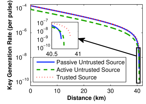
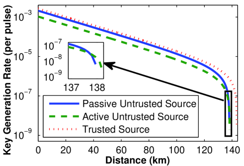
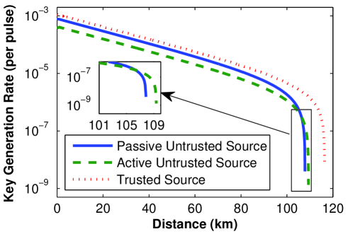
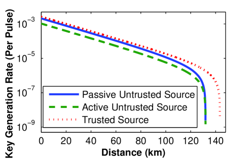
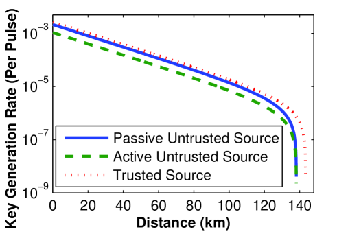
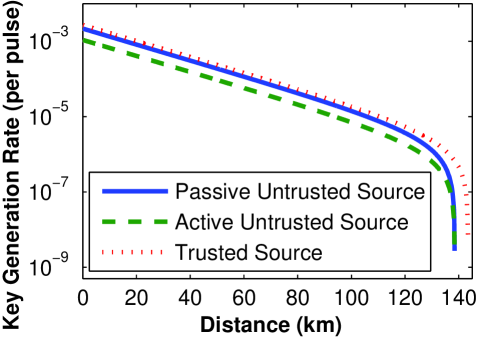
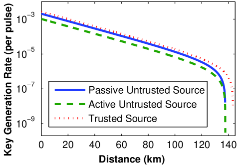
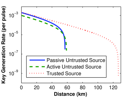
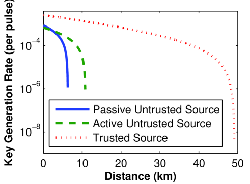
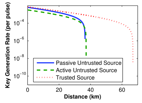
The simulation results of the GLLP protocol [5], Weak+Vacuum decoy state protocol [10], and One-Decoy protocol [10] are shown in Figure 5, Figure 6, and Figure 7, respectively. We can see that the key generation rate of the passive estimate scheme on an untrusted source is very close to that on a trusted source, while the key generation rate of the active estimate scheme is roughly $1/2$ of that of the passive scheme. This is expected because in the active scheme, only half of the pulses generated by the source are sent to Bob, whereas in the passive scheme, all the pulses generated by the source are sent to Bob. Note that, in the asymptotic case, the efficiency of the active estimate scheme can be doubled by sending most pulses (asymptotically all the pulses) to Bob. In this case, there are still infinitely many pulses sent to the Intensity Monitor.

Figure 6: Simulation result of Weak+Vacuum [10] protocol with infinite data size, symmetric beam splitter, perfect intensity monitor, and uni-directional structure. We assume that the source is Poissonian centered at $M=10^{6}$ photons per pulse, and the beam splitting ratio $q=0.5$. Citing experimental parameters from Table 1. We calculated the ratio of the key generation rate with an untrusted source over that with a trusted source. For the passive estimate scheme, the ratios are 77.7%, 77.1%, and 73.8% at 1 km, 50 km, and 100 km, respectively. For the active estimate scheme, the ratios are 39.2%, 39.0%, and 37.4% at 1 km, 50 km, and 100 km, respectively.

For ease of discussion, in passive estimate scheme, we define untagged bits as bits with input photon number $m_{\mathrm{p}}\in[(1-\delta_{\mathrm{p}})M_{\mathrm{p}},(1+\delta_{\mathrm{p}})M_{\mathrm{p}}]$, while in active estimate scheme, we define untagged bits as bits with input photon number $m_{\mathrm{a}}\in[(1-\delta_{\mathrm{a}})M_{\mathrm{a}},(1+\delta_{\mathrm{a}})M_{\mathrm{a}}]$. Here $\delta_{\mathrm{p}}$ and $\delta_{\mathrm{a}}$ are small positive real numbers chosen by Alice and Bob, and $M_{\mathrm{p}}$ and $M_{\mathrm{a}}$ are large positive integers chosen by Alice and Bob. In the passive estimate scheme, we define the maximum possible tagged ratio as $\Delta_{\mathrm{p}}$. In active estimate scheme, we define the maximum possible tagged ratio as $\Delta_{\mathrm{a}}$. Here the tagged ratio is defined as the ratio of the number of tagged bits over the number of all the bits sent to Bob.

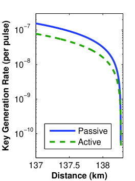
By magnifying the tails at long distances (shown in the insets of Figures 5 – 7), we can see that the active schemes suggest higher key generation rate than the passive schemes do in all three protocols. This behavior is related to the following fact: In the passive estimate scheme, the equivalent input photon number is lower than that of the active estimate scheme. This is because the input photon number is defined as the photons counted by the intensity monitor, and only a portion of an input pulse is sent to the intensity monitor in the passive scheme. Compared to the active scheme, lower input photon number in the passive scheme leads to a larger coefficient of variation of measured input photon number distribution, assuming the source is Poissonian. Therefore, for the same source, if one set $\delta_{\mathrm{p}}=\delta_{\mathrm{a}}$, $\Delta_{\mathrm{p}}$ will be greater than $\Delta_{\mathrm{a}}$ . Increasing the coefficient of variation of the measured input photon number distribution will in general deteriorate the efficiency of the estimate for QKD with untrusted sources. Take two extreme cases for example: If the coefficient of variation is very large, which means the input photon number distribution is almost a uniform distribution, then the estimate efficiency will be very poor because either $\delta$ or $\Delta$ (or both) will be very large. If the coefficient of variation is very small, which means the input photon number distribution is almost a delta-function, then the estimate efficiency will be very good because both $\delta$ and $\Delta$ can be very small.

Figure 7: Simulation result of One-decoy [10] protocol with infinite data size, symmetric beam splitter, perfect intensity monitor, and uni-directional structure. We assume that the source is Poissonian centered at $M=10^{6}$ photons per pulse, and the beam splitting ratio $q=0.5$. Citing experimental parameters from Table 1. We calculated the ratio of the key generation rate with an untrusted source over that with a trusted source. For the passive estimate scheme, the ratios are 71.5%, 68.6%, and 39.5% at 1 km, 50 km, and 100 km, respectively. For the active estimate scheme, the ratios are 38.0%, 36.7%, and 24.4% at 1 km, 50 km, and 100 km, respectively.

The estimate of the gain of untagged bits is very sensitive to the value of $\Delta$, especially when the experimental measured overall gain is small (i.e., when the distance is long, which corresponds to the tails of Figures 5 – 7). The estimate of untagged bits’ gain is discussed in Section III of [21]. Here we briefly recapitulate the main idea: Alice cannot in practice perform a quantum non-demolition measurement on the photon numbers of input pulses. Therefore, Alice and Bob do not know which bits are tagged and which are untagged, though they can estimate the minimum number of untagged bits. Without knowing which bits are untagged, Alice and Bob cannot measure the exact gain $Q$ of untagged bits. Alice and Bob can only experimentally measure the overall gain $Q_{e}$, which contains contributions from both tagged bits and untagged bits.

Alice and Bob can still estimate the upper and lower bounds of $Q$. They can first estimate the maximum tagged ratio $\Delta$. This estimate can be obtained either actively as proposed in [21], or passively as discussed in this paper. Alice and Bob can then estimate the upper and lower bounds of $Q$ as follows [21]:

$$\overline{Q} =\frac{Q_{e}}{1-\Delta-\epsilon},$$ (11)

$$\underline{Q} =\max\left(0,\frac{Q_{e}-\Delta-\epsilon}{1-\Delta-\epsilon}\right);$$

(a) $q=0.5$

(b) $q=0.01$

Figure 8: Simulation results for Weak+Vacuum protocol [10] with different beam splitters for passive estimate. We assume that the data size is infinite, the intensity monitor is perfect, the source is Poissonian centered at $M=10^{6}$ photons per pulse, and the system is in uni-directional structure. Citing experimental parameters from Table 1. The results are focused at the maximum transmission distance to illustrate the improvement of passive estimate by using a biased beam splitter that sends more photons into the intensity monitor. This is equivalent to increasing input photon numbers in passive scheme.

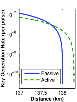
$\underline{Q}$ is very sensitive to $\Delta$ when $Q_{e}$ is small. Therefore, when the distance is long (which corresponds the tails of Figures 5 – 7), $Q_{e}$ becomes very small, and $\underline{Q}$ will then be very sensitive to $\Delta$. Since $\Delta_{\mathrm{p}}>\Delta_{\mathrm{a}}$, the passive estimate becomes less efficient than the active estimate in this case.

On the other hand, in short distances, $Q_{e}$ is significantly greater than $\Delta_{\mathrm{p}}$ and $\Delta_{\mathrm{a}}$, therefore the difference between $\Delta_{\mathrm{p}}$ and $\Delta_{\mathrm{a}}$ makes a negligible contribution to the performance difference between the passive and active estimates. At short distances, it is the following fact that dominates the performance difference between these two schemes: The passive estimate scheme can send Bob twice as many pulses as the active estimate scheme can.

One can increase $\delta$ to decrease $\Delta_{\mathrm{p}}$. That is, if one intends to ensure that $\Delta_{\mathrm{p}}=\Delta_{\mathrm{a}}$, one has to set $\delta_{\mathrm{p}}>\delta_{\mathrm{a}}$. However, increasing $\delta$ also has negative effect on the key generation rate. This is discussed in Section III & IV of [21].

In brief, lower input photon number is the reason why the passive estimate suggests lower key generation rate than the active estimate does around maximum transmission distances in all of the three simulated protocols. This will be confirmed in the simulation presented in Section 5.3 – 5.6.

Figure 9: Simulation result of Weak+Vacuum [10] protocolwith infinite data size, asymmetric beam splitter, perfect intensity monitor, and bi-directional structure. We assume that the source in Bob’s lab is Poissonian centered at $M_{\mathrm{B}}=10^{6}$ photons per pulse, and the beam splitting ratio $q=0.01$. Citing experimental parameters from Table 1. We calculated the ratio of the key generation rate with an untrusted source over that with a trusted source. For passive estimate scheme, the ratios are 78.5%, 75.0%, and 63.0% at 1 km, 50 km, and 100 km, respectively. For active estimate scheme, the ratios are 39.2%, 37.5%, and 31.5% at 1 km, 50 km, and 100 km, respectively. Comparing with Figure 6, we can see that the bi-directional nature of Plug & Play set-up reduced the efficiencies of both active and passive estimates on an untrusted source.

5.3 Biased Beam Splitter

A natural measure to improve the efficiency of the passive estimate is to increase input photon number. Note that in the passive estimate, as discussed in Section 3, input photon numbers are the photon numbers counted by the intensity monitor. Therefore, it can improve the passive estimate’s efficiency to send more photons to the intensity monitor (i.e., setting $q$ smaller).

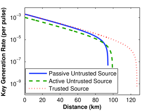
To test this postulate, we performed another simulation to compare the performance of the passive estimate with different values of $q$. Similar to the above subsection, we assume that the intensity monitor is efficient and noiseless, and data size is infinite. Therefore $\epsilon=0$. We set $M=10^{6}$ at the source.

The simulation results are shown in Figure 8. We can clearly see that by setting $q$ to a smaller value (1%), the key generation rate of the passive estimate scheme is improved around the maximum transmission distance.

Intuitively, one can improve the efficiency of the active scheme by sending most pulses to Bob. One can refer to the discussion in C below Equation (31) as a starting point. Detailed discussion of optimizing the efficiency of the active estimate scheme is beyond the scope of the current paper and is subject to further investigation.

Figure 10: Simulation result of Weak+Vacuum [10] protocol with infinite data size, asymmetric beam splitter, perfect intensity monitor, bi-directional structure, and a bright light source. We assume that the source in Bob’s lab is Poissonian centered at $M_{\mathrm{B}}=\mathbf{10^{8}}$ photons per pulse, and the beam splitting ratio $q=0.01$. Citing experimental parameters from Table 1. We calculated the ratio of the key generation rate with an untrusted source over that with a trusted source. For the passive estimate scheme, the ratios are 80.3%, 79.6%, and 75.8% at 1 km, 50 km, and 100 km, respectively. For the active estimate scheme, the ratios are 40.1%, 39.8%, and 37.9% at 1 km, 50 km, and 100 km, respectively. Comparing with Figure 9, we can see that the estimate efficiencies for both the active and passive schemes are improved by using a brighter source.

5.4 Plug & Play Setup

In the Plug & Play QKD scheme, the source is located in Bob’s lab. Bright pulses sent by Bob will suffer the whole channel loss before entering Alice’s lab. Therefore, in the Plug & Play set-up, Alice’s average input photon number is dependent on the channel loss between Alice and Bob. If the average photon number per pulse at the source in Bob’s lab, $M_{\mathrm{B}}$, is constant, the average input photon number per pulse in Alice’s lab, $M$, decreases as the channel loss increases.

Similar to in the above subsection, we assume that the intensity monitor is efficient and noiseless, and data size is infinite. Therefore $\epsilon=0$. We set $M_{\mathrm{B}}=10^{6}$ at the source in Bob’s lab. We set $q=1\%$ to improve the passive estimate efficiency.

We clarify that “distance” in all the simulations of bi-directional QKD set-up refers to a one-way distance between Alice and Bob, not a round-trip distance.

The simulation results of Weak+Vacuum protocol [10] are shown in Figure 9. We can see that the bi-directional nature plug & play structure clearly deteriorates the performance at long distances for which the input photon number on Alice’s side is largely reduced. This affects both the passive and active estimates.

A natural measure to improve the performance of the Plug & Play setup is to use a brighter source. By setting $M_{\mathrm{B}}=10^{8}$ at the source in Bob’s lab, the performances for both passive and active estimates are improved substantially as shown in Figure 10. Note that subnanosecond pulses with $\sim 10^{8}$ photons per pulse can be routinely generated with directly modulated laser diodes.

Figure 11: Simulation result of Weak+Vacuum [10] protocol with infinite data size, asymmetric beam splitter, imperfect intensity monitor, and bi-directional structure. We assume that the intensity monitor efficiency $\eta_{\mathrm{IM}}=0.7$, the intensity monitor noise $\sigma_{\mathrm{IM}}=10^{5}$, the intensity monitor conservative interval $\varsigma=6\times 10^{5}$, the source in Bob’s lab is Poissonian centered at $M_{\mathrm{B}}=10^{8}$ photons per pulse, and the beam splitting ratio $q=0.01$. Citing experimental parameters from Table 1. Comparing with Figure 9, we can see that the imperfections of the intensity monitor substantially reduce the efficiencies of both active and passive estimates.

5.5 Imperfections of the Intensity Monitor

There are two major imperfections of the intensity monitor: inefficiency and noise. These imperfections are discussed in Section 3. The inefficiency can be easily modeled as additional loss in the simulation.

There can be various noise sources, including thermal noise, shot-noise, etc. Here, we consider a simple noise model where a constant Gaussian noise with variance $\sigma_{\mathrm{IM}}^{2}$ is assumed. That is, if $m$ photons enter an efficient but noisy intensity monitor, the probability that the measured photon number is $m^{\prime}$ obeys a Gaussian distribution

$$P_{m}(m^{\prime})=\frac{1}{\sigma_{\mathrm{IM}}\sqrt{2\pi}}\exp[-\frac{(m-m^{\prime})^{2}}{2\sigma_{\mathrm{IM}}^{2}}].$$

The measured photon number distribution $P(m^{\prime})$ has larger variation than the actual photon number distribution $P(m)$ due to the noise of the intensity monitor. More concretely, if the actual photon numbers obeys a Gaussian distribution centered at $M$ with variance $\sigma^{2}$, the measured photon numbers also obeys a Gaussian distribution centered at $M$, but with a variance $\sigma^{2}+\sigma_{\mathrm{IM}}^{2}$.

As in the previous subsections, we assume that the data size is infinite. Therefore $\epsilon=0$. We set $M_{\mathrm{B}}=10^{8}$ at the source in Bob’s lab. Plug & Play set-up is assumed. We set $q=1\%$ to improve the passive estimate efficiency. The imperfections of the intensity monitor are set as follows: the efficiency is set as $\eta_{\mathrm{IM}}=0.7$, and the noise is set as $\sigma_{\mathrm{IM}}=10^{5}$ (see experimental parameters in Section 5.7 and Section 6). For ease of simulation, we assume that the intensity monitor conservative interval is constant over different input photon numbers. We set $\varsigma=6\sigma_{\mathrm{IM}}=6\times 10^{5}$ to ensure a conservative estimate.

Figure 12: Simulation result of Weak+Vacuum [10] protocol with infinite data size, asymmetric beam splitter, imperfect intensity monitor, bi-directional structure, and a very bright source. We assume that the intensity monitor efficiency $\eta_{\mathrm{IM}}=0.7$, the intensity monitor noise $\sigma_{\mathrm{IM}}=10^{5}$, the intensity monitor conservative interval $\varsigma=6\times 10^{5}$, the source in Bob’s lab is Poissonian centered at $M_{\mathrm{B}}=10^{10}$ photons per pulse, and the beam splitting ratio $q=0.01$. Citing experimental parameters from Table 1. Comparing with Figure 11, we can see that using a brighter source can effectively improve the efficiencies of both passive and active estimates. Although it is challenging to build such bright pulsed laser diodes ($10^{10}$ photons per pulse with pulse width less than 1 ns) at telecom wavelengths, one can simply attach a fibre amplifier to the laser diode to generate very bright pulses. Nonetheless, at such a high intensity level, non-linear effects in the fibre, like self phase modulation, may be significant [31].

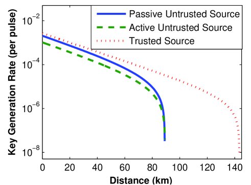
The simulation results for Weak+Vacuum protocol [10] are shown in Figure 11. We can see that the detector noise significantly affects the performance of the Plug & Play QKD system. This is because at long distances, the bi-directional nature of the Plug & Play set-up reduces the input photon number on Alice’s side. Intensity monitor noise and the conservative interval are assumed as constants regardless of the input photon number in our simulation. Therefore they become critical issues when the input photon number is low. As a result, the key generation rate at long distance is substantially reduced.

Figure 13: Simulation result of Weak+Vacuum [10] protocol with infinite data size, asymmetric beam splitter, imperfect intensity monitor, and uni-directional structure. We assume that the intensity monitor efficiency $\eta_{\mathrm{IM}}=0.7$, the intensity monitor noise $\sigma_{\mathrm{IM}}=10^{5}$, the intensity monitor conservative interval $\varsigma=6\times 10^{5}$, the source is Poissonian centered at $M=10^{8}$ photons per pulse, and the beam splitting ratio $q=0.01$. Citing experimental parameters from Table 1. Comparing with Figure 11, we can see that uni-directional structure can effectively improve the efficiencies of both passive and active estimates.

The above postulate is confirmed by the simulations shown in Figure 12 and Figure 13. In Figure 12, we assume that the source in Bob’s lab is extremely bright (sending out $10^{10}$ photons per pulse). We can see clearly that when the input photon number on Alice’s side is high, the key generation rate is only affected slightly by the imperfections of the intensity monitor. Although it is challenging to build such bright pulsed laser diodes ($10^{10}$ photons per pulse with pulse width less than 1 ns) at telecom wavelengths, one can simply attach a fibre amplifier to the laser diode to generate very bright pulses. Nonetheless, at such a high intensity level, non-linear effects in the fibre, like self phase modulation, may be significant [31].

An alternative solution is to use the uni-directional setting, in which the photon number per pulse is constantly high on Alice’s side. From Figure 13 we can see that using the uni-directional setting can also minimize the negative effects introduced by the imperfections of the intensity monitor. Nonetheless, if one adopts the uni-directional QKD scheme, one will lose the unique advantages of bi-directional QKD scheme, like the intrinsic stability against the polarization dispersion and the phase drift. Note that adopting the uni-directional scheme does not mean the coherent state assumption is valid. Indeed, even if Alice possesses the source, the source may not be Poissonian and Alice may not have a full characterization of the source without real-time monitoring.

5.6 Finite Data Size

Real experiments are performed within a limited time, during which the source can only generate a finite number of pulses. To be consistent with previous analysis, we assume that the source generates $k$ pulses in an experiment. Reducing the data size from infinite to finite has two consequences: First, if the confidence level $\tau$ as defined in Equation (8) (for passive estimate) or in Equation (2) (for active estimate) is expected to be close to 1, $\epsilon$ has to be positive. More concretely, for a fixed $k$, if the estimate on the untrusted source is expected to have confidence level no less than $\tau$, one has to pick $\epsilon$ as

$$\epsilon_{\mathrm{p}}=\sqrt{-\frac{4\ln(\frac{1-\tau}{2})}{k}}$$

in the passive estimate scheme, or

$$\epsilon_{\mathrm{a}}=\sqrt{-\frac{2\ln(1-\tau)}{k}}$$

in the active estimate scheme. Second, in decoy state protocols [10], the statistical fluctuations of experimental outputs have to be considered. The technique to analyze the statistical fluctuation in decoy state protocols for numerical simulation is discussed in [10, 12, 14].

Figure 14: Simulation results of the Weak+Vacuum [10] protocol with finite data size, asymmetric beam splitter, imperfect intensity monitor, and bi-directional structure. We assume that the data size is $\mathbf{10^{12}}$, the intensity monitor efficiency $\eta_{\mathrm{IM}}=0.7$, the intensity monitor noise $\sigma_{\mathrm{IM}}=10^{5}$, the intensity monitor conservative interval $\varsigma=6\times 10^{5}$, the source in Bob’s lab is Poissonian centered at $M_{\mathrm{B}}=10^{8}$ photons per pulse, the beam splitting ratio $q=0.01$. Confidence level is set as $\tau\geq 1-10^{-10}$. 6 standard deviations are considered in the statistical fluctuation. Citing experimental parameters from Table 1. Comparing with Figure 11, we can see that finite data size reduces efficiencies of both active and passive estimates.

In the simulation presented in Figure 14, we assume that the data size is $10^{12}$ bits (i.e., the source generates $10^{12}$ pulses in one experiment). This data size is reasonable for the optical layer of the QKD system because because reliable gigahertz QKD implementations have been reported in several recent works [27, 32, 33]. $10^{12}$ bits can be generated within a few minutes in these gigahertz QKD systems. We set the confidence level as $\tau\geq 1-10^{-10}$, which suggests $\epsilon_{\mathrm{a}}=6.79\times 10^{-5}$ and $\epsilon_{\mathrm{p}}=9.74\times 10^{-5}$. We consider 6 standard deviations in the statistical fluctuation analysis of Weak+Vacuum protocol.

As in the previous subsections, we set $M_{\mathrm{B}}=10^{8}$ at the source in Bob’s lab. A Plug & Play set-up is assumed. We set $q=1\%$ to improve the passive estimate efficiency. The imperfections of the intensity monitor are set as follows: the efficiency is set as $\eta_{\mathrm{IM}}=0.7$, and the noise is set constant as $\sigma_{\mathrm{IM}}=10^{5}$. The intensity monitor conservative interval is set constant as $\varsigma=6\sigma_{\mathrm{IM}}=6\times 10^{5}$.

The simulation results for the Weak+Vacuum protocol [10] are shown in Figure 14. We can see that finite data size clearly reduces the efficiencies of both active and passive estimates. The aforementioned two consequences of finite data size contribute to this efficiency reduction: First, $\epsilon$ is non-zero in this finite data size case. Therefore, the estimate of the lower bound of untagged bits’ gain is worse as reflected in Equation (11). Note that $\epsilon$ has the same weight as $\Delta$ in Equation (11). Second, the statistical fluctuation for the Weak+Vacuum protocol becomes important [14]. Moreover, the tightness of bounds suggested in Lemma 1, Lemma 2, and Proposition 1 may also affect the estimate efficiency in finite data size.

Figure 15: Simulation result of Weak+Vacuum [10] protocol with finite data size, asymmetric beam splitter, imperfect intensity monitor, bi-directional structure, and very bright source. We assume that the data size is $10^{12}$, the intensity monitor efficiency $\eta_{\mathrm{IM}}=0.7$, the intensity monitor noise $\sigma_{\mathrm{IM}}=10^{5}$, the intensity monitor conservative interval $\varsigma=6\times 10^{5}$, the source in Bob’s lab is Poissonian centered at $M_{\mathrm{B}}=\mathbf{10^{10}}$ photons per pulse, the beam splitting ratio $q=0.01$. Confidence level is set as $\tau\geq 1-10^{-10}$. 6 standard deviations are considered in the statistical fluctuation. Citing experimental parameters from Table 1. Comparing with Figure 11, we can see that using a very bright source can improve efficiencies of both active and passive estimates.

As we showed in Section 5.5, using a very bright source can improve the efficiencies of both passive and active estimates. Here we again adjust the source intensity in Bob’s lab as $M_{\mathrm{B}}=10^{10}$. The results are shown in Figure 15. We can see that using a very bright source can improve the efficiencies of both passive and active estimates in finite data size case. As we mentioned in Section 5.5, such brightness ($10^{10}$ photons per pulse) is achievable with a pulsed laser diode and a fibre laser amplifier. However, non-linear effects should be carefully considered [31].

In future studies, it would be worthwhile to incorporate the finite key length security analyses [34, 35, 36, 37, 38] in the key generation rate calculation.

5.7 Simulating the Set-up in [28]

Figure 16: Simulation result of Weak+Vacuum [10] protocol based on the experimental parameters in [28]: Data size is $9.05\times 10^{7}$ (this data size is reported in [28]. It is smaller than the data size we assumed in other simulations. If a larger data size was used, we would expect some improvements on the simulation results), the intensity monitor efficiency $\eta_{\mathrm{IM}}=0.8$, the intensity monitor noise $\sigma_{\mathrm{IM}}=3.097\times 10^{5}$, the intensity monitor conservative interval $\varsigma=6\sigma_{\mathrm{IM}}$, the source at Bob’s side is Poissonian centered at $M_{\mathrm{B}}=6.411\times 10^{7}$ photons per pulse, the beam splitting ratio $q=0.05$, and the system is in Plug & Play. Confidence level is set as $\tau\geq 1-10^{-10}$. 6 standard deviations are considered in the statistical fluctuation. Single photon detector efficiency is $4\%$, detector error rate is $1.39\%$, and background rate $Y_{0}=9.38\times 10^{-5}$. Comparing with Figure 14, we can see that higher background rate limits the system performance.

[28] reports so far the only experimental implementation of QKD that considers the untrusted source imperfection. However, as we discussed above, the analysis proposed in [28] is challenging to use, and was not applied to analyze the experimental results reported in the same paper. Our analysis, however, provides a method to understand the experimental results of [28]. Here, we present a numerical simulation of the system used in [28].

We have to characterize the noise and conservative interval of the intensity monitor used in [28]. The experimental results reported in [28] show that the measured input photon number distribution is centered at $M=1.818\times 10^{7}$ with a standard deviation $3.097\times 10^{5}$ on Alice’s side. If we assume the source at Bob’s side as Poissonian, the actual input photon number distribution on Alice’s side will also be Poissonian. The detector noise is then $\sigma_{\mathrm{IM}}=\sqrt{(3.097\times 10^{5})^{2}-1.818\times 10^{7}}=3.097\times 10^{5}$. We set the detector conservative interval as constant $\varsigma=6\sigma_{\mathrm{IM}}$.

Source intensity at Bob’s side $M_{\mathrm{B}}$ can be calculated in the following manner: Since $M=1.818\times 10^{7}$ at a distance $l=25$ km, and beam splitting ratio $q=0.05$, we can conclude that

$$M_{\mathrm{B}}=\frac{M}{\alpha l(1-q)}=6.411\times 10^{7}.$$

Here we assume that the fibre loss coefficient $\alpha=-0.21$ dB/km.

The other parameters are directly cited from [28]: The set-up is in Plug & Play structure. The efficiency of the intensity monitor is $\eta_{\mathrm{IM}}=0.8$. Single photon detector efficiency is $4\%$, detector error rate is $1.39\%$, and background rate $Y_{0}=9.38\times 10^{-5}$. As in previous sections, confidence level is set as $\tau\geq 1-10^{-10}$.

In the experiment reported in [28], the data size is $9.05\times 10^{7}$ (it is smaller than the data size we assumed in other simulations. If a larger data size were used, we would expect some improvements on the simulation results). We ran numerical simulation with 6 standard deviations that are considered in the statistical fluctuation. The simulation results are shown in Figure 16. It is encouraging to see that the simulation yields positive key rates for both passive and active estimates at short distances.

5.8 Summary

From the numerical simulations shown in Figures 5 – 16, we conclude that four important parameters can improve the efficiency of passive estimate on an untrusted source: First, the beam splitting ratio $q$ should be very small, say 1%, to send most input photons to the intensity monitor. Second, the light source should be very bright (say, $10^{10}$ photons per pulse). This is particularly important for Plug & Play structure. Third, the imperfections of the intensity monitor should be small. That is, the intensity monitor should have high efficiency (say, over 70%) and high precision (say, can resolve photon number difference of $6\times 10^{5}$). Fourth, the data size should be large (say, $10^{12}$ bits) to minimize the statistical fluctuation.

In brief, a largely biased beam splitter, a bright source, an efficient and precise intensity monitor, and a large data size are four key conditions that can substantially improve the efficiency of the passive estimate on an untrusted source. The latter three conditions are also applicable in the active estimate scheme.

An important advantage of decoy state protocols is that the key generation rate will only drop linearly as channel transmittance decreases [7, 8, 9, 10, 11, 12, 13, 14], while in many non-decoy protocols, like the GLLP protocol [5], the key generation rate will drop quadratically as channel transmittance decreases. In the simulations shown in Figures 6 – 16, we can see that this important advantage is preserved even if the source is unknown and untrusted.

6 Preliminary Experimental Test

We performed some preliminary experiments to test our analysis. The basic idea is to measure some key parameters of our system, especially the characteristics of the source, with which we can perform numerical simulation to show the expected performance.

The experimental set-up is shown in Figure 17. It is essentially a modified commercial plug & play QKD system. We added a 1/99 beam splitter (1/99 BS in Figure 17), a photodiode (PD in Figure 17), and a high-speed oscilloscope (OSC in Figure 17) on Alice’s side. These three parts comprise Alice’s PNA.

Figure 17: Experimental set-up. Alice and Bob: Commercial plug & play QKD system. PD: photodiode. OSC: high-speed oscilloscope. 1/99 BS: 1/99 beam splitter. FM: faraday mirror. PM_x: phase modulators. PBS: polarizing beam splitter. BS: beam splitter. SPD_x: single photon detector. C: circulator.

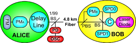
When Bob sends strong laser pulses to Alice, the photodiode (PD in Figure 17) will convert input photons into photoelectrons, which are then recorded by the oscilloscope (OSC in Figure 17). In the recorded waveform, we calculated the area below each pulse. This area is proportional to the number of input photons. The conversion coefficient between the area and photon number is calibrated by measuring the average input laser power on Alice’s side with a slow optical power meter.

In our experiment, 299 700 pulses are generated by the laser diode at Bob’s side (Laser Diode in Figure 17) at a repetition rate of 5 MHz with 1 ns pulse width. They are all split into U pulses and L pulses (see Figure 4) by the 1/99 beam splitter (1/99 BS in Figure 17). The L pulses are measured by a photodiode (PD in Figure 17). The measurement results are acquired and recorded by an oscilloscope (OSC in Figure 17).

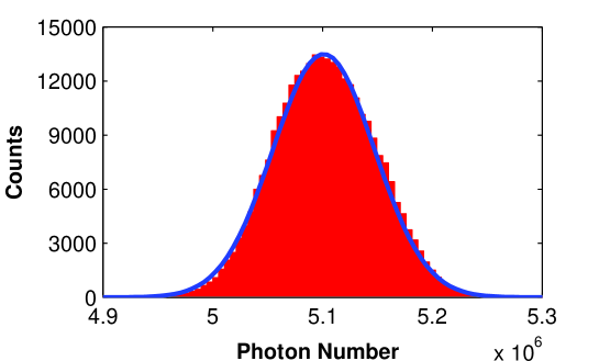
The experimental results of the photon number statistics are plotted in Figure 18. The measured photon number distribution is centered at $M=5.101\times 10^{6}$ photons per pulse, with standard deviation $6.557\times 10^{4}$ on Alice’s side. We can see that the actual photon number distribution fits a Gaussian distribution (shown as the blue line) well. Other experimental results are shown in Table 2.

Table 2: Parameters measured from our preliminary experiment described in Section 6.

$\alpha$	$\eta_{\mathrm{det}}$	$e_{\mathrm{det}}$	$Y_{0}$
-0.21 dB/km	4.89%	0.21%	$8.4\times 10^{-5}$

The intensity monitor noise is calculated in a similar manner to that in Section 5.7: Assuming the source is Poissonian at Bob’s side, which means the actual input photon number on Alice’s side is also Poissonian, the noise is then given by $\sigma_{\mathrm{IM}}=\sqrt{(6.557\times 10^{4})^{2}-5.101\times 10^{6}}=6.553\times 10^{4}.$ As in Section 5.7, we set the detector conservative interval as a constant $\varsigma=6\sigma_{\mathrm{IM}}$.

Source intensity at Bob’s side $M_{\mathrm{B}}$ can be calculated in the following matter (which is similar to the one we used in Section 5.7): Since $M=5.101\times 10^{6}$ at a distance $l=4.8$ km, and beam splitting ratio $q=0.01$, we can conclude that

$$M_{\mathrm{B}}=\frac{M}{\alpha l(1-q)}=6.500\times 10^{6}.$$

Here we know that the fibre loss coefficient $\alpha=-0.21$ dB/km.

Figure 18: Experimentally measured photon number statistics for 299 700 pulses. The distribution centered at $5.101\times 10^{6}$ photons per pulse, with standard deviation $6.557\times 10^{4}$. Blue line shows a Gaussian fit of the actual distribution.

The simulation result is shown in Figure 19, in which the data size is set as $10^{12}$ . We can see that it is possible to achieve positive key rate at moderate distances using the security analysis presented in this paper.

7 Conclusion

In this paper, we present the first passive security analysis for QKD with an untrusted source, with a complete security proof. Our proposal is compatible with inefficient and noisy intensity monitors, which is not considered in [21] or in [28]. Our analysis is also compatible with a finite data size, which is not considered in [28]. Comparing to the active estimate scheme proposed in [21], the passive scheme proposed in this paper significantly reduces the challenges to implement the “Plug & Play” QKD with unconditional security. Our proposal can be applied to practical QKD set-ups with untrusted sources, especially the plug & play QKD set-ups, to guarantee the security.

Figure 19: Simulation result of Weak+Vacuum [10] protocol based on experimental parameters from our QKD system. We assume that the data size is $10^{12}$ bits, the intensity monitor efficiency $\eta_{\mathrm{IM}}=0.7$, the intensity monitor noise $\sigma_{\mathrm{IM}}=6.553\times 10^{4}$, the intensity monitor conservative interval $\varsigma=6\sigma_{\mathrm{IM}}$, the source at Bob’s lab is Poissonian centered at $M_{\mathrm{B}}=6.500\times 10^{6}$ photons per pulse, the beam splitting ratio $q=0.01$, and the system is in the Plug & Play structure. Confidence level is set as $\tau\geq 1-10^{-10}$. 6 standard deviations are considered in the statistical fluctuation. Experimental parameters are listed in Table 2.

We point out four important conditions that can improve the efficiency of the passive estimate scheme proposed in this paper: First, the beam splitter in PNA should be largely biased to send most photons to the intensity monitor. Second, the light source should be bright. Third, the intensity monitor should have high efficiency and precision. Fourth, the data size should be large to minimize the statistical fluctuation. These four conditions are confirmed in extensive numerical simulations.

In the simulations shown in Figures 11 – 16 and Figure 19, we made an additional assumption that the intensity monitor has a constant Gaussian noise. This assumption is not required by our security analysis. It will be interesting to experimentally verify this model in future.

The numerical simulations show that if the above conditions are met, the efficiency of the passive untrusted source estimate is close to that of the trusted source estimate, and is roughly twice as high as the efficiency of the active untrusted source estimate. Nonetheless, the efficiency of active estimate scheme proposed in [21] may be improved to the level that is similar to the efficiency of passive estimation. This is briefly discussed below Equation (30). The security of the improved active estimate scheme is beyond the scope of the current paper, and is subject to further investigation.

Numerical simulations in Figures 6 – 16 and Figure 19 show that the key generation rate drops linearly as the channel transmittance decreases. This is an important advantage of decoy state protocols over many other QKD protocols, and is preserved in our untrusted source analysis.

Our preliminary experimental test highlights the feasibility of our proposed passive estimate scheme. Indeed, our scheme can be easily implemented by making very simple modifications (by adding a few commercial modules) to a commercial Plug & Play QKD system.

A remaining practical question in our proposal is: How to calibrate the noise and the conservative interval of the intensity monitor? Note that these two parameters may not be constant at different intensity levels. Moreover, the noise may not be Gaussian. It is not straightforward to define the conservative interval and its confidence.

Appendix A The Phase Randomization Assumption

In this section, we will show that for the state that is accessible to Eve, Alice’s phase randomization is equivalent to performing a QND measurement on the photon number of the input pulses.

Proof.

Before the phase randomization, the state that is shared by Alice, Bob, and Eve is

$$\mbox{$|\psi\rangle$}_{\text{ABE}}=\sum_{m,n}b_{m,n}\mbox{$|E_{n}\rangle$}\mbox{$|m\rangle$}.$$ (12)

After the phase randomization, a random phase is applied to each pulse, and this phase is inaccessible to Eve. The state becomes

$$\mbox{$|\psi\rangle$}_{\text{ABE}}^{\text{pr}}=\sum_{m,n}b_{m,n}\mbox{$|E_{n}\rangle$}\mbox{$|m\rangle$}e^{im\theta}.$$ (13)

Its density matrix is

$$\rho_{\text{ABE}}^{\text{pr}}=\sum_{m,n,m^{\prime},n^{\prime}}b_{m,n}b^{*}_{m^{\prime},n^{\prime}}\mbox{$|E_{n}\rangle$}\mbox{$\langle E_{n^{\prime}}|$}\otimes\mbox{$|m\rangle$}\mbox{$\langle m^{\prime}|$}e^{i(m-m^{\prime})\theta}.$$ (14)

Since $\theta$ is not known to Eve or Bob, the state that is accessible to Bob and Eve is

$$\rho_{\text{BE}}^{\text{pr}} =\frac{1}{2\pi}\sum_{m,n,m^{\prime},n^{\prime}}b_{m,n}b^{*}_{m^{\prime},n^{\prime}}\mbox{$|E_{n}\rangle$}\mbox{$\langle E_{n^{\prime}}|$}\otimes\mbox{$|m\rangle$}\mbox{$\langle m^{\prime}|$}\int_{0}^{2\pi}e^{i(m-m^{\prime})\theta}\text{d}\theta$$ (15)

$$=\sum_{m,n,n^{\prime}}b_{m,n}b^{*}_{m,n^{\prime}}\mbox{$|E_{n}\rangle$}\mbox{$\langle E_{n^{\prime}}|$}\otimes\mbox{$|m\rangle$}\mbox{$\langle m|$}.$$

Instead of considering the phase randomization, now let us analyze the impact of a photon number measurement on the state given in Equation (12). Before Alice’s measurement, the density matrix is given by

$$\rho_{\text{ABE}}=\sum_{m,n,m^{\prime},n^{\prime}}b_{m,n}b^{*}_{m^{\prime},n^{\prime}}\mbox{$|E_{n}\rangle$}\mbox{$\langle E_{n^{\prime}}|$}\otimes\mbox{$|m\rangle$}\mbox{$\langle m^{\prime}|$}.$$ (16)

After the QND measurement of the photon number, Alice knows the photon number. However, Eve and Bob do not know Alice’s measurement result. Therefore, the state that is accessible to Bob and Eve is given by

$$\rho_{\text{BE}}^{\text{QND}} =\sum_{m^{\prime\prime}}\mbox{$|m^{\prime\prime}\rangle$}\mbox{$\langle m^{\prime\prime}|$}\rho_{\text{ABE}}\mbox{$|m^{\prime\prime}\rangle$}\mbox{$\langle m^{\prime\prime}|$}$$ (17)

$$=\sum_{m,n,n^{\prime}}b_{m,n}b^{*}_{m,n^{\prime}}\mbox{$|E_{n}\rangle$}\mbox{$\langle E_{n^{\prime}}|$}\otimes\mbox{$|m\rangle$}\mbox{$\langle m|$}$$

$$=\rho_{\text{BE}}^{\text{pr}}.$$

∎

From the above equation, we conclude that the two different processes—i) phase randomization by Alice and ii) a photon-number non-demolition measurement—actually give exactly the same density matrix for the Eve-Bob system. Therefore, phase randomization is mathematically equivalent to a photon-number non-demolition measurement. For this reason, we can consider the output state by Alice as a classical mixture of Fock states.

Appendix B Security Analysis for Untagged Bits

In this section, for the convenience of the readers, we recapitulate the security analysis that is presented in [21].

Assume that $k$ pulses are sent from Alice to Bob. Alice and Bob do not know which bits are untagged. However, either from the active estimate presented in [21] or the passive estimate presented in the current paper, they know that at least $(1-\Delta-\epsilon)k$ pulses are untagged with high confidence.

Alice and Bob can measure the overall gain $Q_{e}$ and the overall QBER $E_{e}$. They do not know the gain $Q$ and the QBER $E$ for the untagged bits because they do not know which bits are untagged. Nonetheless, they can then estimate the upper bounds and the lower bounds of them. The upper bound and the lower bound of $Q$ are [21]

$$\overline{Q} =\frac{Q_{e}}{1-\Delta-\epsilon},$$ (18)

$$\underline{Q} =\max(0,\frac{Q_{e}-\Delta-\epsilon}{1-\Delta-\epsilon}).$$

The upper bound and lower bound of $E\cdot Q$ can be estimated as [21]

$$\overline{E\cdot Q} =\frac{Q_{e}E_{e}}{1-\Delta-\epsilon},$$ (19)

$$\underline{E\cdot Q} =\max(0,\frac{Q_{e}E_{e}-\Delta-\epsilon}{1-\Delta-\epsilon}).$$

For untagged bits (i.e., $m\in[(1-\delta)M,(1+\delta)M]$), we can show that the upper bound and the lower bound of the probability that the output photon number from Alice is $n$ are [21]:

$$\overline{P_{n}} =\left\{\begin{array}[]{ll}(1-\lambda)^{(1-\delta)M},&\hbox{if $n=0$;}\\ {(1+\delta)M\choose n}\lambda^{n}(1-\lambda)^{(1+\delta)M-n},&\hbox{if $1\leq n\leq(1+\delta)M$;}\\ 0,&\hbox{if $n>(1+\delta)M$;}\end{array}\right.$$ (20)

$$\underline{P_{n}} =\left\{\begin{array}[]{ll}(1-\lambda)^{(1+\delta)M},&\hbox{if $n=0$;}\\ {(1-\delta)M\choose n}\lambda^{n}(1-\lambda)^{(1-\delta)M-n},&\hbox{if $1\leq n\leq(1-\delta)M$;}\\ 0,&\hbox{if $n>(1-\delta)M$;}\end{array}\right.$$

under Condition 1:

$$(1+\delta)M\lambda<1.$$ (21)

The key rate calculation depends on the QKD protocol that is implemented. For the GLLP [5] protocol with an untrusted source, the key generation rate is given by [21]:

$$R\geq\frac{1}{2}\{-Q_{e}f(E_{e})H_{2}(E_{e})+(\underline{Q}+\underline{P_{0}}+\overline{P_{1}}-1)[1-H_{2}(\frac{Q_{e}E_{e}}{\underline{Q}+\underline{P_{0}}+\overline{P_{1}}-1})]\},$$ (22)

where $Q_{e}$ and $E_{e}$ are measured experimentally, $\underline{Q}$ can be calculated from Equation (18), and $\underline{P_{0}}$ and $\overline{P_{1}}$ can be calculated from Equation (20).

For decoy state protocols [7, 8, 9, 10, 11, 12, 13, 14], the key generation rate (with an untrusted source) is given by [21]:

$$R\geq\frac{1}{2}\{-Q_{e}^{S}f(E_{e}^{S})H_{2}(E_{e}^{S})+(1-\Delta-\epsilon)\underline{Q_{1}^{S}}[1-H_{2}(\overline{e_{1}^{S}})]\},$$ (23)

where $Q_{e}^{S}$ and $E_{e}^{S}$ are the overall gain and the over QBER of the signal states, respectively, and can be measured experimentally. $\underline{Q_{1}^{S}}$ and $\overline{e_{1}^{S}}$ depend on the specific decoy state protocol that is implemented.

For weak+vacuum protocol [10, 11, 14], the lower bound of $Q_{1}^{S}$ for untagged bits is given by [21]:

$$\underline{Q_{1}^{S}}=\underline{P_{1}^{S}}\frac{\underline{Q^{D}}\underline{P_{2}^{S}}-\overline{Q^{S}}\overline{P_{2}^{D}}+(\underline{P_{0}^{S}}\overline{P_{2}^{D}}-\overline{P_{0}^{D}}\underline{P_{2}^{S}})\overline{Q^{V}}-\frac{2\delta M(1-\lambda_{D})^{2\delta M-1}\underline{P_{2}^{S}}}{[(1-\delta)M+1]!}}{\overline{P_{1}^{D}}\underline{P_{2}^{S}}-\underline{P_{1}^{S}}\overline{P_{2}^{D}}}$$ (24)

under Condition 2:

$$\frac{\lambda_{S}}{\lambda_{D}}>\frac{(1+\delta)M-2}{(1-\delta)M-2}\left[\frac{(1+\delta)M-2}{2\delta M}\right]^{\frac{2\delta M}{(1-\delta)M-2}}\left[\frac{(1+\delta)M-2}{(1-\delta)M-2}\cdot\frac{e^{2}}{2\delta M}\right]^{\frac{1}{2[(1-\delta)M-2]}}.$$ (25)

Here $Q^{S}$, $Q^{D}$ and $Q^{V}$ are the gains of untagged bits of the signal state, the decoy state, and the vacuum state, respectively. Their bounds can be estimated from Equations (18). The bounds of the probabilities can be estimated from Equations (20). $\lambda_{S}$ and $\lambda_{D}$ are Alice’s internal transmittances for signal and decoy states, respectively. The upper bound of $e_{1}^{S}$ for untagged bits is given by [21]:

$$e_{1}^{S}\leq\overline{e_{1}^{S}}=\frac{\overline{E^{S}Q^{S}}-\underline{P_{0}^{S}}\underline{E^{V}Q^{V}}}{\underline{Q_{1}^{S}}},$$ (26)

in which $E^{S}$ and $E^{V}$ are the QBERs of untagged bits of the signal and the vacuum states, respectively. $\overline{E^{S}Q^{S}}$ and $\underline{E^{V}Q^{V}}$ can be estimated from Equations (19). $\underline{P_{0}^{S}}$ can be estimated by Equations (20). $\underline{Q_{1}^{S}}$ is given by Equation (24).

For one-decoy protocol [10, 13], a lower bound of $Q_{1}^{S}$ and an upper bound of $e_{1}^{S}$ for untagged bits are given by

$$\underline{Q_{1}^{S}} =\underline{P_{1}^{S}}\frac{\underline{Q^{D}}\underline{P_{2}^{S}}-\overline{Q^{S}}\overline{P_{2}^{D}}+(\underline{P_{0}^{S}}\overline{P_{2}^{D}}-\overline{P_{0}^{D}}\underline{P_{2}^{S}})\frac{\overline{E^{S}Q^{S}}}{\underline{P_{0}^{S}}E^{V}}-\frac{2\delta M(1-\lambda_{D})^{2\delta M-1}\underline{P_{2}^{S}}}{[(1-\delta)M+1]!}}{\overline{P_{1}^{D}}\underline{P_{2}^{S}}-\underline{P_{1}^{S}}\overline{P_{2}^{D}}},$$ (27)

$$\overline{e_{1}^{S}} =\frac{\overline{E^{S}\cdot Q^{S}}}{\underline{Q_{1}^{S}}},$$

respectively, under Condition 2 in the asymptotic case. Here $Q^{S}$ and $Q^{D}$ are the gains of untagged bits of the signal state and the decoy state, respectively. Their bounds can be estimated from Equations (18). $E^{S}$ is the QBER of untagged bits of the signal state. $\overline{E^{S}\cdot Q^{S}}$ can be estimated from Equations (19). $E^{V}=0.5$ in the asymptotic case. The bounds of the probabilities can be estimated from Equations (20).

Appendix C Confidence Level in Active Estimate

Among all the $V$ untagged bits, each bit has probability 1/2 to be assigned as an untagged coding bit. Therefore, the probability that $V_{\mathrm{c}}=v_{\mathrm{c}}$ obeys a binomial distribution. Cumulative probability is given by [39]

$$P(V_{\mathrm{c}}\leq\frac{V-\epsilon k}{2}|V=v)\leq\exp(-\frac{\epsilon^{2}k^{2}}{2v})$$

For any $v\in[0,k]$, $k/v\geq 1$. Therefore, we have

$$P(V_{\mathrm{c}}\leq\frac{V-\epsilon k}{2}|V\in[0,k])\leq\exp(-\frac{k\epsilon^{2}}{2}).$$

In the experiment described by Lemma 1, $V\in[0,k]$ is always true. Therefore, the above inequality reduces to

$$P(V_{\mathrm{c}}\leq\frac{V-\epsilon k}{2})\leq\exp(-\frac{k\epsilon^{2}}{2}).$$ (28)

By definition, we have

$$V=V_{\mathrm{c}}+V_{\mathrm{s}}.$$ (29)

Substituting Equation (29) into Equation (28), we have

$$P(V_{\mathrm{c}}\leq V_{\mathrm{s}}-\epsilon k)\leq\exp(-\frac{k\epsilon^{2}}{2}).\qed$$ (30)

The above proof can be easily generalized to the case where for each bit sent from the untrusted source to Alice, Alice randomly assigns it as either a coding bit with probability $\gamma$, or a sampling bit with probability $1-\gamma$. Here $\gamma\in(0,1)$ is chosen by Alice. It is then straightforward to show that

$$P[V_{\mathrm{c}}\leq\frac{\gamma}{1-\gamma}(V_{\mathrm{s}}-\epsilon k)]\leq\exp(-2k\epsilon^{2}\gamma^{2}).$$ (31)

When $\gamma=1/2$, Equation (31) reduces to Equation (30).

Appendix D Confidence Level in Cross Estimate

From Corollary 1 and Corollary 2, we know that

$$P(V_{\mathrm{c}}^{\mathrm{U}} \leq V_{\mathrm{s}}^{\mathrm{L}}-\epsilon_{1}k)\leq\exp(\frac{-k\epsilon_{1}^{2}}{2})$$ (32)

$$P(V_{\mathrm{s}}^{\mathrm{U}} \leq V_{\mathrm{c}}^{\mathrm{L}}-\epsilon_{2}k)\leq\exp(\frac{-k\epsilon_{2}^{2}}{2}).$$

Therefore, we have

$$P(V^{\mathrm{U}}\leq V_{\mathrm{s}}^{\mathrm{L}}+V_{\mathrm{c}}^{\mathrm{L}}-(\epsilon_{1}+\epsilon_{2})k)$$ (33)

$$= P(V_{\mathrm{c}}^{\mathrm{U}}+V_{\mathrm{s}}^{\mathrm{U}}\leq V_{\mathrm{s}}^{\mathrm{L}}+V_{\mathrm{c}}^{\mathrm{L}}-(\epsilon_{1}+\epsilon_{2})k)$$

$$\leq P[(V_{\mathrm{c}}^{\mathrm{U}}\leq V_{\mathrm{s}}^{\mathrm{L}}-\epsilon_{1}k)$$

$$\text{ or }(V_{\mathrm{s}}^{\mathrm{U}}\leq V_{\mathrm{c}}^{\mathrm{L}}-\epsilon_{2}k)]$$

$$\leq P(V_{\mathrm{c}}^{\mathrm{U}}\leq V_{\mathrm{s}}^{\mathrm{L}}-\epsilon_{1}k)$$

$$+P(V_{\mathrm{c}}^{\mathrm{U}}\leq V_{\mathrm{s}}^{\mathrm{L}}-\epsilon_{2}k)$$

$$= \exp(\frac{-k\epsilon_{1}^{2}}{2})+\exp(\frac{-k\epsilon_{2}^{2}}{2}).$$

In the above derivation, we made use of the fact that $[(V_{\mathrm{c}}^{\mathrm{U}}\leq V_{\mathrm{s}}^{\mathrm{L}}-\epsilon_{1}k)\text{ or }(V_{\mathrm{s}}^{\mathrm{U}}\leq V_{\mathrm{c}}^{\mathrm{L}}-\epsilon_{2}k)]$ is always true if $[V_{\mathrm{c}}^{\mathrm{U}}+V_{\mathrm{s}}^{\mathrm{U}}\leq V_{\mathrm{s}}^{\mathrm{L}}+V_{\mathrm{c}}^{\mathrm{L}}-(\epsilon_{1}+\epsilon_{2})k]$ is true.

References

- [1] C. H. Bennett and G. Brassard, “Quantum Cryptography: Public Key Distribution and Coin Tossing,” in Proceedings of IEEE International Conference on Computers, Systems, and Signal Processing pp. 175 – 179 (1984).
- [2] A. K. Ekert, “Quantum cryptography based on Bell’s theorem,” Phys. Rev. Lett. 67, 661 (1991).
- [3] H.-K. Lo and Y. Zhao, “Quantum Cryptography,” in Encyclopedia of Complexity and System Science (Springer, New York, 2009), Vol. 8, pp. 7265–7289, arXiv:0803.2507.
- [4] D. Mayers, J. of ACM 48, 351 (2001); H.-K. Lo and H. F. Chau, Science 283, 2050 (1999); P. Shor and J. Preskill, Phys. Rev. Lett. 85, 441 (2000).
- [5] D. Gottesman, H.-K. Lo, N. Lütkenhaus, and J. Preskill, “Security of quantum key distribution with imperfect devices,” Quant. Info. Compu. 4, 325 (2004).
- [6] H. Inamori, N. Lütkenhaus, and D. Mayers, “Unconditional Security of Practical Quantum Key Distribution,” European Physical Journal D 41, 599 (2007).
- [7] W. Y. Hwang, “Quantum Key Distribution with High Loss: Toward Global Secure Communication,” Phys. Rev. Lett. 91, 057 901 (2003).
- [8] H.-K. Lo, “Quantum Key Distribution with Vacua or Dim Pulses as Decoy States,” in Proceedings of IEEE International Symposium on Information Theory p. 137 (2004).
- [9] H.-K. Lo, X. Ma, and K. Chen, “Decoy State Quantum Key Distribution,” Phys. Rev. Lett. 94, 230 504 (2005).
- [10] X. Ma, B. Qi, Y. Zhao, and H.-K. Lo, “Practical Decoy State for Quantum Key Distribution,” Phys. Rev. A 72, 012 326 (2005).
- [11] X.-B. Wang, “Beating the Photon-Number-Splitting Attack in Practical Quantum Cryptography,” Phys. Rev. Lett. 94, 230 503 (2005).
- [12] X.-B. Wang, “Decoy-state protocol for quantum cryptography with four different intensities of coherent light,” Phys. Rev. A 72, 012 322 (2005).
- [13] Y. Zhao, B. Qi, X. Ma, H.-K. Lo, and L. Qian, “Experimental Quantum Key Distribution with Decoy States,” Phys. Rev. Lett. 96, 070 502 (2006).
- [14] Y. Zhao, B. Qi, X. Ma, H.-K. Lo, and L. Qian, “Simulation and Implementation of Decoy State Quantum Key Distribution over 60km Telecom Fiber,” in Proceedings of IEEE International Symposium of Information Theory pp. 2094–2098 (2006).
- [15] A. Muller, T. Herzog, B. Hutter, W. Tittel, H. Zbinden, and N. Gisin, “‘Plug & play’ systems for quantum crytography,” Appl. Phys. Lett. 70, 793 (1997).
- [16] D. Stucki, N. Gisin, O. Guinnard, G. Ribordy, and H. Zbinden, “Quantum key distribution over 67 km with a plug&play system,” New J. of Phys. 4, 41 (2002).
- [17] www.idquantique.com.
- [18] www.magiqtech.com.
- [19] G. Pólya, “Über den zentralen Grenzwertsatz der Wahrscheinlichkeitsrechnung und das Momentenproblem (in German),” Mathematische Zeitschrift 8, 171 (1920).
- [20] N. Gisin, S. Fasel, B. Kraus, H. Zbinden, and G. Ribordy, “Trojan horse attacks on quantum key distribution systems,” Phys. Rev. A 73, 022 320 (2006).
- [21] Y. Zhao, B. Qi, and H.-K. Lo, “Quantum Key Distribution with an Unknown and Untrusted Source,” Phys. Rev. A 77, 052 327 (2008).
- [22] P. Villoresi, T. Jennewein, F. Tamburini, M. Aspelmeyer, C. Bonato, R. Ursin, C. Pernechele, V. Luceri, G. Bianco, A. Zeilinger, and C. Barbieri, “Experimental verification of the feasibility of a quantum channel between Space and Earth,” New J. of Phys. 10, 033 038 (2008).
- [23] X.-B. Wang, C.-Z. Peng, and J.-W. Pan, “Simple protocol for secure decoy-state quantum key distribution with a loosely controlled source,” Appl. Phys. Lett. 90, 031 110 (2007).
- [24] X.-B. Wang, C.-Z. Peng, J. Zhang, and J.-W. Pan, “Security of decoy-state quantum key distribution with inexactly controlled source,” quant-ph/0612121v3 (2008).
- [25] X.-B. Wang, C.-Z. Peng, J. Zhang, and J.-W. Pan, “General theory of decoy-state quantum cryptography with source errors,” Phys. Rev. A 77, 043 311 (2008).
- [26] X.-B. Wang, L. Yang, C.-Z. Peng, and J.-W. Pan, “Decoy-state quantum key distribution with both source errors and statistical fluctuations,” New J. of Phys. 11, 075 006 (2009).
- [27] H. Takesue, S. W. Nam, Q. Zhang, R. H. Hadfield, T. Honjo, K. Tamaki, and Y. Yamamoto, “Quantum key distribution over a 40-dB channel loss using superconducting single-photon detectors,” Nature Photonics 1, 343 (2007).
- [28] X. Peng, H. Jiang, B. Xu, X. Ma, and H. Guo, “Experimental quantum key distribution with an untrusted source,” Opt. Lett. 33, 2077 (2008).
- [29] C. Gobby, Z. L. Yuan, and A. J. Shields, “Quantum key distribution over 122 km of standard telecom fiber,” Appl. Phys. Lett. 84, 3762 (2004).
- [30] The gain is defined to be the ratio of the number of receiver Bob’s detection events to the number of signals emitted by sender Alice in the cases where Alice and Bob use the same basis. It depends mainly on the intensity of signal, channel transmittance, and Bob’s quantum efficiency.
- [31] See, like, Gerd Keiser, Optical Fiber Communications, 3rd edition, Chapter 12.5 (McGraw-Hill, 2000).
- [32] Q. Zhang, H. Takesue, T. Honjo, K. Wen, T. Hirohata, M. Suyama, Y. Takiguchi, H. Kamada, Y. Tokura, O. Tadanaga, Y. Nishida, M. Asobe, and Y. Yamamoto, “Megabits secure key rate quantum key distribution,” New J. of Phys. 11, 045 010 (2009).
- [33] A. R. Dixon, Z. L. Yuan, J. F. Dynes, A. W. Sharpe, and A. J. Shields, “Gigahertz decoy quantum key distribution with 1 Mbit/s secure key rate,” Opt. Express 16, 18 790 (2008).
- [34] M. Hayashi, “Practical evaluation of security for quantum key distribution,” Phys. Rev. A 74, 022 306 (2006).
- [35] M. Hayashi, “Upper bounds of eavesdropper’s performances in finite-length code with decoy method,” Phys. Rev. A 76, 012 329 (2007).
- [36] J. Hasegawa, M. Hayashi, T. Hiroshima, and A. Tomita, “Security analysis of decoy state quantum key distribution incorporating finite statistics,” arXiv:0707.3541 (2007).
- [37] V. Scarani and R. Renner, “Quantum Cryptography with Finite Resources: Unconditional Security Bound for Discrete-Variable Protocols with One-Way Postprocessing,” Phys. Rev. Lett. 100, 200 501 (2008).
- [38] X. Ma, C.-H. F. Fung, J.-C. Boileau, and H. F. Chau, “Practical post-processing for quantum-key-distribution experiments,” arXiv:0904.1994 (2009).
- [39] W. Hoeffding, “Probability inequalities for sums of bounded random variables,” J. Am. Stat. Asso. 58, 13 (1963).